Real-Time, Inexpensive, and Portable Measurement of Water Surface Velocity through Smartphone

Abstract

The purpose of this research is to propose a real-time, inexpensive, and portable method for measuring water surface velocities, in which a particle tracking velocimetry (PTV) system is developed by using a smartphone device. The system uses the mobile camera to capture the tracer floating on the river surface, whose movement is expected to represent the velocity of the water surface. The recorded tracer images are identified from the background by using the normalized RGB color model. The magnification ratio, which transforms the distance in pixel to the real distance, is estimated by using the pre-specified mobile height from the water surface, or the characteristic length of the tracer. The proposed system is built based on the iPhone 6s device. The system is tested in two cases. One case is the artificially generated images recording the movement of table tennis, and the relative error does not exceed 3%. The other is the comparison to the velocity measured by acoustic doppler current profilers (ADCP) in the river, and the relative error is not more than 15%. Finally, the limitation of the proposed method is discussed.

1. Introduction

Velocity is a basic parameter to determine the characteristics of water flow, which plays an important role in hydraulic research. From the practical problem of estimating flood peak to the scientific research of turbulent flow, it is necessary to accurately measure the flow velocity. Therefore, a large number of teams committed themselves to developing accurate measurement methods of flow velocity. In recent years, from one-dimensional flow measurement to three-dimensional flow measurement, from steady-state measurement to transient measurement, from local single-point measurement to full-flow measurement, advanced technologies such as ultrasonic technology, laser technology, and image processing technology have been continuously applied to the measurement of surface velocity. Moreover, the research of velocity measurement moves from lab-scale measurement to field-scale measurement.

Up to now, there are many indoor measurement methods for surface velocity measuring. Mechanical methods include direct measurement techniques such as Pitot tube flowmeter [1], as well as indirect measurement techniques such as orifice flowmeters, nozzle flowmeters, Venturi flowmeters, and Coriolis flowmeters. The mechanical methods are relatively accurate and fast, but the process of installing the instrument is cumbersome. There is also a hot-wire/film anemometer (HWFA) that measures the flow rate by using an energized wire placed in the flow field, which is based on an electrical signal resulting from the temperature change of the wire caused by the velocity change, and the relationship between the electrical signal and the flow rate is determined. HWFA has higher requirements on the water quality of the measured river. The precipitation of impurities will change the heat dissipation rate of the wire, which causes measurement errors. The law of electromagnetic induction is also utilized, which takes the water flow as a conductor to measure the flow velocity. The electromagnetic flowmeter is capable of measuring flow rates in different water quality conditions, which brings small disturbances to the water flow, and can measure instantaneous flow rates, but the method is susceptible to interference from nearby electromagnetic fields. The Doppler effect is also applied to achieve the measurement of flow velocity, which has high accuracy and does not need to be calibrated and is applied in field-scale measurement, but it can only achieve single-point measurement and it is difficult to achieve full-field measurement of the flow rate. With the development of optical technology and image analysis technology, particle image velocimetry (PIV) was invented. PIV system usually consists of four parts: illumination system, tracer particles, camera, and calculation process [2]. The time interval of exposure and the displacement is used to obtain the velocity vector of each point in the flow field [3]. The above measurement methods have high requirements for experimental equipment and the installation process of the experimental equipment is too time-consuming. The experimental instruments cannot be carried all the time, which cannot meet the requirements for rapid field-scale measurements.

Then, the measurement extends to the field situation, and the large particle image velocimetry (LSPIV) technology was proposed [4]. LSPIV employs image pattern recognition to provide two-dimensional velocity distributions at the surface of moving bodies of water without contact with the flow. Since then, LSPIV’s popularity has increased considerably for field applications: Google search engine hits about 4500 entries for LSPIV [5]. Under the condition of natural light, based on the tracers with natural floats such as plant debris, foam, and fine corrugations [6], the measurement of flow rate is realized [7]. The basic principle that the conversion relationship between image coordinates and ground coordinates depends on the control points in LSPIV is similar to the PIV’s, whose difference lies in the image enhancement process and the ortho-rectification process [8]. The moveable LSPIV system was created [9]. The system was mounted on a truck to measure the velocity distribution along the path [10]. However, this method did not break through the limit and was not significantly different from the traditional LSPIV technology. Conventional LSPIV requires explicit ortho-rectification using a set of well-distributed ground control points (GCPs) to connect through geometric transformation image with physical coordinates. Those ground control points are not easy to positioning in field measurement. Moreover, the accuracy of the ortho-rectification is a critical factor of the result accuracy. Particle tracking velocimetry (PTV) determines the velocity by measuring the displacement of particle images over a well-known period of time. The velocity is computed by dividing the distance between the particle pairs by the time interval. Characteristics for PTV are: 1. the number of images per unit volume to be processed is relatively small; 2. the probability of different particle images overlapping is small; 3. particles and velocity measurements are randomly located. PTV differs from PIV in that, instead of cross-correlating between interrogation volumes, individual particles are identified and tracked from image to image. Initially, this required the use of low-density images, so as to allow the unambiguous location of nearest neighbors. However, the introduction of ‘super-resolution’ algorithms by Keane et al. [11] allowed the extension of PTV to higher image density. ‘Super-resolution’ algorithms use cross-correlation to obtain a PIV vector field and then use this field to guide the search for particle matches in a subsequent PTV step. Stereoscopic imaging of the particles allows photogrammetric mapping to be used to track the three-dimensional coordinates of a particle from image to image. This allows three-component velocity vectors to be built up over a volume [12].

As the smartphone develops fast, modern smartphones contain a bundle of sophisticated sensors with the potential to make them multi-task platforms for environmental measurements including flow gauging. A novel image-based method is capable of measuring various types of distance from a single image captured by the smartphone. In 2014, the traditional LSPIV method was combined with the smartphone, and multiple ground control points were used to achieve flow rate measurement whose measurement error was less than 10% [13] but the selection of multiple control points was too complicated. In 2015, through the laser emitting and receiving devices, four laser spots on the water surface were projected as control points to achieve flow rate measurement [14], which was still too complicated and time-consuming. In order to avoid the complicated process of finding ground control points, the method of selecting the tracer with constant length was proposed. Considering the problems of expensive equipment, inconvenient carrying, and complicated layout, a smartphone (iPhone 6s) was used as the measuring equipment. This research aimed to develop a portable, fast, and inexpensive measurement system for river surface velocity. The system depended on the PTV technology and combined with the basic functions of smartphones such as video recording (photographing) [15] to complete the image storage, tracer recognition, velocity calculation, and extension functions. Ping-pong is chosen as the tracer with a constant diameter (40 mm). At the same time, mobile phones are used as portable camera devices to make up for the inconvenience of recording images.

This paper is divided into 3 sections. In Section 1, the method of measurement is introduced, which includes capturing the tracer, coordinating transformation of the centroid of the tracer, and velocity calculation. In Section 2, the accuracy for the measurement system is verified, in which indoor experiment and outdoor experiment are carried out. In Section 3, the limitation and the influence factors of the measurement system would be discussed.

2. Method of Measurement

The process of velocity measurement in the present study follows the basic idea of PTV. The surface velocity is measured by means of a specific tracer (table tennis). Before capturing the tracer, it is necessary to fix on the smartphone at a specific height h (the elevation difference from the water surface) to record a series of images at a frequency of 5 Hertz. Before the images are analyzed, the process of rectifying images is needed. Gray transformation and highlight removal [16] were adopted for acquiring clearer images in order to analyze the images more precisely [17]

The process of velocity computation is divided into three parts that include capturing the tracer, coordinating transformation of the centroid of the tracer, and velocity calculation.

In the process of capturing the tracer, the modified normalized RGB color model was utilized to identify the tracer, and the coordinate P(x, y) of the centroid of the tracer in the two-dimensional image plane was obtained through centroid search. Because the unit of P(x,y) is the pixels, the magnification ratio that represents the relationship between the unit pixel and the actual length is introduced to acquire the coordinate of P(x,y) in the distance unit. Then, according to the principle of pin-hole imaging, P(x, y) converted into P₁(X’, Y’, Z’) in the image space coordinate. According to the rotation–translation formula in space coordinate system, P₁(X’, Y’, Z’) is converted to P(X, Y, Z) in the spatial ground coordinates. In the process of velocity calculation, the ground coordinate of the centroid of the tracer can be acquired at any time, and the moving distance of the tracer can be calculated through the distance formula. The above process for images repeated at different times. According to the velocity formula, the actual velocity would be calculated.

2.1. Capturing the Tracer

2.1.1. Tracer Identification Model

RGB color model and the normalized RGB model were combined for the tracer identification. The normalized RGB model was used to eliminate the effects of highlights and shadows. To some extent, the effects of light were reduced, and the wrong identification due to the similar pixels was eliminated. In order to improve the normalized RGB model further, part of the RGB model is retained on the basis of normalization [18]. In the RGB color model, any color light F can be obtained by adding different components of red R, green G, and blue B. The value range of each channel is usually 0 ~ 255. Under different conditions, the R channel value changes less, and the recognition degree is higher, so the restriction condition in the R channel was retained. The program can update the recognition function after the tracer is manually selected on the screen at every time. The neighborhood average method was adopted as the automatic update of the recognition function. The model is shown in Equation (1). In order to maintain the proportionality of R, G, B and enhance the adaptability of the identification function, the radius of the recognition interval was updated through the combination of relativity and absoluteness. The update method is as follows:

(1)

For the normalized model, calculate the mean of R, G, and B in the neighborhood around and the artificially selected point as the symmetry center of the new model; in the current system setting, the relative radius was 20% of the symmetry center and the scaling ratio was 0.05.

(2)

For the correction part, R₀ was updated to the value that the mean of the neighborhood (R) subtracted a certain threshold value. Considering the color of the tracer and the difference in the background, the current threshold was set to 20.

$$\begin{array}{l}\mathrm{R}>{\mathrm{R}}_0\hfill \\ \frac{\mathrm{R}}{\mathrm{R}+\mathrm{G}+\mathrm{B}}\in \left({\mathrm{r}}_{01},{\mathrm{r}}_{02}\right)\hfill \\ \frac{\mathrm{G}}{\mathrm{R}+\mathrm{G}+\mathrm{B}}\in \left({\mathrm{g}}_{01,}{\mathrm{g}}_{02}\right)\hfill \\ \frac{\mathrm{B}}{\mathrm{R}+\mathrm{G}+\mathrm{B}}\in \left({\mathrm{b}}_{01},{\mathrm{b}}_{02}\right)\hfill \end{array}$$

(1)

The given parameters (r₀₁, r₀₂, g₀₁, g₀₂, b₀₁, b₀₂) are the initial values, which would be automatically updated based on artificial selection.

2.1.2. Centroid Search

The position of the tracer in the image coordinate was obtained by the approximation method. The detected image was an irregular pattern (approximately circular shape), which was composed of a group of dense pixels, and the tracer centroid was primarily detected in the following way:

(1)

A straight line L that is perpendicular to the x-axis moves in the positive direction of the x-axis in the recognized image when the line L is at position i; the number of pixels recognized on both sides of the L is counted, which is d_i1 and d_i2, respectively.

(2)

Calculate the difference in the number of pixels on both sides $\mathsf{\Delta }{\mathrm{d}}_{\mathrm{i}}=\left|{\mathrm{d}}_{\mathrm{i}1}-{\mathrm{d}}_{\mathrm{i}2}\right|$

(3)

Change the position of L until the line L is again separated from the recognition image.

(4)

Compare $\mathsf{\Delta }{\mathrm{d}}_{\mathrm{i}}$ when $\mathsf{\Delta }{\mathrm{d}}_{\mathrm{i}}$ is the minimal value and the position of L is the abscissa of the identified graphic centroid.

(5)

Repeat the above operation along the y-axis to obtain the ordinate of the centroid.

2.2. Coordinate Transformation

2.2.1. Coordinate System Establishment

In order to obtain the actual displacement of the tracer, it is necessary to convert the point P(x, y) in the image plane coordinate into P(X, Y, Z) in the spatial coordinates by a coordinate transformation. Therefore, the following three coordinate systems are established:

(1)

Image coordinate system O-XY: the unit of the coordinate axis is pixels, which was based on iPhone 6s screen. The image coordinate system has the X-axis, which is horizontal to the right, the Y-axis vertically downward, and the coordinate origin at the upper left corner of the screen.

(2)

Image space coordinate system O-X’Y’Z’: The projection center (camera lens center) was taken as the origin, the X’-axis and Y’- axis were parallel to the image coordinate system and the Z’-axis was usually determined by the right-hand rule. The image coordinate system was located at the f in the positive Z’ axis, and f is the focal length of the lens.

(3)

Spatial coordinate system O-XYZ: the XY plane coincides with the horizontal river plane. The Z-axis is vertically upward and passes through the center of the lens of the mobile phone camera.

The diagram of the above coordinate systems is as follows:

2.2.2. Coordinate Transformation

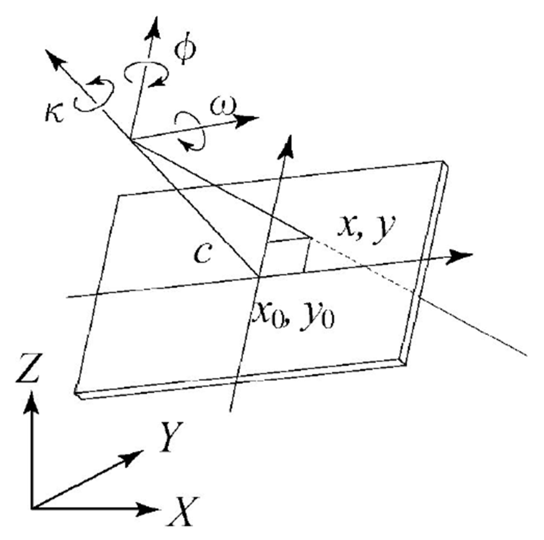
Any point P(X, Y, Z) in the spatial coordinate system is converted to P′(X′, Y′, Z′) in the image space coordinate. According to the rotation-translation formula of the space coordinate [19]:

$$\left(\begin{array}{c}{\mathrm{X}}^{\prime }\\ {\mathrm{Y}}^{\prime }\\ {\mathrm{Z}}^{\prime }\\ 1\end{array}\right)=\left[\begin{array}{c}\mathrm{R}|\mathrm{t}\\ 0 1\end{array}\right]\left(\begin{array}{c}\mathrm{X}\\ \mathrm{Y}\\ \mathrm{Z}\\ 1\end{array}\right)$$

(2)

and $\mathrm{R}={\mathrm{R}}_{\mathsf{\omega }}·{\mathrm{R}}_{\varnothing }·{\mathrm{R}}_{\mathsf{\kappa }}$, which expresses rotation.${\mathrm{R}}_{\mathsf{\omega }},{\mathrm{R}}_{\varnothing }{\mathrm{and}\mathrm{R}}_{\mathsf{\kappa }}$ are the rotation angle around the corresponding axis [20], as Figure 1 shows.

$${\mathrm{R}}_{\mathsf{\omega }}=\left(\begin{array}{ccc}1& 0& 0\\ 0& \cos \mathsf{\omega }& -\sin \mathsf{\omega }\\ 0& \sin \mathsf{\omega }& \cos \mathsf{\omega }\end{array}\right){\mathrm{R}}_{\varnothing }=\left(\begin{array}{ccc}\cos \mathsf{\varphi }& 0& \sin \mathsf{\varphi }\\ 0& 1& 0\\ -\sin \mathsf{\varphi }& 0& \cos \mathsf{\varphi }\end{array}\right){\mathrm{R}}_{\mathsf{\kappa }}=\left(\begin{array}{ccc}\cos \mathsf{\kappa }& -\sin \mathsf{\kappa }& 0\\ \sin \mathsf{\kappa }& \cos \mathsf{\kappa }& 0\\ 0& 0& 1\end{array}\right)$$

(3)

t represents translation, (0, 0, h) represents the coordinates of the camera lens center in the spatial coordinate system. According to

$$\mathrm{t}=-\left[\begin{array}{c}0\\ 0\\ \mathrm{h}\end{array}\right]$$

(4)

where h is the vertical height from the water surface. In order to obtain this height quickly, the inclination angle (α) of the device is taken as 0. As Figure 2 shows, F is the position of the optical center of the lens of the smartphone, the dotted line is the main optical axis, M and N are the upper and lower endpoints of the viewing angle, A and B are the two endpoints of the imaging object, respectively, C and D are the imaging positions of A and B in the image, and h is the elevation difference from the lens to the river surface.

Selecting table tennis as the imaging object, the diameter of the table tennis is 40 mm, that is, the distance of AB is 40 mm. the parameter h can be obtained from the following geometric formula:

$$\mathrm{h}=\mathrm{AB}\times \frac{{\mathrm{n}}^2-\mathrm{n}\tan (\mathsf{\alpha })\tan (\mathsf{\beta })\left({\mathrm{P}}_{\mathrm{A}}+{\mathrm{P}}_{\mathrm{B}}-2\mathrm{n}\right)+\left({\mathrm{P}}_{\mathrm{A}}-\mathrm{n}\right)\left({\mathrm{P}}_{\mathrm{B}}-\mathrm{n}\right){\tan }^2(\mathsf{\alpha }){\tan }^2(\mathsf{\beta })}{\left({\mathrm{P}}_{\mathrm{B}}-{\mathrm{P}}_{\mathrm{A}}\right)\times \mathrm{n}\times \tan (\mathsf{\beta })\times {\sec }^2(\mathsf{\alpha })}$$

(5)

It is easy to get the pixel coordinates of points A and B, which are P_A and P_B, respectively. The camera’s perspective 2β can be obtained, and the 2n is the total pixels in the perspective are easily known.

After transforming into the image–space coordinate system, through the conversion relationship between the image plane coordinate and image space coordinate, the corresponding point in the image plane coordinate is determined according to the principle of pin-hole imaging, as shown in the following Figure 3.

According to the side projection rule and the triangle similarity principle, the conversion relationship of the corresponding point can be obtained.

$$\left(\begin{array}{c}\mathrm{x}\\ \mathrm{y}\end{array}\right)=-\mathrm{f}\left(\begin{array}{c}\frac{{\mathrm{X}}^{\prime }}{{\mathrm{Z}}^{\prime }}\\ \frac{{\mathrm{Y}}^{\prime }}{{\mathrm{Z}}^{\prime }}\end{array}\right)$$

(6)

Through Equation (6), the coordinate of P(x,y) in distance unit can be acquired. In order to get the coordinate P(x₀,y₀) in the two-dimensional image plane, the magnification ratio [21], which is the transformation rate from the coordinate of the pixel to the ground coordinate, must be introduced. The magnification ratio plays an intermediary role in the transformation from the coordinate of the pixel to the ground coordinate. The distance in pixel can be transformed into the real distance through the magnification ratio. In order to compute the magnification ratio (e), the pixels specified by the user in the image have to be back-projected to the ground.

Computing the magnification ratio: Assume that the relationship between the real distance of two pixels and their corresponding pixel distance is linear. For two pixels P_A and P_B, their real distance, L_AB, can be estimated from their pixel distance, L_P, via a linear model with a parameter e, called magnification ratio

$${\mathrm{L}}_{\mathrm{A}\mathrm{B}}=\mathrm{e}\times {\mathrm{L}}_{\mathrm{P}}$$

(7)

In order to get the e fast and easily, the L_AB is represented by the diameter of the table tennis (40 mm), and the L_P can be calculated by the line calculation formula in the pixel coordinate. So, the magnification ratio can be estimated, and the transformation relationship of the coordinate of P(x,y) is:

$$\begin{array}{c}\mathrm{x}=\mathrm{e}\times {\mathrm{x}}_0\\ \mathrm{y}=\mathrm{e}\times {\mathrm{y}}_0\end{array}$$

(8)

2.3. Surface Velocity Calculation

The images were recorded by the smartphone (iPhone 6s) at 5 hertz, whose property is shown in

Table 1. The parameters of the smartphone (iPhone 6s).

Smartphone Property
Screen size	4.7 inches
Screen ratio	16:9
Resolution	1334 × 750 pixel

. Moreover, the corresponding magnification ratio is about 0.0078 through Equation (7) computing. After finishing the identification of the tracer and the completion of the centroid coordinate transformation, the coordinates of the tracer in space can be obtained, which means that the moving distance of the tracer can be calculated easily by the distance formula. The time interval t of each image is 0.2 s. With Equation (9), average velocity would be calculated in any time period.

$$\mathrm{v}=\frac{\mathrm{L}}{\mathrm{t}}$$

(9)

where L is the moving distance of the tracer and t is the time interval.

In the calculation process, the following assumptions were made:

• The surface of the river is horizontal and coincides with the spatial coordinate system when Z = 0.
• The center of the camera lens coincides with the Z-axis in space coordinate system and it is fixed, so the coordinate of the center of the lens is (0, 0, h). h is the distance from the center of the lens to the water surface, which needs to be manually inputted before the measurement is started.
• Lens imaging approximates the principle of pin-hole imaging.
• The effect of lens distortion on measurement accuracy is negligible.
• The selected tracers have strong fluidity along with river flow and will not disturb the surface flow.

3. Measurement Validation

3.1. Device Calibration

Before the measurement experiments are carried out, the measurement device should be calibrated, which means that the allowable pitch of angle must be guaranteed in the process of measurement. In order to attain the allowable pitch of angle easily and fast, the actual value of the experimental velocity was constant, and the elevation difference h was set at 0.752 m during measurements, and then the pitch angle was changing continuously. The measurement results were shown in Figure 4. During the increase of the pitch angle, the average value of the measurement results gradually increases.

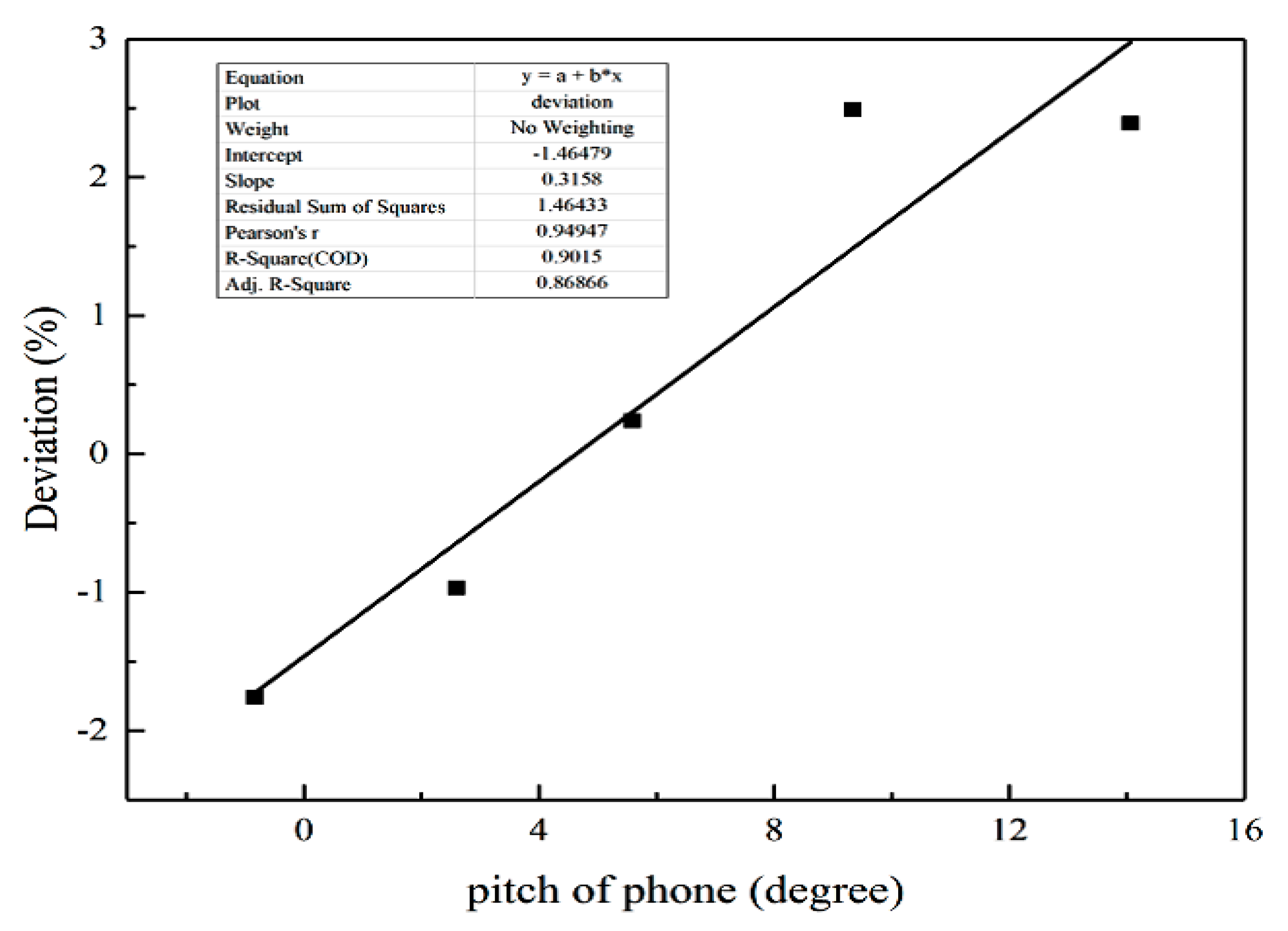
The relationship between the measurement deviation and the pitch angle is shown in Figure 5. According to the fitting result, when the relative deviation of measurement results exceeded 3%, the measured results may be invalid. So, the pitch angle should not exceed 15° when the PTV system is used. When the pitch angle is large, the amplification effect of the image resolution on the image plane coordinate exceeds the requirement. So, the experiment validation must be performed within the 15° of the pitch angle of the smartphone.

3.2. Indoor Experiment Validation

In order to verify the measurement results of the surface velocity, a comparative test was designed in the water tank experiment [22]. The elevation difference (h) of the measurement is fixed, and the actual velocity of the surface velocity is 0.02473 m/s. The measurement results through the PTV system are shown in Figure 6.

The measured values fluctuate around the actual value, and most of the measured values are close to the actual values. From the statistical results, the average of the measured values is 0.02442 m/s, and the deviation of the measurement sequence is 1.26%. Therefore, the PTV system can adapt to measurement requirements and has high measurement accuracy.

3.3. Acoustic Doppler Current Profilers (ADCP) Validation

In the ADCP system, the transmitter and receiver of the ultrasonic transducer are usually located at the same place, and there are two Doppler shifts between the transmitter (or receiver) and the suspended particles in the water. Suspended particles in the water will act as the receiver and transmitter of the sound source, respectively.

Assuming that the water velocity is v, the angle between the velocity and the sound beam is α, and the frequency of the ultrasonic wave emitted by the ADCP transmitter is f₀, the frequency received by the suspended particles in the water is:

$$f_1=\frac{c+vcos\alpha }{c}{f}_0$$

(10)

After the ultrasonic wave of frequency f₁ is reflected (or scattered), it can be considered that the ultrasonic wave is a new emission source. The suspended particles in the water are emitted. It moves at a velocity v and is received by the stationary ADCP receiver. The received frequency is:

$$f_2=\frac{c}{c-vcos\alpha }{f}_1=\frac{c+vcos\alpha }{c-vcos\alpha }{f}_0$$

(11)

Then, the Doppler frequency shift is:

$$f_d=f_2-f_0=\frac{2vcos\alpha }{c-vcos\alpha }{f}_0$$

(12)

From the above calculation, the water velocity is:

$$\mathrm{v}=\frac{c}{2f_{0}cos\alpha }\left(f_2-f_0\right)$$

(13)

During the experiment of the control group, the experimenter stands on the bank of the river next to the water surface, and the distance from the water surface was less than 5 cm. During the experiment, ensure that it was parallel to the water flow, α < 5°, and α = 0.

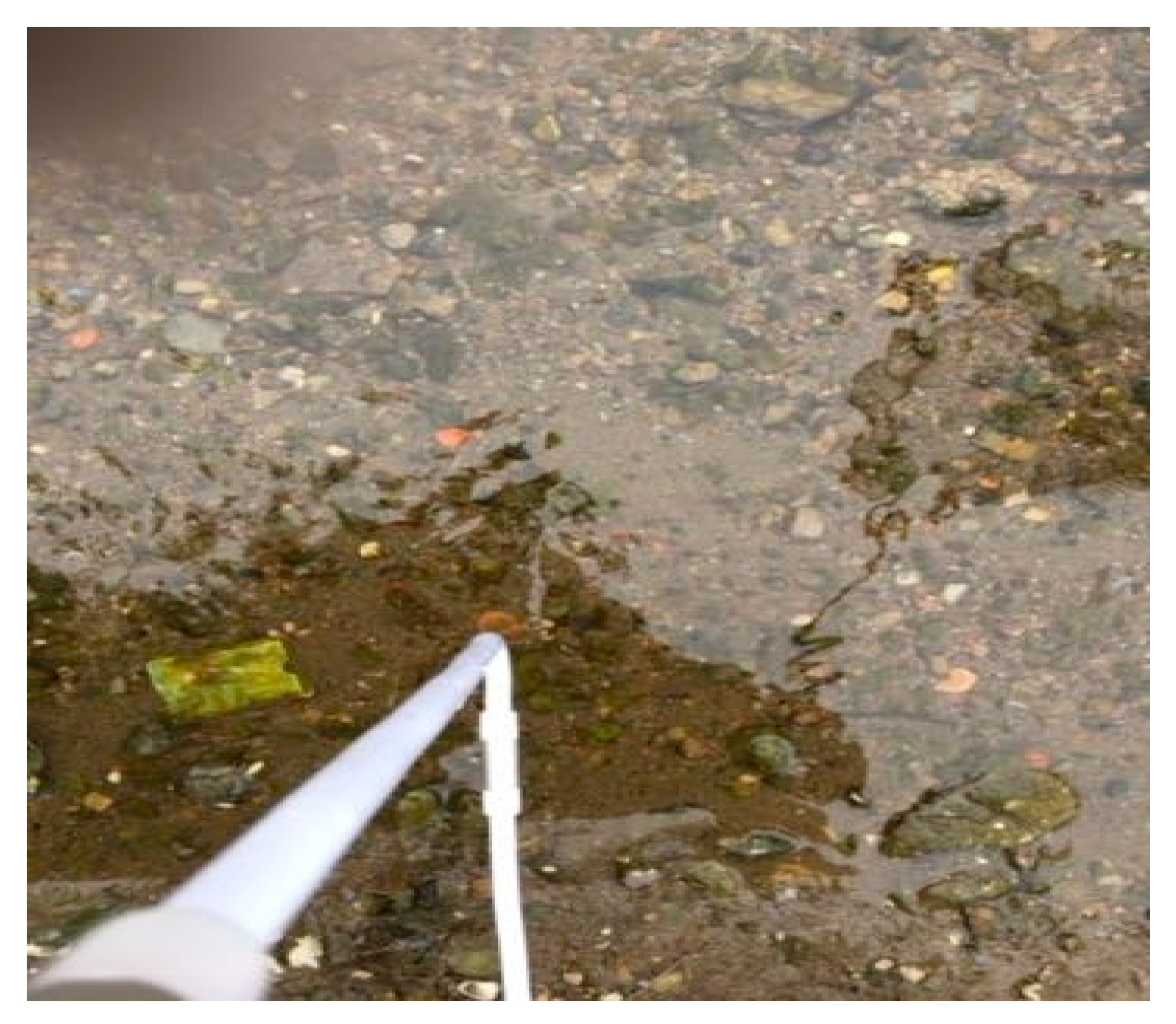
In order to test the applicability of the LSPIV, a field experiment was also carried out. A control group and an experimental group were designed. Acoustic Doppler current profilers were used in the control group and the PTV system was used in the experimental group. The experimental site was selected in the Wanquan River, downstream of the school river in the Tsinghua University. On the day of the experiment, the flow rate of the river was low and the water depth in the deepest part was no more than 20 cm. The water quality was good and fine sand can be clearly seen. There was almost no grass. The water surface width is about 5 m and the wind velocity was about 2 m/s, no creatures such as fleas can cause the failure of the ADCP [23]. The image captured by the iPhone 6s was shown in Figure 7, and the white bracket was a system-assisted device.

The measurement results by the ADCP are shown in

Table 2. The measurement results of the acoustic doppler current profilers (ADCP).

Measurement Sequence	1	2	3
Measurement value	0.21 (m/s)	0.26 (m/s)	0.22 (m/s)

. Three sets of experiments were carried out, S1, S2, and S3. The average flow rate obtained by ADCP was 0.23 m/s.

The measurement results by the PTV system are shown in Figure 8 and the average flow rate obtained by PTV was 0.262 m/s. In order to ensure the accuracy of the measurement, multiple measurements were taken. S1, S2, and S3 were three measurements series by the same measuring mean. The measurement value 0.23 m/s is the average value of three measurements by ADCP, and the measurement value 0.262 m/s is the average of three measurements by the PTV system. The result distribution of the PTV system was stable. Comparing the average of measurement results with the results by ADCP, the measurement error of the PTV system did not exceed 15%.

4. Discussion

The measurement results of the PTV are susceptible to the pitch angle and the elevation difference. In order to examine the performance of elevation difference, the actual value of the experimental velocity did not change, and the elevation difference changes continuously from small value to large value during the measuring. As the elevation difference varies, the measurement results will fluctuate. When h is too low, the image sharpness will be influenced significantly. On the other hand, when h is low, the imaging range is small, which means that the number of images captured is not enough and the measured results would be inaccurate. When h is too high, the specular reflection on the surface of the tracer causes the highlight to be too strong, affecting the recognition of the tracer, which leads to incorrect measurement results. Besides, due to the limitation of the image resolution, the number of pixels occupied by the tracer would decrease sharply, which results in measurement failure.

At the same time, the performance of the pitch angle was also verified. The actual value of the experimental velocity was constant and the elevation difference was fixed during measuring, and the pitch angle was constantly changing from the small value to the large value. With the increase of the pitch angle, the average value of the measurement results gradually increases. The reason is that when the pitch angle is large due to the limitations of image resolution and the errors in the image plane coordinate would be magnified. On the other hand, in the process of measuring, there exists the assumption that the surface of the river is horizontal. The pitch angle is equivalent to the corresponding tilt angle of the plane of motion, which means that when the pitch angle is large, the error of the measurement results would become large. So, the pitch angle should not be too large.

The applicable scope of the system is limited. The performance of the system at different actual velocities was examined under different working conditions. When the actual velocity exceeds 1.5 m/s, the relative error between the actual value and the measurement results will be more than 3%. So, the difference between measuring results and actual results is significant and the measuring results are invalid. The primary reason is that when the actual velocity is fast, which will result in the photons of the centroid point of the tracer, not the same point when they reach the film, leading to blurred images. So, the centroid point of the tracer is not capable of being captured precisely. The moving distance of the tracer is not valid and the measurement velocity is not reliable. On the other hand, the measuring frequency is set at 5 Hertz. So, the exposure time is not short and, when the measured velocity is too fast, it smears the images and the images of the captured tracer would be distorted. Therefore, it is difficult to acquire clear and high-resolution images. Based on the above reasons, the application range of the measuring system is small and the velocity of the river surface is not supposed to be fast.

5. Conclusions

Based on the basic principle of PTV technology, the new method of measurement of river surface velocity was established by means of tracer identification. The smartphone (iPhone 6s) was used to take images, which has the advantages of real-time, low cost, and portability. The system uses the corrected normalized RGB color model for tracer identification. In order to verify the accuracy, different operating conditions which included the indoor validation experiment and field validation experiment were designed. After indoor testing, the relative deviation between the average value of the measurement sequence and the true value did not exceed 3%. After the ADCP validation, the results showed that the measurement error did not exceed 15% compared to the ADCP results. Moreover, the measurement results of the PTV are susceptible to the pitch angle and the elevation difference. The pitch angle should not be too large and the elevation difference should not be too low or too high. The applicable scope of the system is limited. When the measured velocity is too fast, the measuring system will be invalid. There are also some defects in the measuring system. For instance, the modified normalized RGB color model is effective in achieving the measurement of water surface velocity in good light conditions. However, the RGB class model has poor adaptability to light changes. Consider developing a tracer recognition model that combines the contour recognition method with the normalized RGB model in the future. The modified normalized RGB color model is effective in achieving velocity measurement in good light conditions. In good light conditions, the tracer can be positioned accurately through the normalized RGB model. The RGB model has poor adaptability to light changes. When the light intensity changes, the RGB value cannot change proportionally, the normalized RGB model can only eliminate part of the light effect, and the effect of processing highlights is not good; at the same time, the processing ability on the gray type and black pixels is insufficient. Therefore, improving the image resolution is considered, which can improve the recognition of the tracer and reduce the measurement error. Besides, in order to reduce the number of calculation programs and to acquire the measuring results fast, the image preprocessing is ignored. In future research, the image preprocesses will be considered to improve the accuracy of measurement results.