Discrepancies on Storm Surge Predictions by Parametric Wind Model and Numerical Weather Prediction Model in a Semi-Enclosed Bay: Case Study of Typhoon Haiyan

Abstract

This study explores the discrepancies of storm surge predictions driven by the parametric wind model and the numerical weather prediction model. Serving as a leading-order storm wind predictive tool, the parametric Holland wind model provides the frictional-free, steady-state, and geostrophic-balancing solutions. On the other hand, WRF-ARW (Weather Research and Forecasting-Advanced Research WRF) provides the results solving the 3D time-integrated, compressible, and non-hydrostatic Euler equations, but time-consuming. To shed light on their discrepancies for storm surge predictions, the storm surges of 2013 Typhoon Haiyan in the Leyte Gulf and the San Pedro Bay are selected. The Holland wind model predicts strong southeastern winds in the San Pedro Bay after Haiyan makes landfall at the Leyte Island than WRF-ARW 3 km and WRF-ARW 1 km. The storm surge simulation driven by the Holland wind model finds that the water piles up in the San Pedro Bay and its maximum computed storm surges are almost twice than those driven by WRF-ARW. This study also finds that the storm surge prediction in the San Pedro Bay is sensitive to winds, which can be affected by the landfall location, the storm intensity, and the storm forward speed. The numerical experiment points out that the maximum storm surges can be amplified by more 5–6% inside the San Pedro Bay if Haiyan’s forward speed is increased by 10%.

1. Introduction

Storm surges caused by tropical storms can have a significant impact on coastal facilities [1]. In some cases, storm surges can interact with tides [2,3] and wind waves [4,5,6]. When a storm approaches coastal regions, winds can amplify the height of storm surges locally at least two times more than that in the open ocean [5,6]. Hence, to perform an accurate storm surge modeling, having a better understanding of storm-wind fields is critical.

In the Western Pacific Ocean, more intense typhoons potentially occur in the future and the low-lying regions become more vulnerable to storm surges [7,8]. To minimize the disaster of storm surges, the accuracy of predicting storm surges needs to be improved. The uncertainties of storm surge predictions can attribute to the input data (e.g., bathymetry and winds), physics consideration (coupling with waves, tides, river flows, etc.), and numerical settings (e.g., grid size, time step, and an algorithm of the model discretization). However, the most variable factor should be storm wind, which accuracy depends on the storm track, the storm intensity, and the forward speed of a storm [9].

Storm-wind fields can be acquired from either a numerical weather prediction (NWP) model or a parametric wind (PW) model to drive storm surge models. The NWP models such as WRF (weather research and forecasting [10]), CReSS (cloud resolving storm simulator [11]), and ECMWF (European Centre for Medium-Range Weather Forecasts [12]), are widely used in storm surge modeling (see, e.g., [13]). NWP models solve the 3D time-integrated, compressible, and non-hydrostatic Euler equations and consider more complicated physical mechanisms (e.g., the land topography effect). However, NWP models become extremely time-consuming once a finer grid or a larger domain is required. Besides, the grid size of NWP models is vital in the tropical storm modeling [14,15].

Besides NWP models, PW models provide other standard options in storm surge forecasting [16,17], hindcasting [18,19,20], or flood risk assessment [21]. Some conventional PW models are the modified Rankine vortex model [22], SLOSH (Sea, Lake, and Overland Surges from Hurricanes) wind model [23], and Holland wind model [24]. Storm pressure and wind fields are conveniently reconstructed by the parameters: locations of storm center, the central pressure of a storm, the maximum wind speed, and the radius of maximum wind [24,25,26]. Hence, the accuracy of reconstructed parametric storm wind fields is highly dependent on these input parameters [18,27]. Furthermore, by considering a forward storm motion, the symmetric shape of storm winds can be modified [23]. However, PW models neglect physical mechanisms such as storm-topography interactions and assume to be frictional-free. Compared to NWP models, PW models are economical solutions and can serve as first-order storm wind predictive tools.

Since both NWP and PW models have their own limitations to reconstruct storm-wind fields, the trade-off solutions, hybrid-type storm wind fields, are used for storm surge [28] and wind wave modeling [29]. Storm wind fields can be acquired by combing the winds from NWP and PW models using some coefficients. However, these coefficients need to be tested and are not guaranteed to be appropriate for every typhoons’ situation. This solution is beyond the scope of this study.

Despite the discrepancies of storm surge modeling using different PW models has been widely discussed [9,27,30], the differences of storm surge predictions between PW and NWP models are relatively less explored, especially in the Western Pacific Ocean. Hence, for the storm surge modeling in the Western Pacific Ocean, understanding the differences resulted from the wind fields of the PW and NWP models is necessary.

To shed more light upon the discrepancies of storm surge modeling driven by NWP and PW models, a case study of Typhoon Haiyan is considered. Typhoon Haiyan, also known as its local name Yolanda, was the strongest storm in 2013, struck the Philippines with catastrophic storm surges, winds, and waves, and caused casualties more than 6300 [31]. The event of Typhoon Haiyan has three uniqueness: (1) the record-breaking wind speed; (2) the fast storm’s forward motion; and (3) the notable induced storm surges. First of all, Haiyan has a record-breaking intensity, sustained wind speed of more than 310 km/h [7]. Haiyan first made landfall at the southeast of the Samar Island at 4:40 a.m. 8 November 2013 (local Philippines time) with its peak intensity, made the second landfall at Dulag, Leyte at around 7:00 a.m. 8 November 2013 (local Philippines time), and then passed over the Leyte Island and the Cebu Island. Secondly, Haiyan’s forward speed can reach up to 41.0 km/h, which was more than twice over the average forward speed of tropical cyclones in the mid-latitude regions from 1951 to 2012 [32]. Lastly, because of the storm track and the landfall location of Haiyan, the most damaged regions by storm surges were found in the Leyte Gulf and the San Pedro Bay [33,34,35,36]. This uniqueness makes Typhoon Haiyan become a good case study for highlighting the discrepancies of storm surge predictions by storm winds in the Western Pacific Ocean.

Several studies have analyzed Haiyan’s storm surges numerically. The peak frequency of storm surges caused by Haiyan is comparable to the first mode of the seiche oscillation in the Leyte Gulf, which can amplify the surge heights [13]. The wind drag coefficient and the radius of maximum wind (RMW) are sensitive to the storm surge prediction using a surge-wave coupling model [18]. Three sequences of storm surges hit Tacloban in the San Pedro Bay are indicated, which correspond to the eyewitness report [35]. By using ensemble simulations with regional climate models, storm surges in the Leyte Gulf caused by the worst-case scenario can potentially be worse by 20% [37]. The storm forward speed and the storm track have been proved that they are essential to generate significant storm surges in the San Pedro Bay [19,38]. These studies pave the way on exploring the storm surges caused by Haiyan from different points of view.

The shallow water equations (SWE) model has been used to simulate storm surges successfully from open ocean to coastal regions [2,5,6,30,39]. By integrating flow properties from the sea bottom to the water surface, the depth-averaged flow velocities and free surface elevations are solved in the assumption of long wave. By neglecting the advection terms in the momentum conservations [23,40], the linear shallow water equations (LSWE) model such as SLOSH [23] becomes an economic tool in predicting storm surges. Besides traditional SWE models, some sophisticated numerical models such as non-hydrostatic wave models [20,41] can be used in the storm surge modeling as well. However, they may be more time-consuming than traditional SWE models if similar spatial resolutions are required. Moreover, LSWE models have been used to study Haiyan’s storm surges [42,43]. By considering the balance between efficiency and accuracy, the LSWE storm surge model will be used to predict storm surges induced by Typhoon Haiyan in this study.

In this study, by using the storm surge model solving LSWE, the discussions focus on the storm surges in the Leyte Gulf and the San Pedro Bay in the Philippines, which were extremely damaged by Haiyan. Both PW and NWP models are used to drive the storm surge model. The PW model results are from the widely-used Holland wind model [24]. The well-known Weather Research and Forecasting-Advanced Research WRF (WRF-ARW) model provides the results of the NWP model.

This paper is organized as follows. In Section 2, we first present the storm surge model used in this study. Then, the parametric Holland model and the WRF-ARW model are elaborated. In Section 3, the discrepancies in the modeling of Haiyan between the parametric Holland model and WRF-ARW are discussed. Afterward, the numerical experiments focused on a storm forward motion is carried out. In Section 4, we conclude this study and give some suggestions for future studies.

2. Methodology

2.1. Storm Surge Model

In this study, the depth-integrated storm surge model solving the set of linear shallow water equations with the Coriolis effect and the bottom friction is adopted. This storm surge model is based on the COMCOT (COrnell Multi-grid COupled Tsunami) tsunami model. COMCOT has been validated by the solitary wave run-up benchmark problem [44] and been used to study tsunami events such as 1960 Chilean Tsunami [45], 2004 Indian Ocean Tsunami [46,47] and 2011 Japan Tohoku Tsunami [48]. Furthermore, COMCOT has been developed into a cloud computing platform [48]. The external forcing terms of the sea-level pressures and the wind shear stresses are added to the momentum equations of COMCOT to simulate the storm surge propagation.

The mass and momentum equations of the linear shallow water equations in the Cartesian coordinate are presented as follows:

$$\frac{\partial \eta }{\partial t}+\frac{\partial P}{\partial x}+\frac{\partial Q}{\partial y}=0,$$

(1)

$$\frac{\partial P}{\partial t}-fQ=-gH\frac{\partial \eta }{\partial x}-\frac{H}{{\rho }_w}\frac{\partial P_a}{\partial x}+\frac{{\tau }_{sx}}{{\rho }_w}-\frac{{\tau }_{bx}}{{\rho }_w},$$

(2)

$$\frac{\partial Q}{\partial t}+fP=-gH\frac{\partial \eta }{\partial y}-\frac{H}{{\rho }_w}\frac{\partial P_a}{\partial y}+\frac{{\tau }_{sy}}{{\rho }_w}-\frac{{\tau }_{by}}{{\rho }_w},$$

(3)

where $\eta$ is the water surface elevation, $t$ is the time, $x$,$y$ are spatial notations, ($P$,$Q$) are the depth-integrated volume fluxes per unit length, $H$ is the total water depth ($H=h+\eta$), $h$ is the still water depth, g is the gravitational acceleration (=9.81 m/s²), $f$ is the Coriolis parameter ($f=2\omega sin\phi$), $\omega$ is the Earth angular velocity (=7.2921 × 10⁻⁵ rad/s), (${\tau }_{sx}$, ${\tau }_{sy}$) are the wind shear stresses, (${\tau }_{bx}$, ${\tau }_{by}$) are the bottom frictional shear stresses, ${\rho }_w$ is the water density (=1000 kg/m³), and $P_a$ is the sea-level air pressure.

The Manning’s formula, originally from the conception of the open-channel flow, is used to model the bottom friction:

$${\tau }_{bx}={\rho }_w\frac{g{n}^2}{H^{7/3}}P\sqrt{\left(P^2+Q^2\right)},$$

(4)

$${\tau }_{by}={\rho }_w\frac{g{n}^2}{H^{7/3}}Q\sqrt{\left(P^2+Q^2\right)},$$

(5)

where $n$ is the Manning’s roughness coefficient. By introducing appropriate Manning’s coefficient, the roughness of the material can be determined in this formula. As shown in Equations (4) and (5), the bottom friction is proportional to the squared of volume fluxes per unit length and the Manning’s coefficient and inversely proportional to the water depth to the power of 7/3. Hence, the bottom friction using this formula is less important in deep waters, more significant in shallow waters, and crucial in coastal regions (including inland areas). Since the inundation calculation is not involved in this study, the Manning’s coefficient is 0.025 over the whole computational domain, which is also adopted by other studies [18,19]. In fact, the Manning’s coefficient shall be determined carefully, especially the inundation calculation involved. The use of the Manning’s roughness coefficient to storm surge modeling has been investigated [49,50,51].

The quadric law is used to model the wind shear stresses on the water surface:

$${\tau }_{sx}={\rho }_a{C}_d{u}_{10}{u}_{10x},$$

(6)

$${\tau }_{sy}={\rho }_a{C}_d{u}_{10}{u}_{10y},$$

(7)

in which $C_d$ is the wind drag coefficient between the water surface and the air, $u_{10}$ is the 10-m wind speed, ($u_{10x}$, $u_{10y}$) are the components of the 10-m wind speed in the x- and y-directions. The wind drag coefficient of Wu (1982) is used [52]:

$$C_d=\{\begin{array}{c}\hspace{1em}\hspace{1em} 1.2875\times {10}^{-3}, u_{10}<7.5,\\ \left(0.8+0.065\right)\times {10}^{-3}, u_{10}\ge 7.5.\end{array}$$

(8)

The boundary conditions along the computational domain are given by the free surface elevations caused by the pressure drop (i.e., the difference between the sea-level pressure and the ambient pressure) in wet cells:

$$\eta =-\frac{\Delta p}{\rho g}.$$

(9)

This storm surge model is discretized by the explicit finite difference method in time and space. The leap-frog scheme is used to discretize the free surface elevation at (n + 1/2)Δt and the volume fluxes per unit length at (n + 1)Δt [53,54]. The forward finite difference method is used to solve the mass equation and the momentum equations. The staggered grid system, Arakawa C grid, is used [55]. Hence, the volume fluxes are defined at the boundaries of cells and the free surface elevations are in the center of cells. The boundary conditions between wet and dry cells are non-flux boundary conditions. It implies the volume fluxes of water cannot go across the coastline (i.e., the inundation calculation is not considered and the coastline is fixed in the simulation). Hence, the mass conservation is solved only in wet cells.

The tide effect and its interaction with storm surges are not considered in this study because the predicted tidal level was 0.15 m (about 2–3% of the peak surge) when the peak surge occurred at 00:00 UTC 8 November 2013 [13,18] and the maximum tidal range was within 1.0 m in the San Pedro Bay [35]. The wave radiation stresses are not considered since they are insignificant in generating storm surges along the coasts of the Leyte Gulf [13,56] and the maximum wave-enhanced storm surge is about 0.3 m (approximately 6% of the peak storm surges) at Tacloban.

2.2. Parametric Holland Wind Model

In this study, the well-known parametric Holland wind model (hereafter, HWM), is adopted to reconstruct the meteorological fields of Typhoon Haiyan. HWM has been widely used in storm surge modeling and wind-wave modeling [30,57]. The exponential distribution of the atmospheric pressure proposed by Schloemer (1954) [58] is extended by Holland (1980) [24]:

$$P_a\left(r\right)=P_c+\Delta P\times exp\left[-{\left(\frac{R_{max}}{r}\right)}^B\right],$$

(10)

where $P_c$ is the central storm pressure, $\Delta P$ is the pressure drop ($\Delta P=P_n-P_c$), $P_n$ is the ambient pressure, $R_{max}$ is the radius of maximum wind, $r$ is the distance from the specified grid to the storm center, and $B$ is the scaling parameter. Note that $P_n$ can vary in the regions from about 1010 to 1013.25 hPa [59]. For the sake of simplicity, $P_n$ = 1013.25 hPa is used in this study.

By using the gradient wind balance equation, the solution of the radial wind profile with the Coriolis effect is yielded [24,60]:

$$V_g\left(r\right)=\sqrt{{\left(\frac{R_{max}}{r}\right)}^B\times \frac{B\Delta P\times exp\left[-{\left(\frac{R_{max}}{r}\right)}^B\right]}{{\rho }_a}+{\left(\frac{rf}{2}\right)}^2}-\frac{rf}{2}.$$

(11)

$V_g$ is the computed gradient Holland wind speed. Note that this solution is steady axisymmetric and geostrophic. The maximum gradient wind speed exists where r = R_max where the Coriolis force is relatively insignificant compared to the pressure gradient and the centrifugal force,

$$V_{g,max}=\sqrt{\frac{B\Delta P}{{\rho }_{a}e}}.$$

(12)

As shown in Equation (12), the maximum gradient wind speed is proportional to the square root of the scaling parameter B, and the pressure drop $\Delta P$.

The 1999 Harper and Holland’s scaling parameter B for the computed pressure and wind profiles is shown below [60]:

$$B=2-\frac{P_c-900}{160},$$

(13)

where the scaling parameter B is limited from 1.0 to 2.5. Note that if the scaling parameter B = 1, the pressure distribution proposed by Schloemer (1954) [58] is assumed.

The radial distribution of the wind speed from the storm center is already given by Equations (10)–(13). Now, the wind directions are needed to define. As the assumption of a steady axisymmetric storm, the wind direction is cyclonic toward the storm center. However, while the storm is moving forward, the wind flows are crossing the isobars [60,61], which indicates an inward angle shall exist. In this study, the inward angle of 25 degrees is used [62]. By adopting the assumption of the cyclonic winds toward a storm center and the inward angle deviating from the isobars, the vector form of the gradient winds ${\mathit{V}}_{\mathit{g}}$ is yielded from the function form of Equation (11).

The correction factor is introduced here to convert the computed gradient Holland wind speed to the wind speed on the standard level, the 10-m height above the mean sea-level:

$${\mathit{V}}_{\mathit{m}}=K_m{\mathit{V}}_{\mathit{g}},$$

(14)

where K_m is based on the logarithmic law,

$$K_m=\frac{\ln \left(10/z_0\right)}{\ln \left(z_g/z_0\right)},$$

(15)

in which $z_0$ is the roughness length and $z_g$ is the height of the gradient wind. However, $z_0$ and $z_g$ are hard to define during intense tropical storms. Alternatively, $K_m$ can be approximately used as 0.7 for the 10-m wind conversion of the Holland wind model [60]. Further discussions of K_m on storm surge and wind wave modeling can be found in the studies such as Chueng et al. (2003) [30] and Phadke et al. (2003) [57].

While a storm is moving, the wind pattern becomes asymmetric because winds are amplified on the right and weaken on the left in a storm forward direction. The correction term for an asymmetric wind pattern is proposed [23]:

$${\mathit{U}}_{\mathit{c}\mathit{o}\mathit{r}}\left(r\right)=\frac{R_{max}r}{R_{max}{}^2+r^2}{\mathit{V}}_{\mathit{f}}.$$

(16)

${\mathit{U}}_{\mathit{c}\mathit{o}\mathit{r}}$ is the correction term and ${\mathit{V}}_{\mathit{f}}$ is the forward velocity of a storm. The maximum corrected term exists where r = R_max and is equivalent to the half of the forward storm velocity.

Finally, by assuming the exponential pressure distribution with the scaling parameter, using the gradient wind balance equation, and considering the effect of the storm forward motion, the 10-m winds are expressed by

$${\mathit{U}}_{\mathbf{10}}=K_m{\mathit{V}}_{\mathit{g}}+{\mathit{U}}_{\mathit{c}\mathit{o}\mathit{r}}.$$

(17)

Note again that the 10-m winds come from the parametric wind model used in this study are frictional-free, steady-state, and geostrophic-balancing solutions.

2.3. WRF-ARW Model

In this study, the 10-m wind fields and sea-level pressures performed by the WRF-ARW (Weather Research and Forecasting-Advanced Research WRF) model are involved. WRF-ARW solves the 3D time-integrated, compressible, and non-hydrostatic Euler equations [10]. The model results of WRF-ARW version 3.8.1 used in this study are Cases 3 km F2 and 1 km F2 of Kueh et al. (2019) [15]. They will be denoted as WRF-ARW 3 km and WRF-ARW 1 km in the following discussion. The horizontal domain of WRF-ARW is from (117.88° E–147.12° E) and (0.0° N–19.62° N), and 45 vertical levels are employed. More modeling details and numerical settings of WRF-ARW can be found in Kueh et al. (2019) [15].

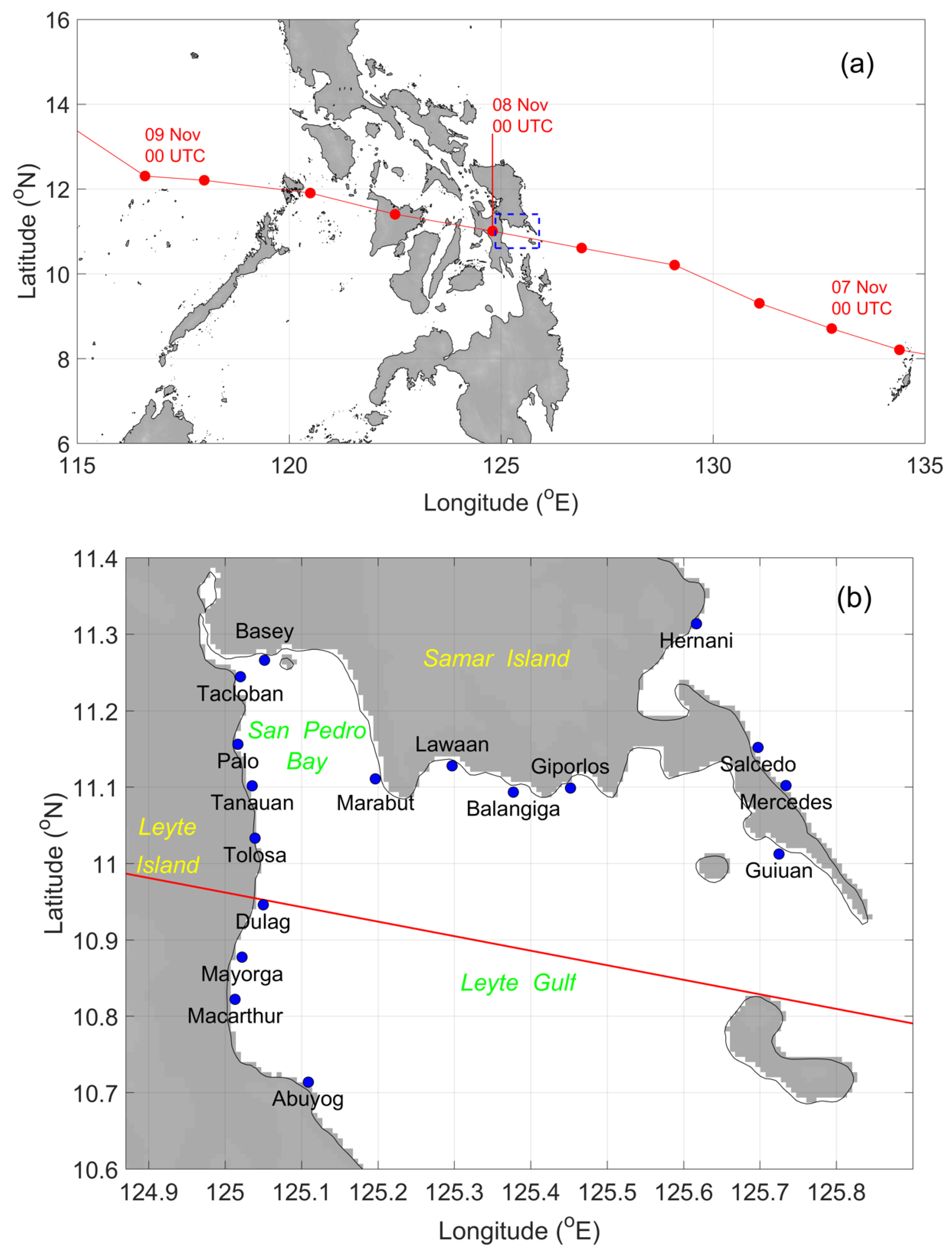
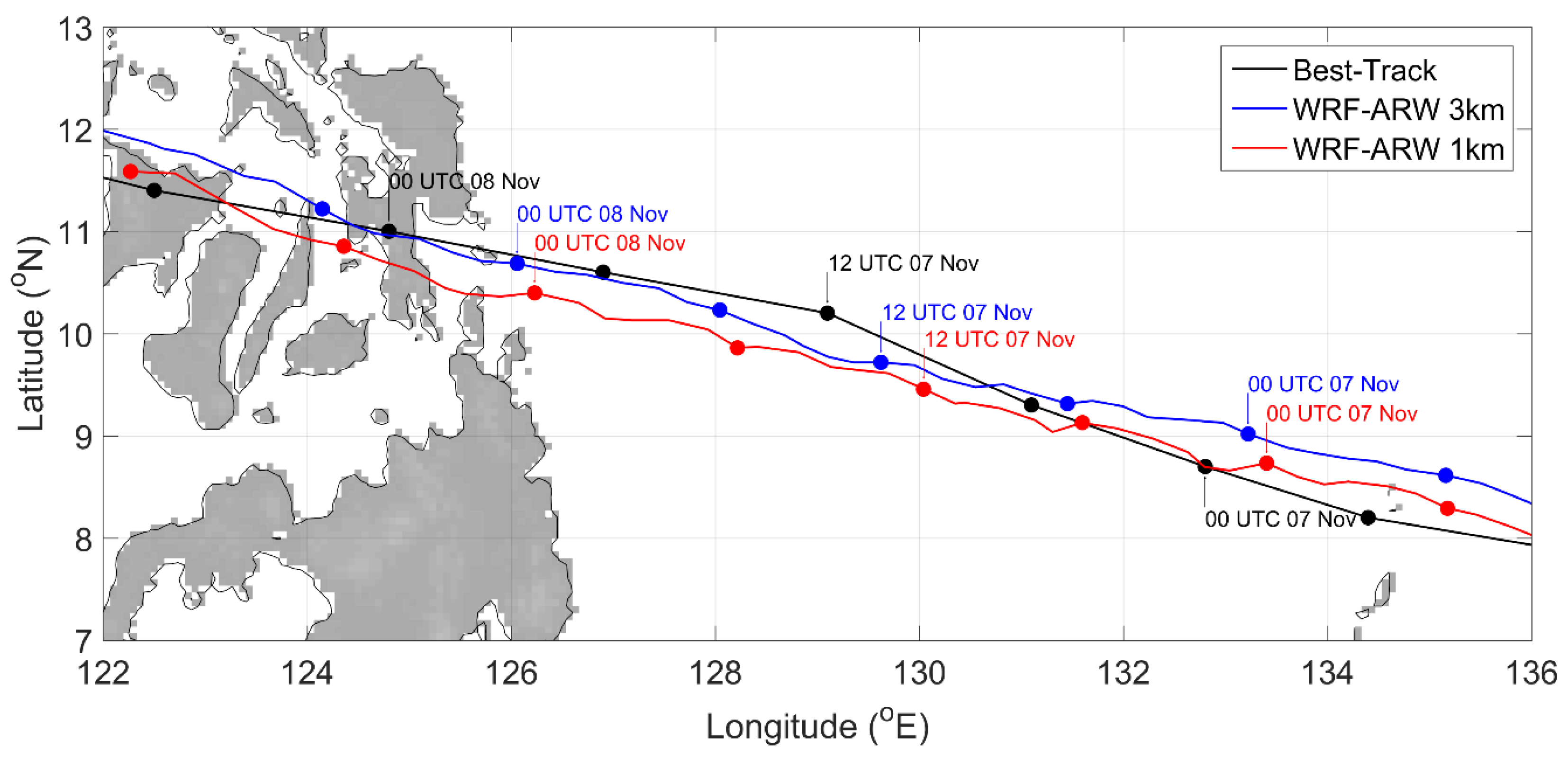
2.4. Storm Track and Parameters of Haiyan

The storm track of Haiyan is illustrated in Figure 1a, and the best-track parameters from the JMA (Japan Meteorological Agency) database [63] are listed in

Table 1. Strom track parameters of 2013 Typhoon Haiyan from the JMA best-track database, provided in every 6 h. In this table, the maximum wind speeds of Haiyan are converted to the SI unit, m/s. The time zone of this table is UTC + 0 time. P_c indicates the central pressures of Haiyan, and V_max depicts the maximum sustained wind speeds.

Year	Month	Day	Hour	Longitude (° E)	Latitude (° N)	Pc (hPa)	Vmax (m/s)
2013	11	6	18	134.4	8.2	905	59.16
2013	11	7	00	132.8	8.7	905	59.16
2013	11	7	06	131.1	9.3	905	59.16
2013	11	7	12	129.1	10.2	895	64.30
2013	11	7	18	126.9	10.6	895	64.30
2013	11	8	00	124.8	11.0	910	56.58
2013	11	8	06	122.5	11.4	940	46.30
2013	11	8	12	120.5	11.9	940	46.30
2013	11	8	18	118.0	12.2	940	46.30
2013	11	9	00	116.6	12.3	940	46.30

. The JMA best-track database provides the best-track parameters of a storm every 6 h, such as the central pressures, the maximum sustained wind speeds, and the locations of a storm center. As shown in Figure 1a, Typhoon Haiyan passed over the central regions of the Philippines and made landfall at the Samar and Leyte Islands between 18:00 UTC 7 November 2013 and 00:00 UTC 8 November 2013. In Figure 1b, Haiyan passed over the Leyte Gulf and the San Pedro Bay. From the best-track parameters listed in Table 1, Haiyan has the lowest central pressure of 895 hPa and sustained wind speed of about 64.30 m/s at 12:00 UTC and 18:00 UTC 7 November 2013. It implies that Haiyan made landfall in the Philippines while it has a peak storm intensity.

The parameters required in HWM have been described in Table 1, except for the radius of the maximum wind (RMW, R_max). RMW is an important parameter which decides the scale of the storm winds. The effect of R_max to storm surge modeling has been investigated by Kim et al. (2015) [18] and R_max of 50 km with the leveling-off drag coefficient fulfills the survey data. However, smaller R_max (accurately, R_max = 23 and 30 km) is used to perform the storm surge simulation of Haiyan by Kumagai et al. (2016) [19]. However, the pressure distributions used in Kim et al. (2015) and Kumagai et al. (2016) are different from the one in this study. Therefore, RMW shall be examined again. In the following section, the effect of RMW will be discussed and verified against the observed weather data at the Guiuan weather station.

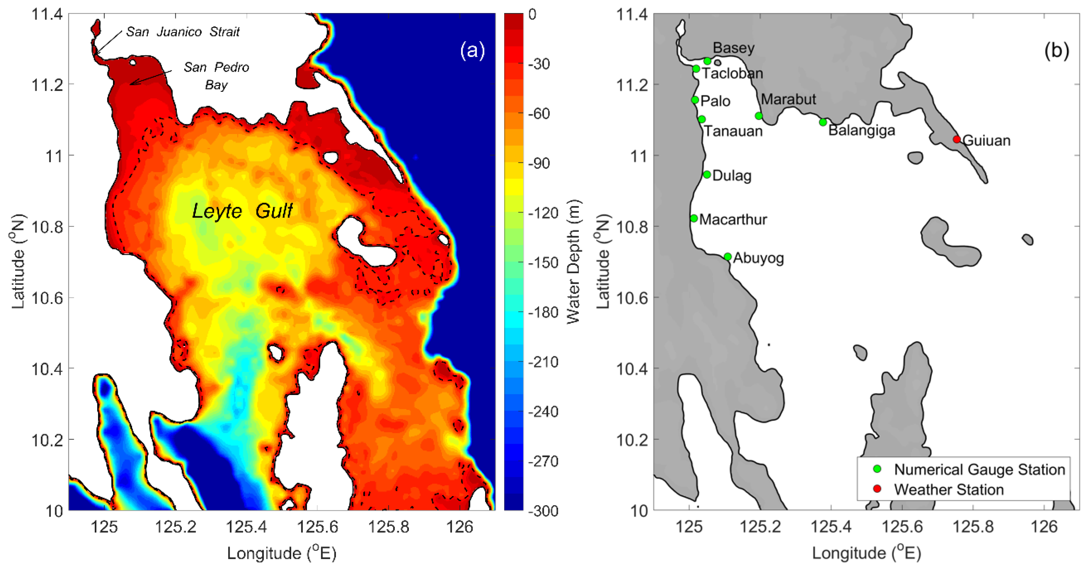
2.5. Computational Setup of Storm Surge Modeling

The computational domain of the storm surge model is shown in Figure 2a. The domain is designed to study the storm surges induced by Haiyan in the Leyte Gulf and the San Pedro Bay where had been impacted dramatically. The model domain is from (124.9° E–126.1° E) and (10.0° N–11.4° N). As shown in Figure 2a, the coastline along the Samar Island to the Leyte Island is similar to the funnel shape, which makes this region more susceptible to storm surges [35]. In the San Pedro Bay, the water depths are less than 30 m, which depicts that the wind shear stresses can play an important role in intensifying storm surges locally. The source of the bathymetry is from GEBCO (the GEneral Bathymetric Chart of the Oceans) 2014 grid [64]. The grid size of the computational domain is 277.7 m over the whole computational domain. The model time step is 0.5 s to fulfill the Courant–Friedrichs–Lewy (CFL) condition in the explicit finite difference model [65]. The storm surge simulations are performed from 00:00 UTC 7 November 2013 to 12:00 UTC 8 November 2013, a total of 129,600 s. In our study, because of insufficient information of bathymetry and land data for the San Juanico Strait, our simulations end in the frontal part of the strait (see Figure 2a) and the boundary condition used is non-flux. The storm surges induced by Haiyan around the San Juanico Strait have been discussed by Bricker et al. (2014) [66]. They indicated that Haiyan’s storm surges can extend up from the San Pedro Bay through the San Juanico Strait to Bogulibas and rapidly dissipate where the strait narrows. Note that the results reached by Bricker et al. (2014) [66] were based on the simulations using rough bathymetry from GEBCO and topography from SRTM (Shuttle Radar Topography Mission) despite some local detailed data such as the nautical charts were adopted. The results are expected to be better if more accurate bathymetry and land data can be acquired in future works.

The time histories of storm surges are provided at the specified numerical gauges in the storm surge model. Figure 2b shows the map of these numerical gauges, and

Table 2. Locations of the numerical gauges setting in the storm surge model.

Station Name	Longitude (° E)	Latitude (° N)
Balangiga	125.3775	11.0934
Marabut	125.1968	11.1108
Tacloban	125.0199	11.2440
Tanauan	125.0356	11.1014
Basey	125.0518	11.2657
Dulag	125.0500	10.9458
Abuyog	125.1089	10.7137
Palo	125.0168	11.1560
Macarthur	125.0132	10.8221

lists their locations. Note again that the boundary conditions between wet and dry cells are non-flux (i.e., the volume fluxes of water are not allowed to cross the coastline and set to zero along the coastline). Hence, the locations of the numerical gauges are moved two to three grids away from the coastline to avoid the land effect caused by the boundaries.

3. Results and Discussions

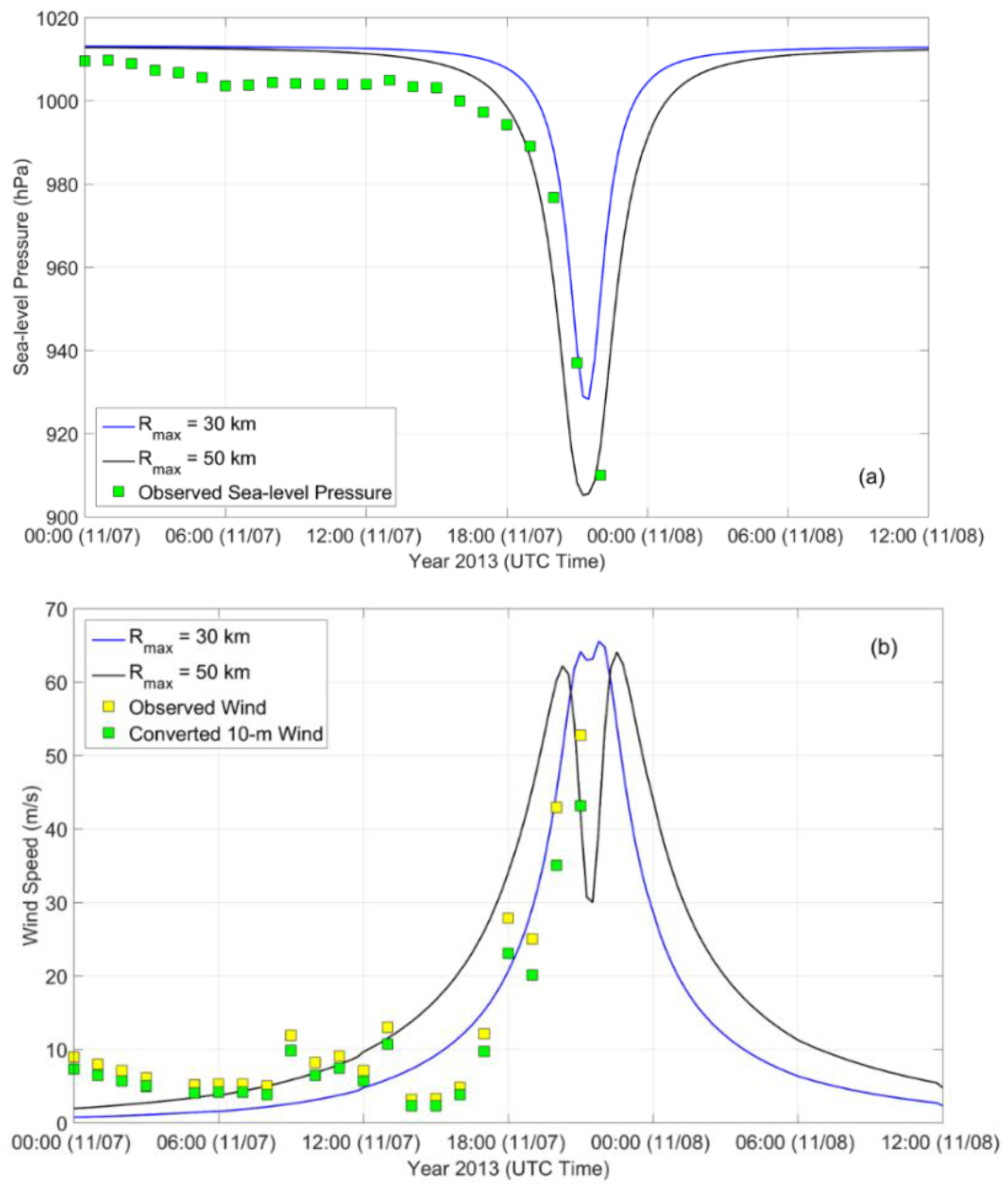
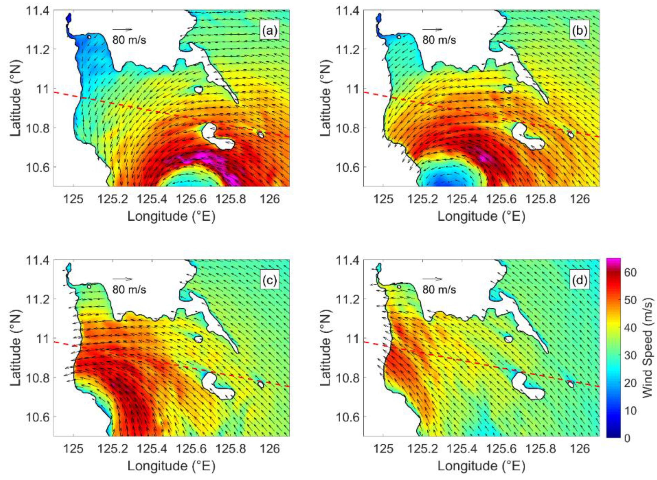
3.1. Validation of Parametric Holland Wind Model

Before performing the storm surge simulation, the results of HWM shall be verified. Hence, in this section, the 10-m winds and the sea-level pressures of HWM are compared to the observed data at the Guiuan weather station, East Samar. In the Guiuan weather station, the wind speeds are measured on the vertical level of 60 m and are converted to the standard level of 10 m using the power-law formula [67]. The observation data of the Guiuan weather station are digitalized from Kim et al. (2015) [18]. This study chooses the RMW of 30 km following Kumagai et al. (2016) [19] and 50 km from Kim et al. (2015) [18]. The study of Kumagai et al. (2016) [18] used R_max = 23 and 30 km to reconstruct the storm winds of Haiyan. This study fixes smaller RMW in the storm wind modeling to have a fair comparison and analyze the differences in the use of RMW.

In Figure 3, the results of HWM using the pressure distribution scaled by the parameters of Harper and Holland (1999) [60] are compared to the weather data measured at the Guiuan weather station. In Figure 3a, the observed sea-level pressures start to decrease gradually from about 04:00 UTC 7 November 2013, drop dramatically from 12:00 UTC 7 November 2013, and then reach the minimum values of 910 hPa at 22:00 UTC 7 November 2013. Unfortunately, the measurement was interrupted because the weather station was damaged by Haiyan [68]. Using 1999 Harper and Holland’s pressure distribution with R_max = 50 km, the peak value of predicted sea-level pressures is close to the observation. For the results using R_max = 30 km, they decrease at 15:00 UTC 7 November 2013, which changes are slower than the ones using R_max = 50 km. Both of them slightly over-predicted the sea-level pressures from 06:00 UTC to 15:00 UTC on 7 November 2013 and give earlier arrival time of the peak sea-level pressure, 1 h before the observation. In Figure 3b, using R_max = 50 km over-predicts wind speeds. Compared to the use of R_max = 50 km, the predicted winds using R_max = 30 km match closer to the converted 10-m winds.

Without using the 1999 Harper and Holland’s scaling parameter, the pressure distribution of Schloemer (1954) [58] is assumed. As shown in Figure 4a, the results using R_max = 30 km match the trend of the observed sea-level pressures closer than the ones using R_max = 50 km. However, both of them underestimate the peak value of the sea-level pressures measured at the Guiuan weather station. The comparison against the observed winds is illustrated in Figure 4b. In Figure 4b, both results do not match the observed wind pattern, which increases quickly from 14:00 UTC 7 November 2013. The predicted winds increase gently from 00:00 UTC 7 November 2013 and reach the peak values at about 21:00 UTC 8 November 2013.

Despite using the 1954 Schloemer’s scaling parameter with R_max = 30 km seems to have a better comparison with the observation data in terms of the sea-level pressures, the predicted winds cannot match the dramatic increase from 15:00 UTC 7 November 2013. By verifying against the observation data at the Guiuan weather station, the use of the pressure distribution scaled by the 1999 Harper and Holland’s parameters with R_max = 30 km has the best agreement in the wind comparison. Hence, the results of HWM presented in the following sections will use this configuration.

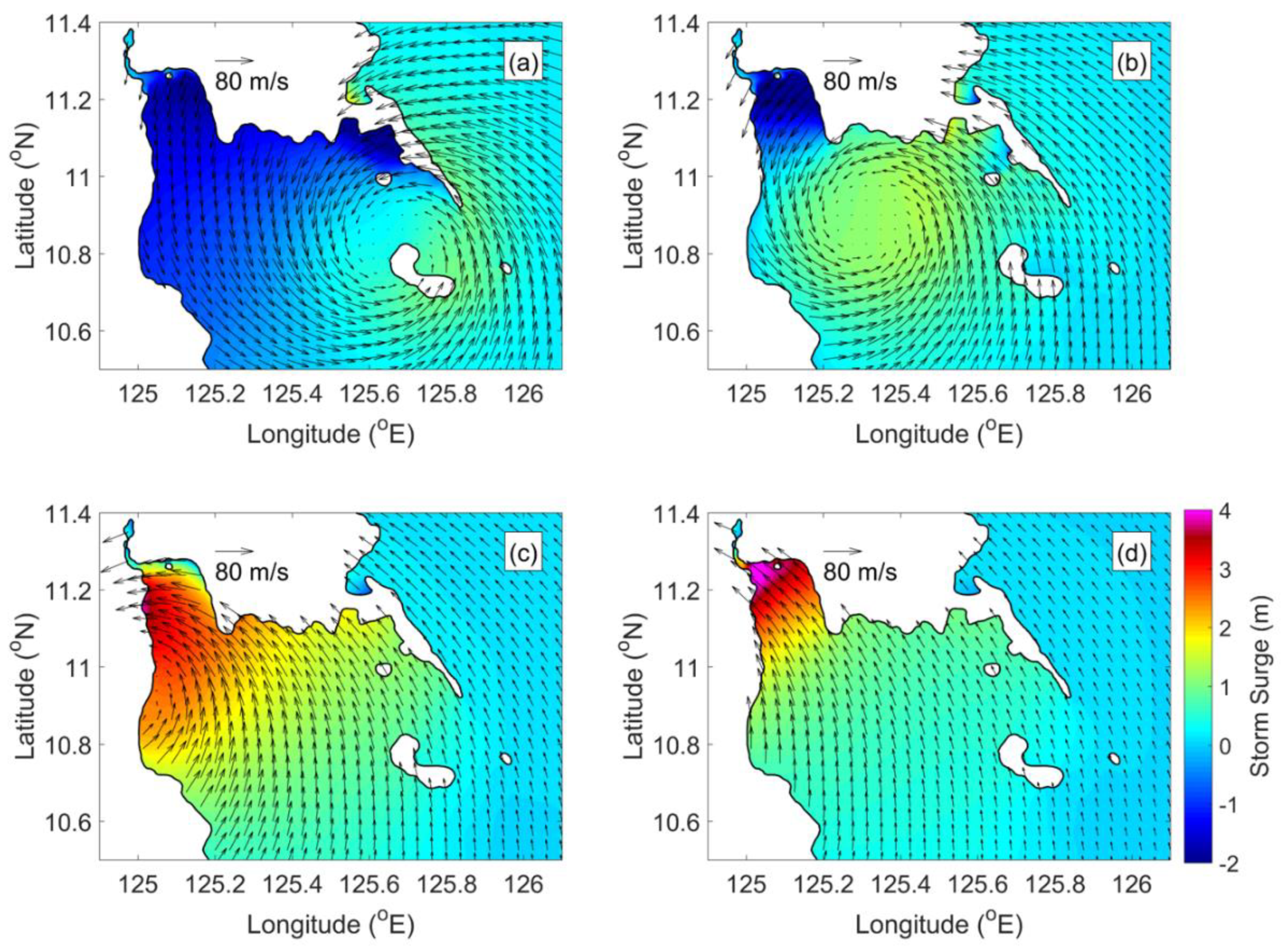
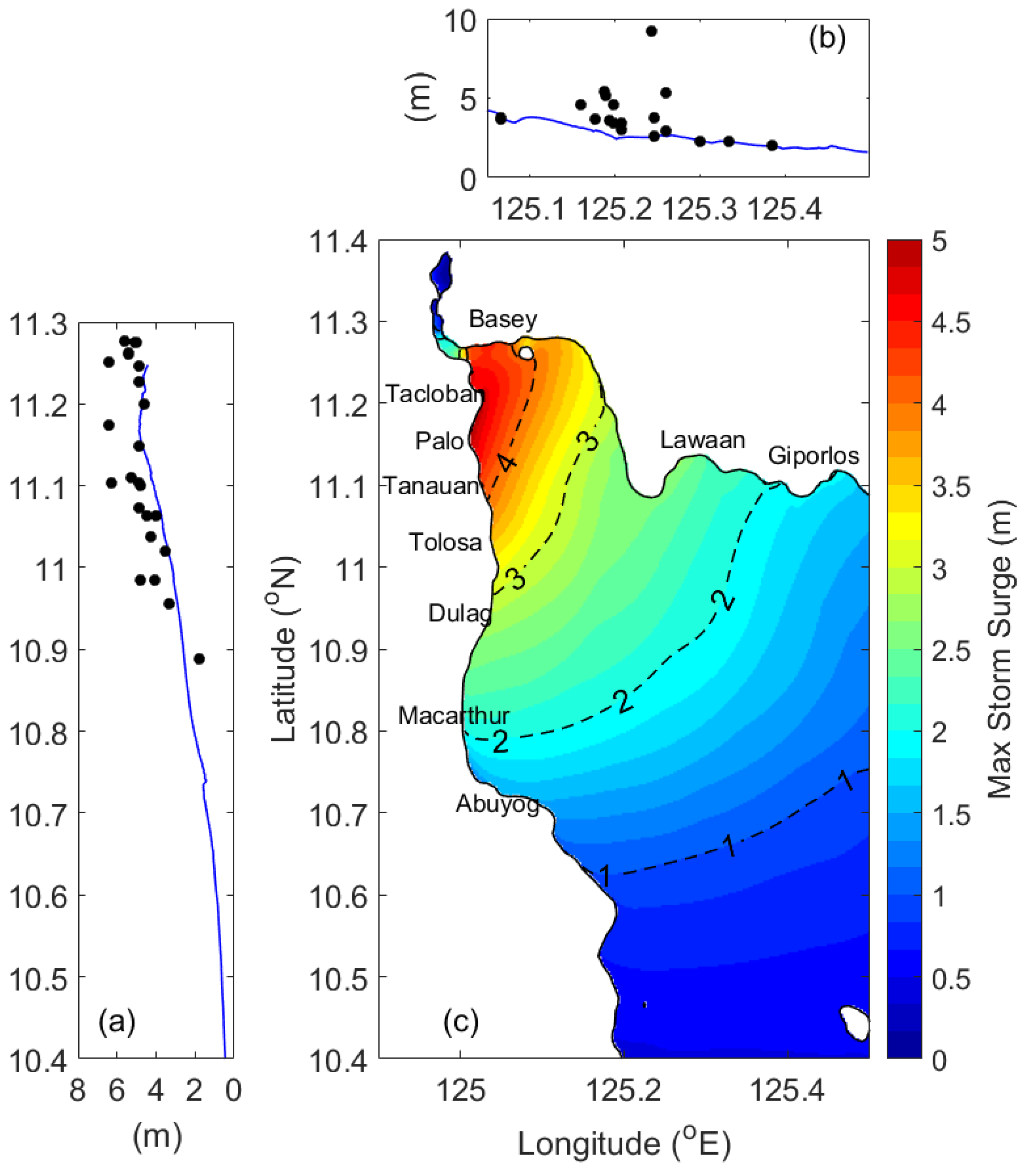
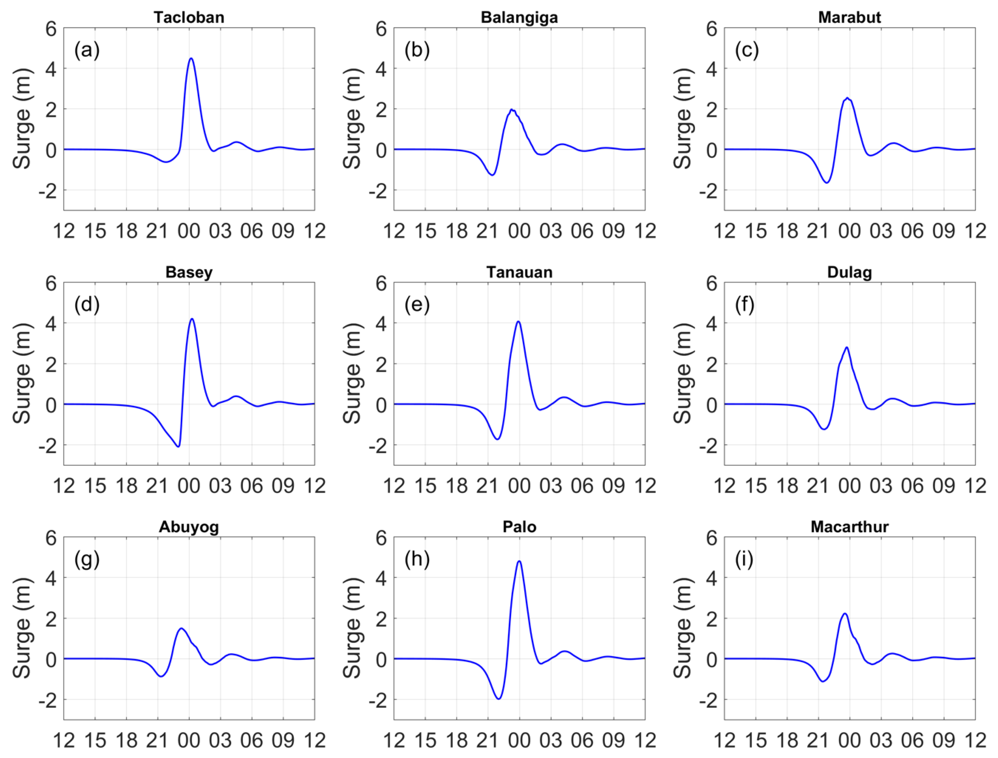
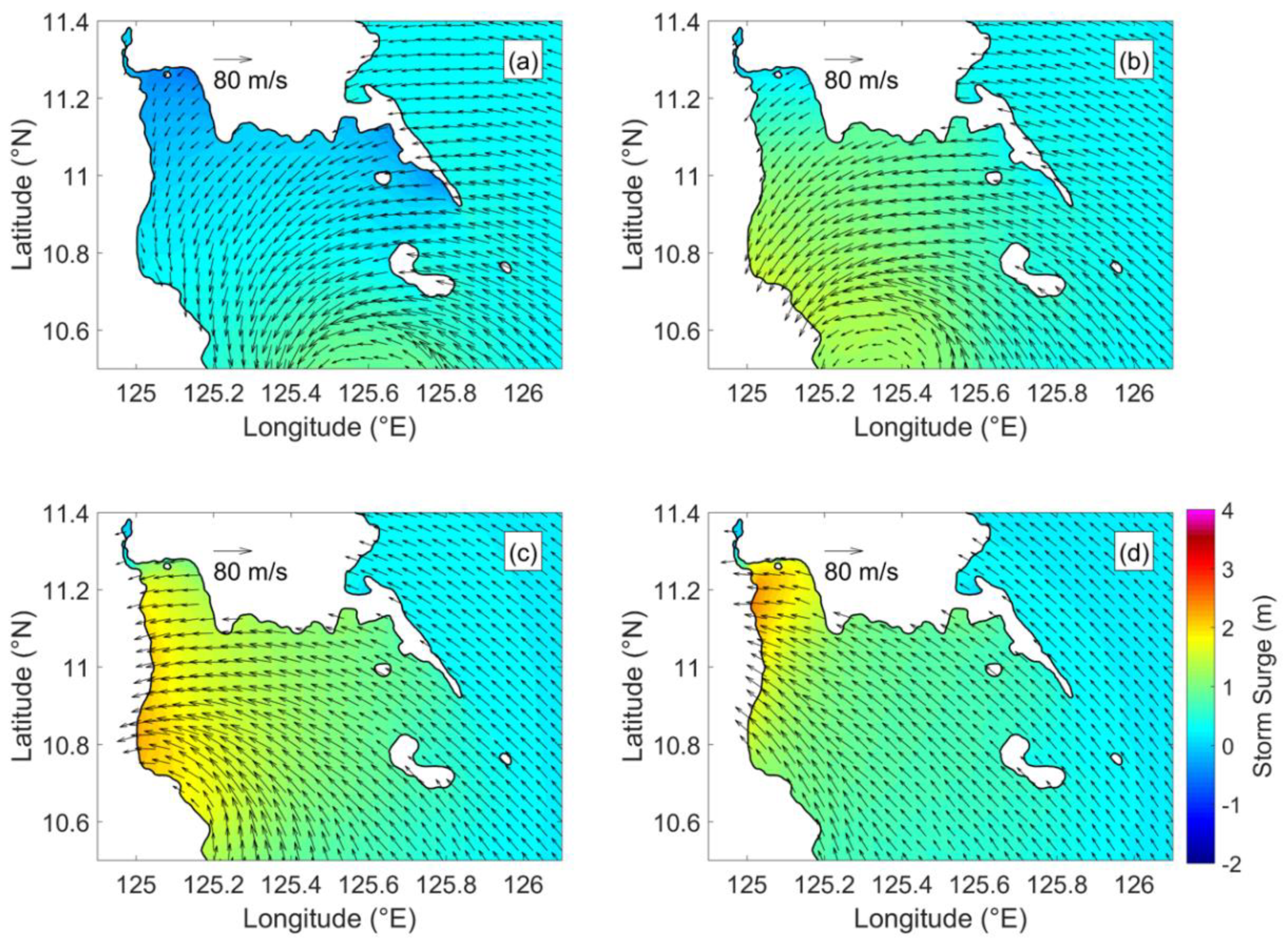
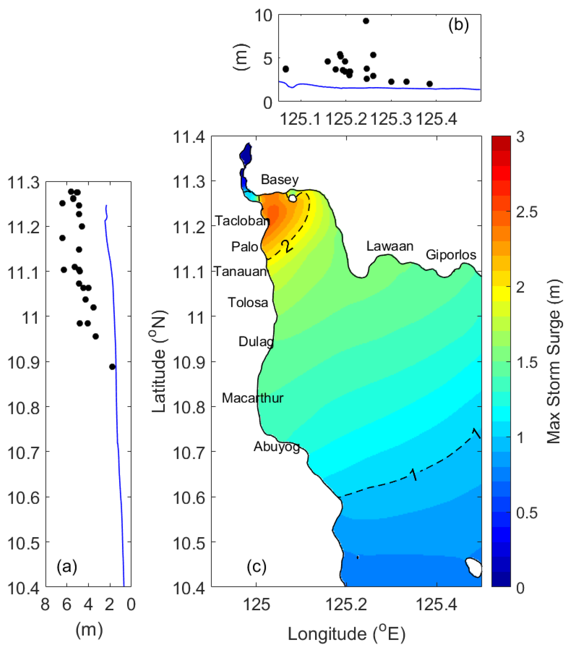
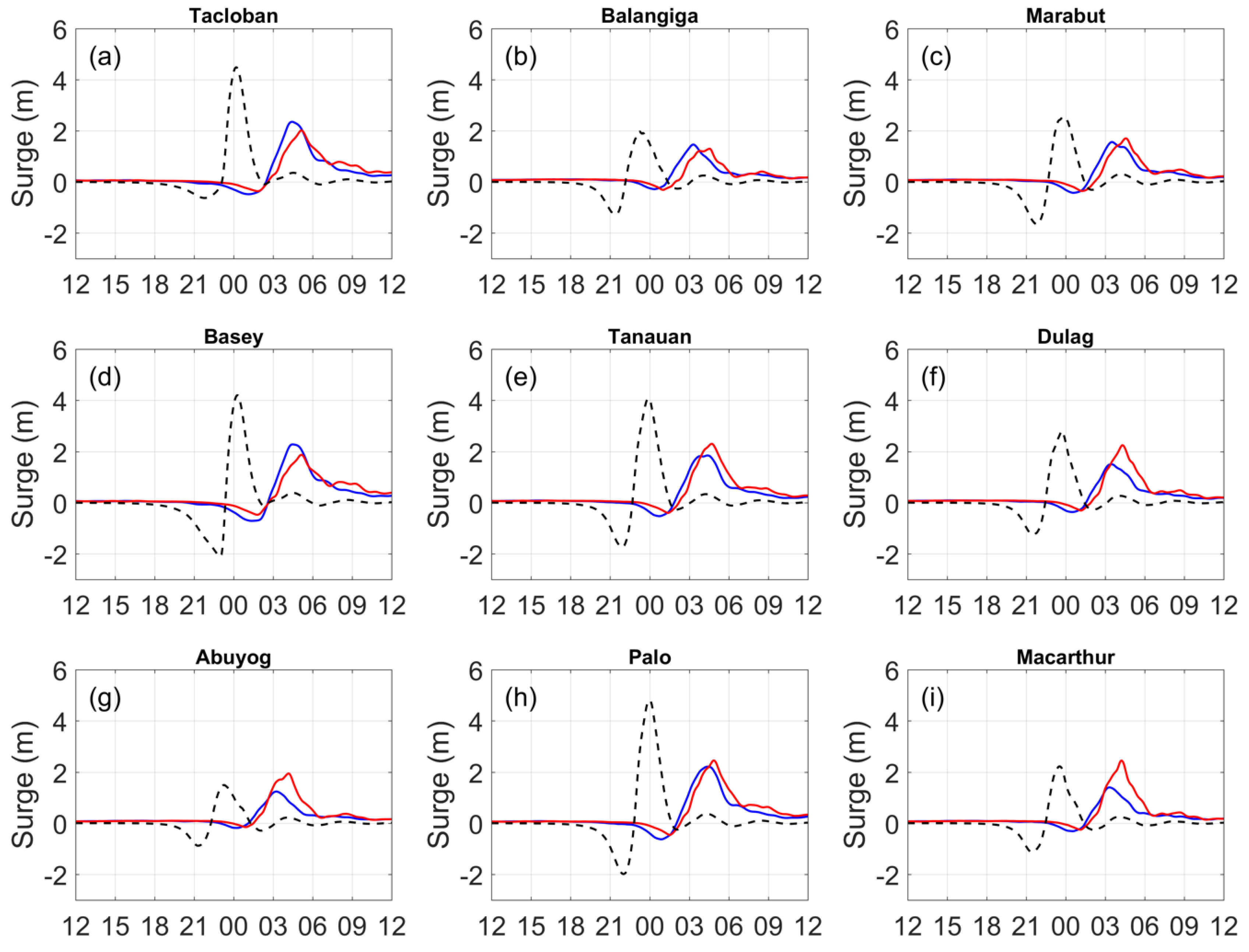
3.2. Haiyan’s Storm Surge Simulation by HWM

After examining the 10-m winds and sea-level pressures against the observation data at Guiuan weather station, the storm surge modeling driven by HWM are explored in this section.

In storm surge modeling, winds can amplify the surge heights in coastal regions when wind directions are more or less perpendicular to coasts. Besides, the intensity of winds is relative to the wind shear stresses over a water surface. Hence, before performing storm surge predictions, the wind fields on the standard level of 10 m shall be examined. In Figure 5, the snapshots of the 10-m winds predicted by HWM are presented. In Figure 5a, the storm center of Haiyan just enters the Leyte Gulf and passes over the small island in the south of the Samar Island. In a while, the value of 10-m winds blowing to the Samar Island is higher than 60 m/s, and the strong offshore winds occur in the San Pedro Bay. As shown in Figure 5b, Haiyan moves to the central regions of the Leyte Gulf, and the HWM-predicted winds hit the southern regions of the Samar Island, such as Giporlos and Balangiga. When Haiyan makes landfall at the Leyte Island, the severe onshore winds towards the San Pedro Bay can be found in Figure 5c. The winds of more than 60 m/s hit the regions in particular Tacloban, Basey, and Palo. After Haiyan makes landfall at Leyte Island, the southeastern winds keep blowing from the Leyte Gulf to the San Pedro Bay (see Figure 5d). As shown in Figure 5d, after the landfall, the cyclonic winds still maintain the wind speeds of more than 45 m/s.

In Figure 6, the computed storm surges driven by HWM are illustrated. Due to the strong offshore winds in the San Pedro Bay and the Leyte Gulf, the negative storm surges are generated accordingly (see Figure 6a,b). As shown in Figure 6c, when Haiyan makes landfall at the Leyte Island, the cyclonic winds push up the water hitting the regions such as Tacloban, Palo, and Tanauan. Storm surges of more than 3.5 m are observed in the simulation. After Haiyan makes landfall at the Leyte Island, the winds in the San Pedro Bay become southeastern (see Figure 6d). Because of these winds, the waters are piled up inside the bay and generate the significant storm surges of more than 4.0 m, which hit Tacloban, Palo, and Basey.

The maximum computed storm surges driven are shown in Figure 7, and the maximum computed surge heights along the coasts of the Leyte and Samar Islands are compared to the measured field survey data as well. In Figure 7a,b, the field survey data of Tajima et al. (2014) [33] with the Reliability A (clear mark and small error of survey) are presented and the tide effect has been removed. The profiles of maximum computed surge heights are acquired one grid away from the coasts to avoid the boundary effect. In Figure 7a,b, the simulation results agree well with the patterns of the measured water levels along the coasts of the Leyte Island and the Samar Island generally. Besides, relatively higher storm surges are found near the inner of the San Pedro Bay in both model results and the measured water levels. However, the measured water levels of more than 6 m can be found near the innermost part of the San Pedro Bay (see Figure 7a), where the wave overtopping and the up-wash of wind waves could be severe [19]. The model results may give an underestimation of water levels near the bay. Moreover, the comparisons are expected to be better if the inundation calculation can be performed with the detailed land elevation model and the shape of coastline in the Leyte Gulf and the San Pedro Bay [18]. As shown in Figure 7c, inside the San Pedro Bay, the maximum storm surges of more than 4.5 m are found in Basey, Tacloban, Palo, and Tanauan. These prominent maximum storm surges are attributed to the southeastern winds from the Leyte Gulf to the San Pedro Bay, making the water pile up inside the bay after Haiyan makes landfall at the Leyte Island (see Figure 6d).

In Figure 8, the time series of computed storm surges at numerical gauges are presented. In all stations, the records show the declines of the water-level first and then following quick rises within 3 h. This phenomenon corresponds to the witness reports about the “tsunami-like” wavefront hit Tacloban and Basey after the water-level receded [32,35]. Maximum storm surges of more than 4.0 m are found in Tacloban, Basey, Tanauan, and Palo (see Figure 8a,d,e,h), which corresponds to the maximum computed surges and field survey shown in Figure 7. There are two water-level measurements at Tacloban and Guiuan tidal stations during the passage of Haiyan [19]. The observation of the Tacloban tidal station was interrupted before the peak storm surge occurred; hence, this observation didn’t record the complete time series of water-level. In the Guiuan tide station which is located at the southeastern part of the Samar Island not the San Pedro Bay, the wind wave and storm surge interactions could be significant. Hence, we only use the field survey data of Tajima et al. (2014) [33] to compare the maximum computed storm surges as the model validation. More discussion on these observed water-levels can be found in Kumagai et al. (2016) [19] and Soria et al. (2016) [35].

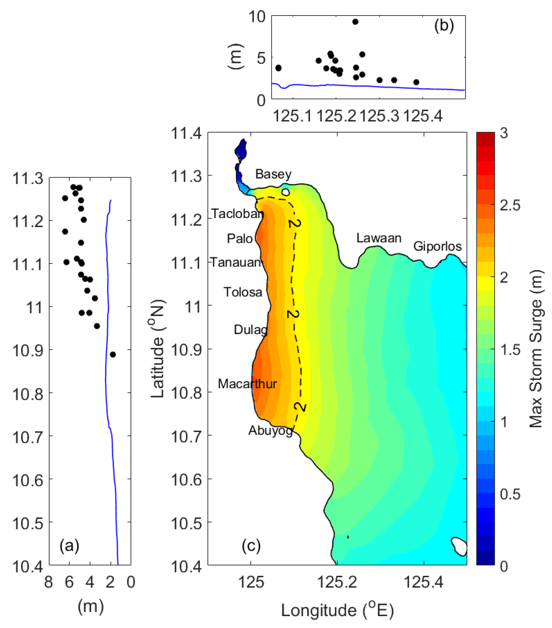
3.3. Haiyan’s Storm Surge Simulation by WRF-ARW

In this section, the results of storm surge modeling driven by WRF-ARW are explored. The 10-m winds and sea-level pressure from WRF-ARW 3 km and WRF-ARW 1 km with the 1-h time interval are used to drive the storm surge model. To reach the storm intensity of Haiyan in the WRF-ARW modeling, the nudging scheme, four-dimensional data assimilation (FDDA), is used from 00:00 UTC 4 November 2013 to 00:00 UTC 5 November 2013 (24 h). Afterward, the simulation is carried out by WRF-ARW only without the further use of data assimilation. Hence, the translation speed of Haiyan predicted by WRF-ARW is slower than the JMA best-track data (see Figure 9). As illustrated in Figure 9, the storm landfall locations between the JMA best-track and WRF-ARW 3 km are more or less the same and WRF-ARW 1 km predicted more south landfall location at the Leyte Island. The landfall times predicted by WRF-ARW 3 km and WRF-ARW 1 km at the Leyte Island are 4–5 h late than the best-track. The storm centers of WRF-ARW 3 km and WRF-ARW 1 km and their distance from the best-track are tabulated in

Table 3. The storm centers of WRF-ARW 3 km and WRF-ARW 1 km and their distances apart from those of the JMA best-track. The distance between the predicted storm center of WRF-ARW and that of the JMA best-track is calculated by the great-circle distance formula.

Date				WRF-ARW 3 km			WRF-ARW 1 km
Year	Month	Day	Hour	Longitude (° E)	Latitude (° N)	Distance (km)	Longitude (° E)	Latitude (° N)	Distance (km)
2013	11	7	00	133.22	9.02	58.38	133.40	8.73	66.48
2013	11	7	06	131.45	9.32	38.55	131.60	9.13	57.74
2013	11	7	12	129.63	9.72	78.60	130.04	9.46	132.22
2013	11	8	00	126.06	10.68	141.60	126.23	10.40	169.78
2013	11	8	06	124.15	11.22	180.81	124.36	10.85	211.54
2013	11	8	12	121.97	11.99	160.03	122.27	11.58	195.66

. More discussions about the WRF-ARW modeling can be found in Kueh et al. (2019) [15]. By the deviations of landfall locations and the translation speed of Haiyan from WRF-ARW, the results of storm surge prediction driven by WRF-ARW are anticipated to show different patterns from those driven by HWM.

In Figure 10 and Figure 11, the snapshots of 10-m winds of WRF-ARW 3 km and WRF-ARW 1 km are presented respectively. As shown in Figure 10a,b, the storm center of Haiyan predicted by WRF-ARW 3 km just arrives at the small island in the south of East Samar and then passes over it. The locations of the storm center are similar to the JMA’s best track (see Figure 6a). At these moments, the winds hit southeastern regions of the Samar Island and offshore winds occur in the San Pedro Bay. In Figure 10c, the storm center predicted by WRF-ARW 3 km tends to land near Mayorga, which is relatively south than the one predicted by HWM (see Figure 6c). After making landfall at the Leyte Island, the southeastern winds occur in the San Pedro Bay (see Figure 6d); however, the wind intensity is not as strong as HWM.

In Figure 11a, the storm center of Haiyan predicted by WRF-ARW 1 km passes over Dinagat islands, which is further south than the ones predicted by WRF-ARW 3 km and the JMA best track. Compared to wind speeds of WRF-ARW 3 km, WRF-ARW 1 km’s results are much more potent, about 20% stronger than that. As shown in Figure 11b, the winds of WRF-ARW 1 km are more parallel to the southern regions of the Samar Island. The wind speeds of more than 55 m/s are found in the east and northeast part to the storm center. WRF-ARW 1 km gives a further south landfall location than others; hence, the strong onshore winds hit the regions such as Macarthur, Dulag, and Tolosa (see Figure 11c). After making landfall at the Leyte Island, the southeastern winds blowing from the Leyte Gulf to the San Pedro Bay occur (see Figure 11d). Moreover, the stronger winds of WRF-ARW 1 km hit the regions such as Tolosa and Dulag and the maximum 10-m wind speed of more than 45 m/s is still found near the east coasts of the Leyte Island.

In the comparison between WRF-ARW 3 km and WRF-ARW 1 km, the significant discrepancy is the storm track, which affects the predicted landfall location at the Leyte Island and the southeastern winds blowing from the Leyte Gulf to the San Pedro Bay.

The computed storm surges driven by WRF-ARW 3 km and WRF-ARW 1 km are illustrated in Figure 12 and Figure 13, respectively. As shown in Figure 12a,b, due to the cyclonic winds, the negative storm surges occur in the Leyte Gulf and the San Pedro Bay. When the storm center of Haiyan approaches the Leyte Island, the positive storm surges of more than 1 m are generated (see Figure 12c). In Figure 12d, after Haiyan makes landfall at the Leyte Island, the storm surges of more than 2.0 m pile up in the San Pedro Bay and hit Tacloban, Palo, and Tanauan. The pattern of computed storm surges is similar to that predicted by HWM (see Figure 6d) but lower. In the results driven by WRF-ARW 1 km, because of the more south predicted storm track, the storm surges of more than 2.0 m first hit Dulag and Macarthur (see Figure 13b,c). After Haiyan makes landfall at the Leyte Island, the storm surges of more than 2.0 m occur in the San Pedro Bay (see Figure 13d).

In Figure 14 and Figure 15, the maximum computed storm surges driven by WRF-ARW 3 km and WRF-ARW 1 km are illustrated and the maximum computed surge heights along the coasts of the Leyte Island and the Samar Island are compared to the measured field survey data [33]. In Figure 14c, the maximum storm surges of more than 2 m driven by WRF-ARW 3 km are found in Tacloban, Palo, Tanauan, and Basey, which of them are inside the San Pedro Bay. The pattern is similar to the one driven by HWM; however, the amplitude of maximum computed storm surges inside the San Pedro Bay is almost twice lower. Since lower maximum computed storm surges are predicted, the results cannot match perfectly with the field survey data (see Figure 14a,b). In the result driven by WRF-ARW 1 km, the prominent computed maximum storm surges of more than 2 m are also found on the east coast of Leyte Island such as Dulag, Macarthur, and Abuyog (see Figure 15b). As expected, the results cannot match well with the field survey data as well (see Figure 15a,c).

In Figure 16, the time series of computed storm surges in the numerical gauges are shown. Since both of WRF-ARW 3 km and WRF-ARW 1 km predict slower storm forward motion than the best track, the arrival time of peak storm surges occur behind those in the HWM’s results. In the stations in the inner of the San Pedro Bay such as Tacloban and Basey, the results driven by WRF-ARW 3 km and WRF-ARW 1 km have the similar patterns. In these stations, the peak predicted storm surges driven by WRF-ARW 3 km are slightly higher than those by WRF-ARW 1 km; however, both of them are still lower than those driven by HWM. For stations such as Abuyog, Macarthur, and Dulag, because WRF-ARW 1 km predicts the further south landfall location at the Leyte Island, the winds blow toward these regions and cause storm surges about 0.8–1.0 m higher than those in WRF-ARW 3 km. Moreover, in these stations, the differences of maximum storm surges driven between HWM and WRF-ARW are not as prominent as those located in the San Pedro Bay.

Storm surge modeling driven by both WRF-ARW 3 km and WRF-ARW 1 km cannot reproduce obvious storm surges in the San Pedro Bay. For WRF-ARW 3 km, the predicted storm track is close to the JMA’s best track; however, WRF-ARW 3 km underestimates the wind intensity. Despite WRF-ARW 1 km gives comparable higher wind intensity, it predicts relatively south storm track of Haiyan, which makes the underestimation of storm surges in the San Pedro Bay. Moreover, both of WRF-ARW 3 km and WRF-ARW 1 km predict slower storm forward motion, which also affects the storm surge calculation. Next, the effects of the storm track and the storm forward speed on generating storm surges in the San Pedro Bay and the Leyte Gulf will be explored.

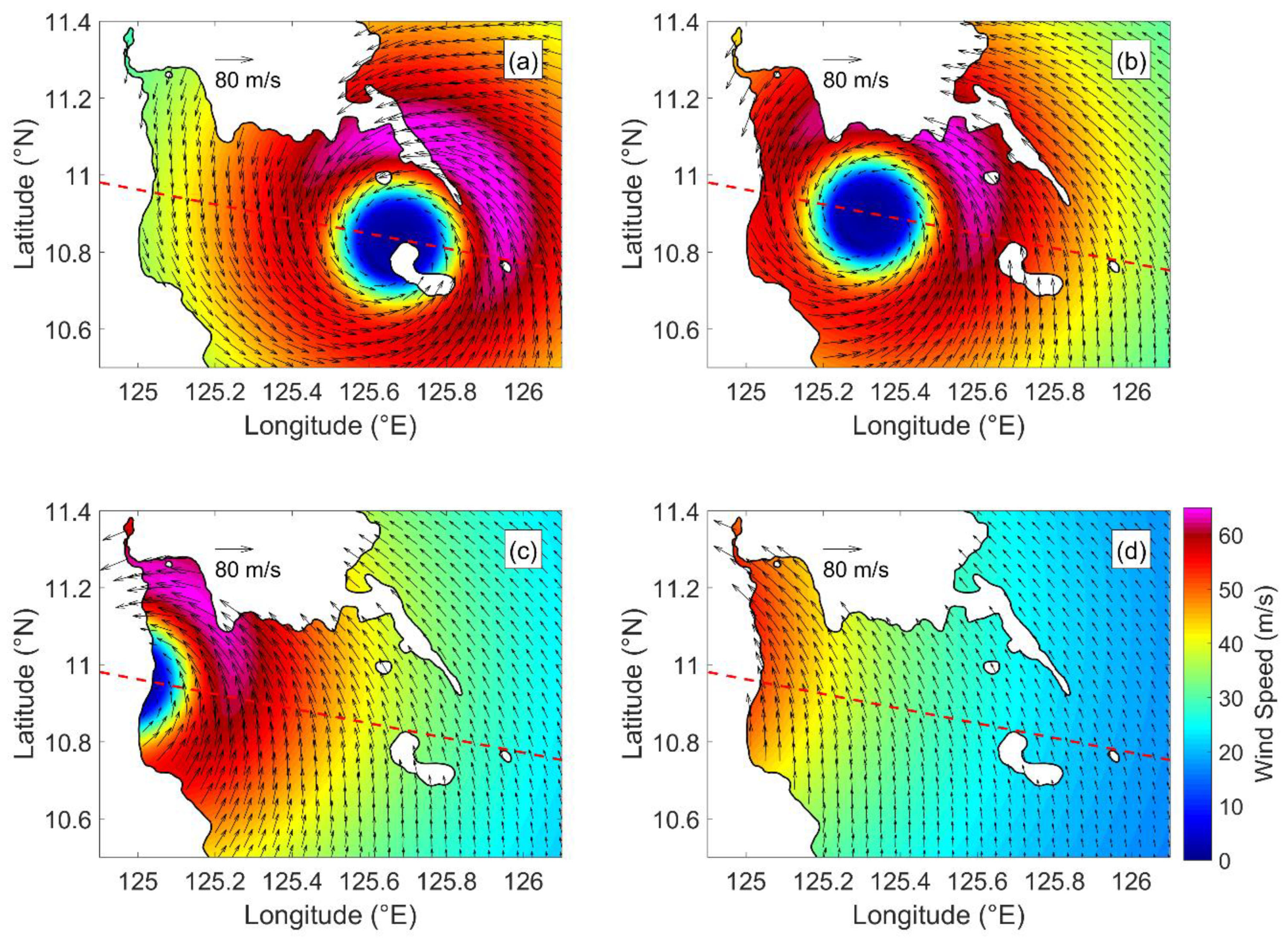
3.4. Experiment for Storm Forward Speed

In previous sections, the storm surge modeling driven by HWM, WRF-ARW 3 km, and WRF-ARW 1 km presents the prominent differences due to the deviations of predicted storm tracks and the forward speed of storm. Tajima et al. (2016) [38] and Kumagai et al. (2016) [19] have conducted a series of sensitivity analysis on the variations of storm track and the storm forward speed to the storm surges in the San Pedro Bay. Tajima et al. (2016) [38] found that Haiyan’s storm track seems to be the worse one for the regions near Palo and Tanauan. Besides, they pointed out that maximum storm surge at Tacloban will be reduced by about 45% if the forward speed of Haiyan is decreased by 50%. Kumagai et al. (2016) [19] indicated that the storm surges near Dulag will increase if Haiyan’s storm track become more south, but storm surges in the San Pedro Bay will reduce. Both of these studies correspond to our findings in the storm surge modeling driven by HWM, WRF-ARW 3 km, and WRF-ARW 1 km.

In this section, the numerical experiment focused on a storm forward speed is carried out since only few stations have been explored [38] and a constant forward speed was assumed [19]. Because Haiyan’s storm surge simulation affected by the storm-track variations [19,38] and the radius of maximum winds have been explored carefully [18], these discussions will not be included here. In this numerical experiment, besides the original storm forward speed, this study includes two comparable cases: forward speed increased by 10% and decreased by 10%. The 10-m winds and the sea-level pressures in this experiment are from HWM. To analyze the hydrodynamical response of storm surges to a storm forward speed, the wind asymmetry modified by a storm forward motion is considered by the original forward speed for the sake of simplicity.

The time series of storm surges in the numerical gauges are illustrated in Figure 17. In the stations located inside the San Pedro Bay such as Tacloban, Basey, Palo, and Tanauan, the maximum computed storm surges are intensified by a faster storm forward speed (see Figure 17a,d,e,h). On the other hand, by considering the slower storm forward speed, the maximum computed storm surges are reduced. However, in the stations outside the San Pedro Bay such as Balangiga and Abuyog, the maximum computed storm surges are reduced in the case with the faster storm forward speed (see Figure 17b,g). The statistical results of the maximum computed storm surges are tabulated in

Table 4. Maximum computed storm surges in the numerical experiment using original, faster, slower storm forward speed.

Station Name	${\mathit{\eta }}_{\mathit{m}\mathit{a}\mathit{x}}$ (m)	Faster Storm Forward Motion (10% Increased)		Slower Storm Forward Motion (10% Decreased)
		${\mathit{\eta }}_{\mathit{m}\mathit{a}\mathit{x}\mathbf{,}\mathit{f}}$ (m)	$\mathbf{\left(}{\mathit{\eta }}_{\mathit{m}\mathit{a}\mathit{x}\mathbf{,}\mathit{f}}\mathbf{/}{\mathit{\eta }}_{\mathit{m}\mathit{a}\mathit{x}}\mathbf{\right)}\mathbf{-}\mathbf{1}$	${\mathit{\eta }}_{\mathit{m}\mathit{a}\mathit{x}\mathbf{,}\mathit{s}}$ (m)	$\mathbf{\left(}{\mathit{\eta }}_{\mathit{m}\mathit{a}\mathit{x}\mathbf{,}\mathit{s}}\mathbf{/}{\mathit{\eta }}_{\mathit{m}\mathit{a}\mathit{x}}\mathbf{\right)}\mathbf{-}\mathbf{1}$
Tacloban	4.487	4.701	4.77%	4.259	−5.08%
Balangiga	1.985	1.870	−5.79%	2.030	2.27%
Marabut	2.55	2.644	3.69%	2.387	−6.39%
Basey	4.202	4.498	7.04%	3.914	−6.85%
Tanauan	4.069	4.264	4.79%	3.840	−5.63%
Dulag	2.798	2.865	2.39%	2.652	−5.22%
Abuyog	1.495	1.407	−5.89%	1.534	2.61%
Palo	4.804	5.039	4.89%	4.547	−5.35%
Macarthur	2.225	2.164	−2.74%	2.208	−0.76%

. From Table 4, considering the storm forward speed increased by 10%, the extreme values of storm surges in the stations inside the San Pedro Bay such as Tacloban and Tanauan are intensified by 4.5–7.0%; however, the reductions of 5.3–6.8% on the maximum values are shown when considering the slower forward speed.

4. Conclusions

This study has explored the discrepancies of the storm surge predictions driven by a parametric wind (PW) model and a numerical weather prediction (NWP) model. By shedding light upon the discrepancies, the storm surges of 2013 Typhoon Haiyan in the Leyte Gulf and the San Pedro Bay have been studied. The frictional-free, steady-state, and geostrophic-balancing solutions on the storm winds and sea-level pressures given by the Holland wind model (HWM) have been first verified against the observed data at the Guiuan weather station. The 10-m winds predicted by WRF-ARW (Weather Research and Forecasting-Advanced Research WRF), which solves the 3D time-integrated, compressible, and non-hydrostatic Euler equations, have been compared with the ones by HWM. In the results of computed storm surges driven by HWM, the storm surges of more than 4.5 m have been found in the San Pedro Bay due to the water piling up and the pattern is agreed well with the field survey data. However, in the results by both WRF-ARW 3 km and WRF-ARW 1 km, the maximum storm surge in the San Pedro Bay is almost half than that driven by HWM. The significant differences among HWM, WRF-ARW 3 km, and WRF-ARW 1 km are caused by the predicted landfall location of Haiyan, the storm intensity, and the storm forward speed. The numerical experiment focused on the storm forward speed has pointed out that the extreme values of storm surges inside the San Pedro Bay can be intensified by 4.5–7.0% when the storm forward speed is increased by 10%. This study hopes to pave the way for future research in understanding the discrepancies in predicting storm surges driven by either of the PW or NWP models and thus benefiting storm surge predictions in a semi-enclosed bay.

References

1. Fritz, H.M.; Blount, C.; Sokoloski, R.; Singleton, J.; Fuggle, A.; McAdoo, B.G.; Moore, A.; Grass, C.; Tate, B. Hurricane Katrina Storm Surge Distribution and Field Observations on the Mississippi Barrier Islands. Estuar. Coast. Shelf Sci. 2007, 74, 12–20. [Google Scholar] [CrossRef]
2. Zhang, W.Z.; Shi, F.; Hong, H.S.; Shang, S.P.; Kirby, J.T. Tide-Surge Interaction Intensified by the Taiwan Strait. J. Geophys. Res. 2010, 115. [Google Scholar] [CrossRef] [Green Version]
3. Tang, Y.M.; Sanderson, B.; Holland, G.J.; Grimshaw, R. A Numerical Study of Storm Surges and Tides, with Application to the North Queensland Coast. J. Phys. Oceanogr. 1996, 26, 2700–2711. [Google Scholar] [CrossRef] [Green Version]
4. Mastenbroek, C.; Burgers, G.; Janssen, P. The Dynamical Coupling of a Wave Model and a Storm Surge Model through the Atmospheric Boundary Layer. J. Phys. Oceanogr. 1993, 23, 1856–1866. [Google Scholar] [CrossRef] [Green Version]
5. Bunya, S.; Dietrich, J.C.; Westerink, J.J.; Ebersole, B.A.; Smith, J.M.; Atkinson, J.H.; Jensen, R.; Resio, D.T.; Luettich, R.A.; Dawson, C.; et al. A High-Resolution Coupled Riverine Flow, Tide, Wind, Wind Wave, and Storm Surge Model for Southern Louisiana and Mississippi. Part I: Model Development and Validation. Mon. Weather Rev. 2010, 138, 345–377. [Google Scholar] [CrossRef] [Green Version]
6. Dietrich, J.C.; Bunya, S.; Westerink, J.J.; Ebersole, B.A.; Smith, J.M.; Atkinson, J.H.; Jensen, R. A High-Resolution Coupled Riverine Flow, Tide, Wind, Wind Wave, and Storm Surge Model for Southern Louisiana and Mississippi. Part II: Synoptic Description and Analysis of Hurricanes Katrina and Rita. Mon. Weather Rev. 2010, 138, 378–404. [Google Scholar] [CrossRef] [Green Version]
7. Schiermeier, Q. Did Climate Change Cause Typhoon Haiyan? Nature 2013. [Google Scholar] [CrossRef]
8. Elsner, J.B.; Kossin, J.P.; Jagger, T.H. The Increasing Intensity of the Strongest Tropical Cyclones. Nature 2008, 455, 92–95. [Google Scholar] [CrossRef]
9. Zhong, L.; Li, M.; Zhang, D.L. How do uncertainties in hurricane model forecasts affect storm surge predictions in a semi-enclosed bay? Estuar. Coast. Shelf Sci. 2010, 90, 61–72. [Google Scholar] [CrossRef]
10. Skamarock, W.C.; Klemp, J.B.; Dudhia, J.; Gill, D.O.; Barker, D.M.; Duda, M.G.; Huang, X.Y.; Wang, W.; Powers, J.G. A description of the advanced research WRF version 3. NCAR Tech. 2008, 113. [Google Scholar] [CrossRef]
11. Tsuboki, K.; Sakakibara, A. Large-scale parallel computing of cloud resolving storm simulator. In International Symposium on High Performance Computing; Springer: Berlin/Heidelberg, Germany, 2002; pp. 243–259. [Google Scholar]
12. Dee, D.P.; Uppala, S.M.; Simmons, A.J.; Berrisford, P.; Poli, P.; Kobayashi, S.; Andrae, U.; Balmaseda, M.A.; Balsamo, G.; Bauer, D.P.; et al. The ERA-Interim reanalysis: Configuration and performance of the data assimilation system. Q. J. R. Meteorol. Soc. 2011, 137, 553–597. [Google Scholar] [CrossRef]
13. Mori, N.; Kato, M.; Kim, S.; Mase, H.; Shibutani, Y.; Takemi, T.; Tsuboki, K.; Yasuda, T. Local Amplification of Storm Surge by Super Typhoon Haiyan in Leyte Gulf. Geophys. Res. Lett. 2014, 41, 5106–5113. [Google Scholar] [CrossRef] [PubMed] [Green Version]
14. Li, F.; Song, J.; Xia, L. A preliminary evaluation of the necessity of using a cumulus parameterization scheme in high-resolution simulations of Typhoon Haiyan (2013). Natl. Hazards 2018, 92, 647–671. [Google Scholar] [CrossRef]
15. Kueh, M.T.; Chen, W.M.; Sheng, Y.F.; Lin, S.C.; Wu, T.R.; Yen, E.; Tsai, Y.L.; Lin, C.Y. Effects of horizontal resolution and air-sea flux parameterization on the intensity and structure of simulated Typhoon Haiyan (2013). Natl. Hazards Earth Syst. Sci. 2018, 19, 1509–1539. [Google Scholar] [CrossRef] [Green Version]
16. Jelesnianski, C.; Chen, J.; Shaffer, W.; Gilad, A. A Hurricane Storm Surge Forecast Model. In Proceedings of the SLOSH, Washington, DC, USA, 10–12 September 1984. [Google Scholar] [CrossRef]
17. Wu, T.R.; Tsai, Y.L.; Terng, C.T. The Recent Development of Storm Surge Modeling in Taiwan. Proc. IUTAM 2017, 25, 70–73. [Google Scholar] [CrossRef]
18. Kim, S.; Mori, N.; Mase, H.; Yasuda, T. The Role of Sea Surface Drag in a Coupled Surge and Wave Model for Typhoon Haiyan 2013. Ocean Model. 2015, 96, 65–84. [Google Scholar] [CrossRef]
19. Kumagai, K.; Mori, N.; Nakajo, S. Storm Surge Hindcast and Return Period of a Haiyan-Like Super Typhoon. Coast. Eng. J. 2016, 58, 1640001-1–1640001-24. [Google Scholar] [CrossRef]
20. Li, N.; Roeber, V.; Yamazaki, Y.; Heitmann, T.W.; Bai, Y.; Cheung, K.F. Integration of Coastal Inundation Modeling from Storm Tides to Individual Waves. Ocean. Model. 2014, 83, 26–42. [Google Scholar] [CrossRef]
21. Li, N.; Yamazaki, Y.; Roeber, V.; Cheung, K.F.; Chock, G. Probabilistic Mapping of Storm-Induced Coastal Inundation for Climate Change Adaptation. Coast. Eng. 2018, 133, 126–141. [Google Scholar] [CrossRef]
22. Jeong, C.K.; Panchang, V.; Demirbilek, Z. Parametric adjustments to the rankine vortex wind model for Gulf of Mexico hurricanes. J. Offshore Mech. Arct. Eng. 2012, 134, 041102. [Google Scholar] [CrossRef]
23. Jelesnianski, C.P. Slosh: Sea, Lake and Overland Surges from Hurricanes; US Department of Commerce, National Oceanic and Atmospheric Administration, National Weather Service: Silver Spring, MD, USA, 1992; Volume 48.
24. Holland, G.J. An Analytic Model of the Wind and Pressure Profiles in Hurricanes. Mon. Weather Rev. 1980, 108, 1212–1218. [Google Scholar] [CrossRef]
25. Xie, L.; Bao, S.; Pietrafesa, L.J.; Foley, K.; Fuentes, M. A Real-Time Hurricane Surface Wind Forecasting Model: Formulation and Verification. Mon. Weather Rev. 2006, 134, 1355–1370. [Google Scholar] [CrossRef]
26. Holland, G.J.; Belanger, J.I.; Fritz, A. A Revised Model for Radial Profiles of Hurricane Winds. Mon. Weather Rev. 2010, 138, 4393–4401. [Google Scholar] [CrossRef]
27. Lin, N.; Chavas, D. On hurricane parametric wind and applications in storm surge modeling. J. Geophys. Res. Atmos. 2012, 117, D9. [Google Scholar] [CrossRef]
28. Liu, F.; Sasaki, J. Hybrid methods combining atmospheric reanalysis data and a parametric typhoon model to hindcast storm surges in Tokyo Bay. Sci. Rep. 2019, 9, 1–10. [Google Scholar] [CrossRef] [PubMed]
29. Hsiao, S.C.; Chen, H.; Wu, H.L.; Chen, W.B.; Chang, C.H.; Guo, W.D.; Chen, Y.M.; Lin, L.Y. Numerical Simulation of Large Wave Heights from Super Typhoon Nepartak (2016) in the Eastern Waters of Taiwan. J. Mar. Sci. Eng. 2020, 8, 217. [Google Scholar] [CrossRef] [Green Version]
30. Cheung, K.F.; Phadke, A.C.; Wei, Y.; Rojas, R.; Douyere, Y.M.; Martino, C.D.; Houstan, S.H.; Liao, S. Modeling of storm-induced coastal flooding for emergency management. Ocean. Eng. 2003, 30, 1353–1386. [Google Scholar] [CrossRef]
31. NDRRMC. Effects of Typhoon “YOLANDA” (HAIYAN) Technical Report; National Disaster Risk Reduction and Management Council: Quezon City, Philippines, 2014.
32. Takagi, H.; Esteban, M.; Shibayama, T.; Mikami, T.; Matsumaru, R.; de Leon, M.; Nakamura, R. Track analysis, simulation, and field survey of the 2013 Typhoon Haiyan storm surge. J. Flood Risk Manag. 2017, 10, 42–52. [Google Scholar] [CrossRef]
33. Tajima, Y.; Yasuda, T.; Pacheco, B.M.; Cruz, E.C.; Kawasaki, K.; Nobuoka, H.; Aquino, R. Initial report of JSCE-PICE joint survey on the storm surge disaster caused by Typhoon Haiyan. Coast. Eng. J. 2014, 56, 1450006. [Google Scholar] [CrossRef]
34. Mas, E.; Bricker, J.; Kure, S.; Adriano, B.; Yi, C.; Suppasri, A.; Koshimura, S. Field survey report and satellite image interpretation of the 2013 Super Typhoon Haiyan in the Philippines. Natl. Hazards Earth Syst. Sci. 2015, 15. [Google Scholar] [CrossRef] [Green Version]
35. Soria, J.L.A.; Switzer, A.D.; Villanoy, C.L.; Fritz, H.M.; Hope, P.; Bilgera, T.; Cabrera, O.C.; Siringan, F.P.; Maria, Y.T.S.; Ramos, R.D.; et al. Repeat Storm Surge Disasters of Typhoon Haiyan and Its 1897 Predecessor in the Philippines. Bull. Am. Meteorol. Soc. 2016, 97, 31–48. [Google Scholar] [CrossRef]
36. Mikami, T.; Shibayama, T.; Takagi, H.; Matsumaru, R.; Esteban, M.; Thao, N.D.; Kumagaim, K. Storm surge heights and damage caused by the 2013 Typhoon Haiyan along the Leyte Gulf coast. Coast. Eng. J. 2016, 58, 1640005. [Google Scholar] [CrossRef]
37. Takayabu, I.; Hibino, K.; Sasaki, H.; Shiogama, H.; Mori, N.; Shibutani, Y.; Takemi, T. Climate change effects on the worst-case storm surge: A case study of Typhoon Haiyan. Environ. Res. Lett. 2015, 10, 064011. [Google Scholar] [CrossRef]
38. Tajima, Y.; Gunasekara, K.H.; Shimozono, T.; Cruz, E.C. Study on locally varying inundation characteristics induced by super Typhoon Haiyan. Part 1: Dynamic behavior of storm surge and waves around San Pedro Bay. Coast. Eng. J. 2016, 58, 1640002. [Google Scholar] [CrossRef] [Green Version]
39. Szydłowski, M.; Kolerski, T.; Zima, P. Impact of the Artificial Strait in the Vistula Spit on the Hydrodynamics of the Vistula Lagoon (Baltic Sea). Water 2019, 11, 990. [Google Scholar] [CrossRef] [Green Version]
40. Dean, R.G.; Dalrymple, R.A. Water Wave Mechanics for Engineers and Scientists; World Scientific Publishing Company: Singapore, 1991; Volume 2. [Google Scholar]
41. Liang, S.-J.; Young, C.C.; Dai, C.; Wu, N.J.; Hsu, T.W. Simulation of Ocean Circulation of Dongsha Water Using Non-Hydrostatic Shallow-Water Model. Water 2016, 12, 2832. [Google Scholar] [CrossRef]
42. Lapidez, J.P.; Tablazon, J.; Dasallas, L.; Gonzalo, L.A.; Cabacaba, K.M.; Ramos, M.M.A.; Suarez, J.K.; Santiago, J.; Lagmay, A.M.F.; Malano, V. Identification of storm surge vulnerable areas in the Philippines through the simulation of Typhoon Haiyan-induced storm surge levels over historical storm tracks. Natl. Hazards Earth Syst. Sci. 2015, 3. [Google Scholar] [CrossRef] [Green Version]
43. Lagmay, A.M.F.; Agaton, R.P.; Bahala, M.A.C.; Briones, J.B.L.T.; Cabacaba, K.M.C.; Caro, C.V.C.; Dasallas, L.L.; Gonalo, L.A.L.; Ladiero, C.N.; Lapidez, J.P.; et al. Devastating storm surges of Typhoon Haiyan. Int. J. Dis. Risk Reduct. 2015, 11, 1–12. [Google Scholar] [CrossRef]
44. Liu, P.L.F.; Cho, Y.S.; Briggs, M.J.; Kanoglu, U.; Synolakis, C.E. Runup of solitary waves on a circular island. J. Fluid Mech. 1995, 302, 259–285. [Google Scholar] [CrossRef]
45. Liu, P.L.F.; Cho, Y.S.; Yoon, S.B.; Seo, S.N. Numerical simulations of the 1960 Chilean tsunami propagation and inundation at Hilo, Hawaii. In Tsunami: Progress in Prediction, Disaster Prevention and Warning; Springer: Dordrecht, The Netherlands, 1995; pp. 99–115. [Google Scholar]
46. Wang, X.; Liu, P.L.F. An analysis of 2004 Sumatra earthquake fault plane mechanisms and Indian Ocean tsunami. J. Hydraul. Res. 2006, 44, 147–154. [Google Scholar] [CrossRef]
47. Li, L.; Qiu, Q.; Huang, Z. Numerical modeling of the morphological change in Lhok Nga, west Banda Aceh, during the 2004 Indian Ocean tsunami: Understanding tsunami deposits using a forward modeling method. Natl. Hazards 2012, 64, 1549–1574. [Google Scholar] [CrossRef]
48. Lin, S.C.; Wu, T.R.; Yen, E.; Chen, H.Y.; Hsu, J.; Tsai, Y.L.; Philip, L.F. Development of a tsunami early warning system for the South China Sea. Ocean. Eng. 2015, 100, 1–18. [Google Scholar] [CrossRef]
49. Takagi, H.; Li, S.; Leon, M.; Esteban, M.; Mikami, T.; Matsumaru, R.; Shibayama, T.; Nakamura, R. Storm surge and evacuation in urban areas during the peak of a storm. Coast. Eng. 2016, 108, 1–9. [Google Scholar] [CrossRef] [Green Version]
50. Garzon, J.L.; Ferreira, C.M. Storm surge modeling in large estuaries: Sensitivity analyses to parameters and physical processes in the Chesapeake Bay. J. Marine Sci. Eng. 2016, 4, 45. [Google Scholar] [CrossRef] [Green Version]
51. Graham, L.; Butler, T.; Walsh, S.; Dawson, C.; Westerink, J.J. A measure-theoretic algorithm for estimating bottom friction in a coastal inlet: Case study of bay st. Louis during hurricane Gustav (2008). Mon. Weather Rev. 2017, 145, 929–954. [Google Scholar] [CrossRef]
52. Wu, J. Wind-stress coefficients over sea surface from breeze to hurricane. J. Geophys. Res. Oceans 1982, 87, 9704–9706. [Google Scholar] [CrossRef]
53. Liu, P.L.F.; Woo, S.B.; Cho, Y.S. Computer Programs for Tsunami Propagation and Inundation; Technical Report; Cornell University: New York, NY, USA, 1998. [Google Scholar]
54. Tsai, Y.L. The Development of Storm Surge Fast Calculation System and the Reconstruction of 1845 Yunlin Kouhu Event. Master’s Thesis, National Central University, Taoyuan, Taiwan, 2014. [Google Scholar]
55. Arakawa, A.; Lamb, V.R. Computational design of the basic dynamical processes of the UCLA general circulation model. Gen. Circ. Models Atmos. 1977, 17, 173–265. [Google Scholar]
56. Kim, S.Y.; Mori, N.; Shibutani, Y.; Yasuda, T.; Mase, H. Hindcast of storm surges and waves caused by Typhoon Haiyan using a coupling model of surge and wave. J. JSCE B2 Coast. Eng. 2014, 70, I_226–I_230. [Google Scholar]
57. Phadke, A.C.; Martino, C.D.; Cheung, K.F.; Houston, S.H. Modeling of tropical cyclone winds and waves for emergency management. Ocean. Eng. 2003, 30, 553–578. [Google Scholar] [CrossRef]
58. Schloemer, R.W. Analysis and Synthesis of Hurricane Wind Patterns over Lake Okeechobee; US Department of Commerce Weather Bureau: Miami, FL, USA, 1954.
59. Tan, C.; Fang, W. Mapping the wind hazard of global tropical cyclones with parametric wind field models by considering the effects of local factors. Int. J. Dis. Risk Sci. 2018, 9, 86–99. [Google Scholar] [CrossRef] [Green Version]
60. Harper, B.A.; Holland, G.J. An updated parametric model of the tropical cyclone. In Proceedings of the 23rd Conference Hurricanes and Tropical Meteorology, Dallas, TX, USA, 10–15 January 1999. [Google Scholar]
61. Shea, D.J.; Gray, W.M. The hurricane’s inner core region. I. Symmetric and asymmetric structure. J. Atmos. Sci. 1973, 30, 1544–1564. [Google Scholar] [CrossRef] [Green Version]
62. Ou, S.H.; Liau, J.M.; Hsu, T.W.; Tzang, S.Y. Simulating typhoon waves by SWAN wave model in coastal waters of Taiwan. Ocean. Eng. 2002, 29, 947–971. [Google Scholar] [CrossRef]
63. JMA Best Track Database. 2020. Available online: https://www.jma.go.jp/jma/jma-eng/jma-center/rsmc-hp-pub-eg/besttrack.html (accessed on 20 June 2020).
64. Weatherall, P.; Marks, K.M.; Jakobsson, M.; Schmitt, T.; Tani, S.; Arndt, J.E.; Rovere, M.; Chayes, D.; Ferrini, V.; Wigley, R. A new digital bathymetric model of the world’s oceans. Earth Space Sci. 2015, 2, 331–345. [Google Scholar] [CrossRef]
65. Bode, L.; Hardy, T.A. Progress and Recent Developments in Storm Surge Modeling. J. Hydraul. Eng. 1997, 123, 315–331. [Google Scholar] [CrossRef]
66. Bricker, J.D.; Takagi, H.; Mas, E.; Kure, S.; Adriano, B.; Yi, C.; Roeber, V. Spatial Variation of Damage due to Storm Surge and Waves during Typhoon Haiyan in the Philippines. J. Jpn. Soc. Civil. Eng. Ser. B2 Coast. Eng. 2014, 70, 231–235. [Google Scholar] [CrossRef] [Green Version]
67. Hsu, S.A.; Meindl, E.A.; Gilhousen, D.B. Determining the power-law wind-profile exponent under near-neutral stability conditions at sea. Appl. Meteorol. 1994, 33, 757–765. [Google Scholar] [CrossRef] [Green Version]
68. Paciente, R.B. Response and lessons learned from Typhoon “Haiyan” (Yolanda). In JMA/WMO Workshop on Effective Tropical Cyclone Warning in Southeast Asia; Japan Meteorology Agency Tokyo: Tokyo, Japan, 2014. [Google Scholar]
Figure 1. (a) Storm track of Typhoon Haiyan from the Japan Meteorological Agency (JMA) best-track database over the Philippines; (b) storm track of Haiyan in the Leyte Gulf and the San Pedro Bay. The grey shading depicts the land. The solid red circles indicate the locations of the storm center in every 6 h. The detailed information on the storm track refers to Table 1. The dashed blue box in Panel (a) denotes the area showing in Panel (b).
Water 12 03326 g001
Figure 2. (a) The water depths over the computational domain. The color shading indicates the water depth in m. The dashed black line depicts the contour line of the 30 m water depth. (b) A map for the numerical gauges set up in the storm surge model (solid green circles) and the Guiuan weather station (solid red circle). The numerical gauges can be found in Table 2.
Water 12 03326 g002
Figure 3. Comparisons of the Holland wind model (HWM) results between Rmax = 30 and 50 km with the observation data at the Guiuan weather station: (a) sea-level pressure; and (b) wind speed. The pressure distribution scaled by the 1999 Harper and Holland’s parameters is assumed. Note that the wind speed is measured on the level of 60 m [18], and the 10-m wind speed is converted using the power-law formula [67].
Water 12 03326 g003
Figure 4. Comparisons of HWM results between Rmax = 30 and 50 km with the observation data at the Guiuan weather station: (a) sea-level pressure; (b) wind speed. The 1954 Schloemer’s pressure distribution is assumed. Note that the wind speed is measured on the level of 60 m [18], and the 10-m wind speed is converted using the power-law formula [67].
Water 12 03326 g004
Figure 5. Snapshots of the 10-m winds predicted by HWM at: (a) 21:30 UTC 7 November 2013; (b) 22:30 UTC 7 November 2013; (c) 23:30 UTC 7 November 2013; (d) 00:30 UTC 8 November 2013. The dashed red line denotes the JMA best track. The color shading indicates the 10-m wind speed in m/s. The 10-m winds shown in this figure have been interpolated to the grids of the storm surge model. The arrows depict the wind direction per every 15 grids over the domain. These snapshots have been zoomed in from the original computational domain.
Water 12 03326 g005
Figure 6. Snapshots of the computed storm surges driven by HWM at: (a) 21:30 UTC 7 November 2013; (b) 22:30 UTC 7 November 2013; (c) 23:30 UTC 7 November 2013; (d) 00:30 UTC 7 November 2013. The color shading indicates the storm surge in m and the black line depicts the coastline of the storm surge model. The arrows depict the 10-m winds of HWM per every 15 grids over the domain. These snapshots have been zoomed in from the original computational domain.
Water 12 03326 g006
Figure 7. (a,b) Comparison between maximum computed storm surges and field survey data on along the coasts; (c) maximum computed storm surges driven by HWM. In Panels (a,b), the black dots imply the measured water level by field survey [33], and the blue lines indicate numerical results along the coasts. The y-axis of Panel (a) and the x-axis of Panel (b) correspond to the geographical coordinate of Panel (c). In Panel (c), the color shading indicates the maximum storm surge distribution in m, and solid black lines present the coastline. The dashed black lines show the contour of maximum computed storm surges. This figure has been zoomed in from its original computational domain.
Water 12 03326 g007
Figure 8. (ai) Time series of the computed storm surges driven by HWM at the numerical gauges. The information of numerical gauges can be found in Figure 2b and Table 2. The x-axis indicates the time from 12:00 UTC 7 November 2013 to 12:00 UTC 8 November 2013.
Water 12 03326 g008
Figure 9. Comparison of storm tracks among JMA best-track (black line), weather research and forecasting-advanced research WRF (WRF-ARW) 3 km (blue line), and WRF-ARW 1 km (red line). The storm centers are illustrated every 6 h. The temporal resolution of storm center’s location: JMA best-track—6 h; WRF-ARW 3 km and 1 km—1 h.
Water 12 03326 g009
Figure 10. Snapshots of the 10-m winds by WRF-ARW 3 km at (a) 01:00 UTC 8 November 2013; (b) 02:00 UTC 8 November 2013; (c) 03:00 UTC 8 November 2013 (d) 04:00 UTC 8 November 2013. The dashed red line denotes the JMA best track. The color shading indicates the 10-m wind speed in m/s. The 10-m winds shown in this figure have been interpolated to the grids of the storm surge model. The arrows depict the wind direction per every 15 grids over the domain.
Water 12 03326 g010
Figure 11. Snapshots of the 10-m winds by WRF-ARW 1 km at (a) 02:00 UTC 8 November 2013; (b) 03:00 UTC 8 November 2013; (c) 04:00 UTC 8 November 2013 (d) 05:00 UTC 8 November 2013. The dashed red line denotes the JMA best track. The color shading indicates the 10-m wind speed in m/s. The 10-m winds shown in this figure have been interpolated to the grids of the storm surge model. The arrows depict the wind direction per every 15 grids over the domain.
Water 12 03326 g011
Figure 12. Snapshots of the computed storm surges driven by WRF-ARW 3 km at the times of: (a) 01:00 UTC 8 November 2013; (b) 02:00 UTC 8 November 2013; (c) 03:00 UTC 8 November 2013; (d) 04:00 UTC 8 November 2013. The color shading indicates the storm surge in m, and the black line depicts the coastline of the storm surge model. The arrows depict the 10-m winds of WRF-ARW 3 km per every 15 grids over the domain. These snapshots have been zoomed in from the original computational domain.
Water 12 03326 g012
Figure 13. Snapshots of the computed storm surges driven by WRF-ARW 1 km at the times of: (a) 02:00 UTC 8 November 2013; (b) 03:00 UTC 8 November 2013; (c) 04:00 UTC 8 November 2013; (d) 05:00 UTC 8 November 2013. The color shading indicates the storm surge in m, and the black line depicts the coastline of the storm surge model. The arrows depict the 10-m winds of WRF-ARW 1 km per every 15 grids over the domain. These snapshots have been zoomed in from the original computational domain.
Water 12 03326 g013
Figure 14. (a,b) comparison between maximum computed storm surges and field survey data on along the coasts; (c) maximum computed storm surges driven by WRF-ARW 3 km. In Panels (a) and (b), the black dots imply the measured water level by field survey [33], and the blue lines indicate numerical results along the coasts. The y-axis of Panel (a) and the x-axis of Panel (b) correspond to the geographical coordinate of Panel (c). In Panel (c), the color shading indicates the maximum storm surge distribution in m, and solid black lines present the coastline. The dashed black lines show the contour of maximum computed storm surges. This figure has been zoomed in from its original computational domain.
Water 12 03326 g014
Figure 15. (a,b) comparison between maximum computed storm surges and field survey data on along the coasts; (c) maximum computed storm surges driven by WRF-ARW 1 km. In Panels (a,b), the black dots imply the measured water level by field survey [33], and the blue lines indicate numerical results along the coasts. The y-axis of Panel (a) and the x-axis of Panel (b) correspond to the geographical coordinate of Panel (c). In Panel (c), the color shading indicates the maximum storm surge distribution in m, and solid black lines present the coastline. The dashed black lines show the contour of maximum computed storm surges. This figure has been zoomed in from its original computational domain.
Water 12 03326 g015
Figure 16. (ai) Time series of the computed storm surges driven by WRF-ARW 3 km (blue lines), WRF-ARW 1 km (red lines) and HWM (dashed black lines) in the numerical gauges. The detailed information of numerical gauges can be found in Figure 2b and Table 2. The x-axis indicates the time from 12:00 UTC 7 November 2013 to 12:00 UTC 8 November 2013.
Water 12 03326 g016
Figure 17. (ai) Time series of the computed storm surges in the numerical experiment on a storm forward motion: original speed (black lines), increased forward speed (red lines), and decreased forward speed (blue lines) in the numerical gauges. The detailed information of numerical gauges can be found in Figure 2b and Table 2. The x-axis indicates the time from 12:00 UTC 7 November 2013 to 12:00 UTC 8 November 2013.
Water 12 03326 g017