The Long-Term and Retention Impacts of the Intervention Policy for Cage Aquaculture on the Reservoir Water Qualities in Northern China

Abstract
:1. Introduction
2. Materials and Methods
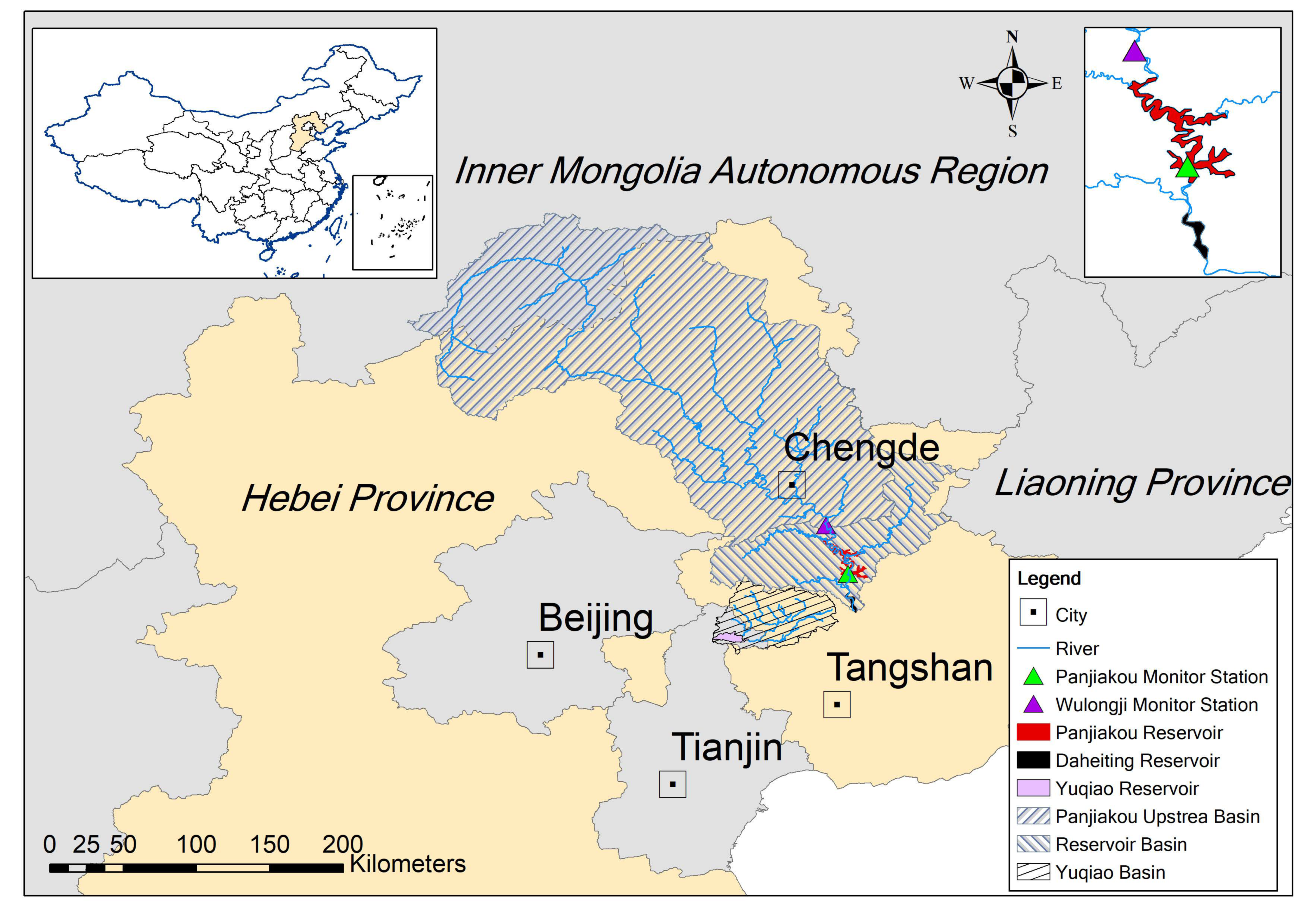
2.1. Study Area
2.2. Data Sources
2.3. Statistical Methods
2.4. LAKE2K Model
3. Results and Discussion
3.1. Long-Term and Seasonal Trend of Water Quality
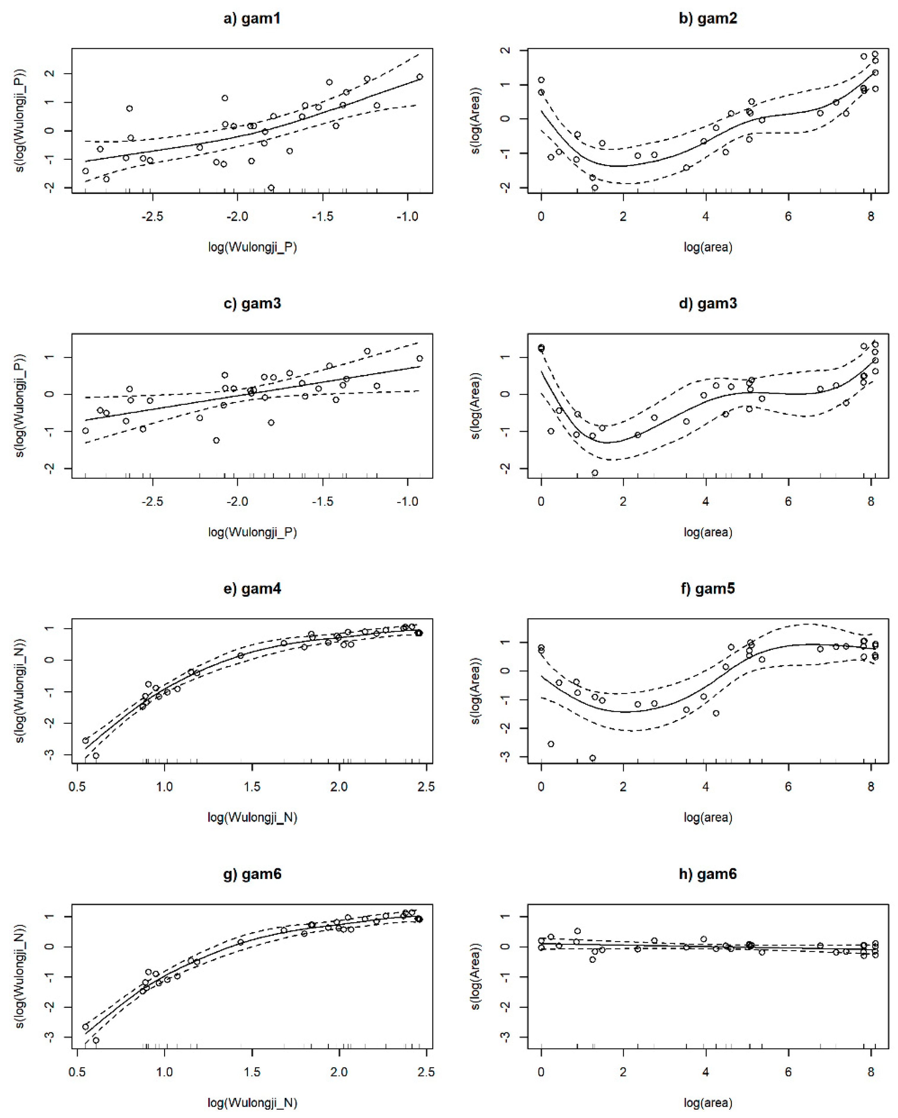
3.2. GAM Results
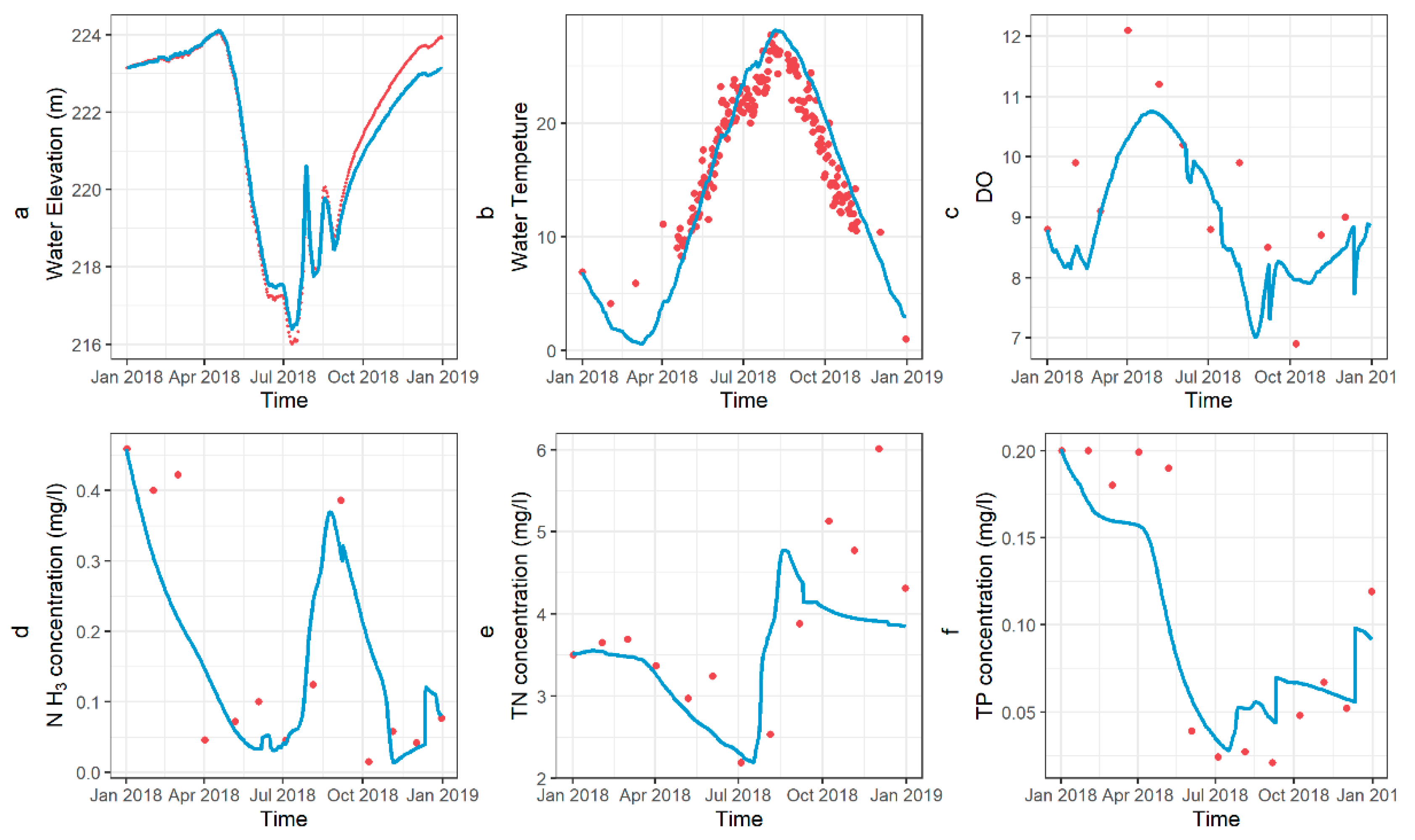
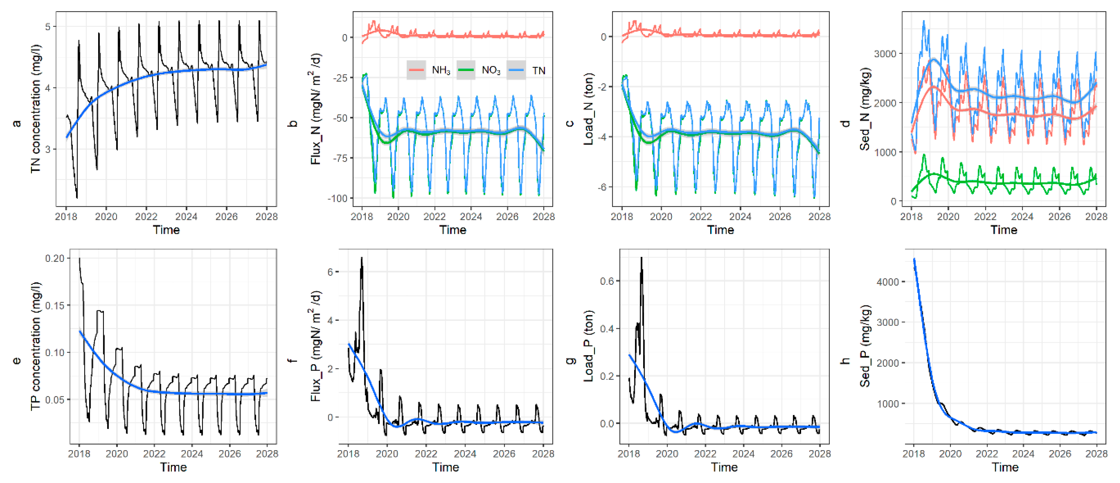
3.3. LAKE2K Model
4. Conclusions
Supplementary Materials
Author Contributions
Funding
Conflicts of Interest
References
- Wang, Y.; Zhang, W.; Zhao, Y.; Peng, H.; Shi, Y. Modelling water quality and quantity with the influence of inter-basin water diversion projects and cascade reservoirs in the Middle-lower Hanjiang River. J. Hydrol. 2016, 541, 1348–1362. [Google Scholar] [CrossRef]
- Zeng, Q.H.; Qin, L.H.; Li, X.Y. The potential impact of an inter-basin water transfer project on nutrients (nitrogen and phosphorous) and chlorophyll a of the receiving water system. Sci. Total Environ. 2015, 536, 675–686. [Google Scholar] [CrossRef]
- Domagalski, J.; Lin, C.; Luo, Y.; Kang, J.; Wang, S.; Brown, L.R.; Munn, M.D. Eutrophication study at the Panjiakou-Daheiting reservoir system, northern Hebei province, people’s republic of China: Chlorophyll-a model and sources of phosphorus and nitrogen. Agric. Water Manag. 2007, 94, 43–53. [Google Scholar] [CrossRef]
- Wang, J.; Zhou, Y.; Xiao, W.; Huang, Y.; Bi, Y.; Wang, L.; Yang, Z. Spatiotemporal Variability of Algae in Monitoring Aquatic Environment in the Panjiakou Reservoir (Northern China). Water Resour. 2016, 43, 690–698. [Google Scholar] [CrossRef] [Green Version]
- Li, Y.; Gao, B.; Xu, D.; Peng, W.; Liu, X.; Qu, X.; Zhang, M. Hydrodynamic impact on trace metals in sediments in the cascade reservoirs, North China. Sci. Total Environ. 2020, 716. [Google Scholar] [CrossRef]
- Wen, S.; Wang, H.; Wu, T.; Yang, J.; Jiang, X.; Zhong, J. Vertical profiles of phosphorus fractions in the sediment in a chain of reservoirs in North China: Implications for pollution source, bioavailability, and eutrophication. Sci. Total Environ. 2020, 704. [Google Scholar] [CrossRef] [PubMed]
- Cao, B.; Dai, Y.; Zhu, L.; Li, C.; Liu, Y.; Wang, Y. Study on simulation of influence of fish cage culture on water quality in riverine reservoir. J. Water Resour. Water Eng. 2016, 27, 75–81. [Google Scholar]
- Liu, X.; Wang, S.; Liu, S.; Lv, Y. Cause Analysis on Algae Outbreak in Panjiakou and Daheiting Reservoirs and Discussion of Protective Countermeasures. Haihe Water Resour. 2019, 05, 1–3+5. [Google Scholar]
- Zhai, W.; Wang, S. Discussion on the protection of water sources in Panjiakou and Daheiting reservoirs. Tech. Superv. Water Resour. 2018, 6, 15–17+51. [Google Scholar]
- Wan, Y.; Wan, L.; Li, Y.; Doering, P. Decadal and seasonal trends of nutrient concentration and export from highly managed coastal catchments. Water Res. 2017, 115, 180–194. [Google Scholar] [CrossRef]
- Hirsch, R.M.; Alexander, R.B.; Smith, R.A. Selection of methods for the detection and estimation of trends in water quality. Water Resour. Res. 1991, 27, 803–813. [Google Scholar] [CrossRef]
- Morton, R.; Henderson, B.L. Estimation of nonlinear trends in water quality: An improved approach using generalized additive models. Water Resour. Res. 2008, 44. [Google Scholar] [CrossRef]
- Cheng, P.; Li, X.Y.; Su, J.J.; Hao, S.N. Recent water quality trends in a typical semi-arid river with a sharp decrease in streamflow and construction of sewage treatment plants. Environ. Res. Lett. 2018, 13, 10. [Google Scholar] [CrossRef] [Green Version]
- Cleveland, R.B.; Cleveland, W.S.; McRae, J.E.; Terpenning, I. STL: A seasonal-trend decomposition. J. Off. Stat. 1990, 6, 3–33. [Google Scholar]
- Huang, H.; Wang, Z.F.; Xia, F.; Shang, X.; Liu, Y.Y.; Zhang, M.H.; Mei, K. Water quality trend and change-point analyses using integration of locally weighted polynomial regression and segmented regression. Environ. Sci. Pollut. Res. 2017, 24, 15827–15837. [Google Scholar] [CrossRef] [PubMed] [Green Version]
- Yang, G.; Moyer, D.L. Estimation of nonlinear water-quality trends in high-frequency monitoring data. Sci. Total Environ. 2020, 715. [Google Scholar] [CrossRef]
- Yee, T.W.; Mitchell, N.D. Generalized additive models in plant ecology. J. Veg. Sci. 1991, 2, 587–602. [Google Scholar] [CrossRef]
- He, S.; Mazumdar, S.; Arena, V.C. A comparative study of the use of GAM and GLM in air pollution research. Environmetrics 2006, 17, 81–93. [Google Scholar] [CrossRef]
- Murphy, R.R.; Perry, E.; Harcum, J.; Keisman, J. A Generalized Additive Model approach to evaluating water quality: Chesapeake Bay case study. Environ. Model. Softw. 2019, 118, 1–13. [Google Scholar] [CrossRef]
- Matisoff, G.; Kaltenberg, E.M.; Steely, R.L.; Hummel, S.K.; Seo, J.; Gibbons, K.J.; Chaffin, J.D. Internal loading of phosphorus in western Lake Erie. J. Great Lakes Res. 2016, 42, 775–788. [Google Scholar] [CrossRef]
- McCulloch, J.; Gudimov, A.; Arhonditsis, G.; Chesnyuk, A.; Dittrich, M. Dynamics of P-binding forms in sediments of a mesotrophic hard-water lake: Insights from non-steady state reactive-transport modeling, sensitivity and identifiability analysis. Chem. Geol. 2013, 354, 216–232. [Google Scholar] [CrossRef]
- Dittrich, M.; Chesnyuk, A.; Gudimo, A.; McCulloch, J.; Quazi, S.; Young, J.; Arhonditsis, G. Phosphorus retention in a mesotrophic lake under transient loading conditions: Insights from a sediment phosphorus binding form study. Water Res. 2013, 47, 1433–1447. [Google Scholar] [CrossRef] [PubMed]
- Doan, P.T.K.; Watson, S.B.; Markovic, S.; Liang, A.Q.; Guo, J.; Mugalingam, S.; Dittrich, M. Phosphorus retention and internal loading in the Bay of Quinte, Lake Ontario, using diagenetic modelling. Sci. Total Environ. 2018, 636, 39–51. [Google Scholar] [CrossRef] [PubMed]
- Qin, L.H.; Zeng, Q.H.; Zhang, W.S.; Li, X.Y.; Steinman, A.D.; Du, X.Z. Estimating internal P loading in a deep water reservoir of northern China using three different methods. Environ. Sci. Pollut. Res. 2016, 23, 18512–18523. [Google Scholar] [CrossRef] [PubMed]
- Luff, R.; Moll, A. Seasonal dynamics of the North Sea sediments using a three-dimensional coupled sediment-water model system. Cont. Shelf Res. 2004, 24, 1099–1127. [Google Scholar] [CrossRef]
- Liu, X.; Wang, Y.; Feng, J.; Chu, C.; Qiu, Y.; Xu, Z.; Wang, Y. A Bayesian modeling approach for phosphorus load apportionment in a reservoir with high water transfer disturbance. Environ. Sci. Pollut. Res. 2018, 25, 32395–32408. [Google Scholar] [CrossRef]
- Lewis, G.N.; Auer, M.T.; Xiang, X.Y.; Penn, M.R. Modeling phosphorus flux in the sediments of Onondaga Lake: Insights on the timing of lake response and recovery. Ecol. Model. 2007, 209, 121–135. [Google Scholar] [CrossRef]
- Epstein, D.M.; Neilson, B.T.; Goodman, K.J.; Stevens, D.K.; Wurtsbaugh, W.A. A modeling approach for assessing the effect of multiple alpine lakes in sequence on nutrient transport. Aquat. Sci. 2013, 75, 199–212. [Google Scholar] [CrossRef]
- Chapra, S.C.; Martin, J.L. LAKE2K: A Modeling Framework for Simulating Lake Water Quality (Version 1.4): Documentation and Users Manual; Civil and Environmental Engineering Department, Tufts University Medford: Medford, MA, USA, 2012. [Google Scholar]
- Cheng, Y.; Feng, P.; Li, J.; Guo, Y.; Ren, P. Water Supply Risk Analysis Based on Runoff Sequence Simulation with Change Point under Changing Environment. Adv. Meteorol. 2019, 2019, 9619254. [Google Scholar] [CrossRef]
- Li, J.; Zhou, S. Quantifying the contribution of climate- and human-induced runoff decrease in the Luanhe river basin, China. J. Water Clim. Chang. 2015, 7, 430–442. [Google Scholar] [CrossRef]
- Cleveland, W.S.; Devlin, S.J. Locally Weighted Regression: An Approach to Regression Analysis by Local Fitting. J. Am. Stat. Assoc. 1988, 83, 596–610. [Google Scholar] [CrossRef]
- Xu, J.; Jin, G.Q.; Tang, H.W.; Zhang, P.; Wang, S.; Wang, Y.G.; Li, L. Assessing temporal variations of Ammonia Nitrogen concentrations and loads in the Huaihe River Basin in relation to policies on pollution source control. Sci. Total Environ. 2018, 642, 1386–1395. [Google Scholar] [CrossRef] [PubMed]
- Tukey, J.W. Exploratory Data Analysis; Addison-Wesley: Reading, MA, USA, 1977. [Google Scholar]
- Hastie, T.J.; Tibshirani, R.J. Generalized Additive Models; Chapman and Hall/CRC: Boca Raton, FL, USA, 1990. [Google Scholar]
- Underwood, F.M. Describing long-term trends in precipitation using generalized additive models. J. Hydrol. 2009, 364, 285–297. [Google Scholar] [CrossRef]
- Ross, N. A Free, Interactive Course Using Mgcv. 2020. Available online: https://noamross.github.io/gams-in-r-course/ (accessed on 10 September 2020).
- McCrthy, S. Modeling the Physical and Biogeochemical Processes in Lake Superior Using LAKE2K. Master’s Thesis, Michigan Technological University, Houghton, MI, USA, 2016. [Google Scholar]
- Allam, A.; Tawfik, A.; Yoshimura, C.; Fleifle, A. Simulation-based optimization framework for reuse of agricultural drainage water in irrigation. J. Environ. Manag. 2016, 172, 82–96. [Google Scholar] [CrossRef]
- Qian, S.S.; Borsuk, M.E.; Stow, C.A. Seasonal and long-term nutrient trend decomposition along a spatial gradient in the Neuse River watershed. Environ. Sci. Technol. 2000, 34, 4474–4482. [Google Scholar] [CrossRef]
- Huang, J.J.; Xiang, W. Investigation of point source and non-point source pollution for Panjiakou Reservoir in North China by modelling approach. Water Qual. Res. J. Can. 2015, 50, 167–181. [Google Scholar] [CrossRef]
- Xie, H.; Chen, L.; Shen, Z. Assessment of Agricultural Best Management Practices Using Models: Current Issues and Future Perspectives. Water 2015, 7, 1088–1108. [Google Scholar] [CrossRef] [Green Version]
- Qi, Z.; Kang, G.; Wu, X.; Sun, Y.; Wang, Y. Multi-Objective Optimization for Selecting and Siting the Cost-Effective BMPs by Coupling Revised GWLF Model and NSGAII Algorithm. Water 2020, 12, 235. [Google Scholar] [CrossRef] [Green Version]
- Kang, G.; Qiu, Y.; Wang, Q.; Qi, Z.; Sun, Y.; Wang, Y. Exploration of the critical factors influencing the water quality in two contrasting climatic regions. Environ. Sci. Pollut. Res. 2020, 27, 12601–12612. [Google Scholar] [CrossRef]
- Parmar, D.L.; Keshari, A.K. Sensitivity analysis of water quality for Delhi stretch of the River Yamuna, India. Environ. Monit. Assess. 2012, 184, 1487–1508. [Google Scholar] [CrossRef]
- Zhu, X.; Zhang, M.; Qu, X.-d.; Peng, W.-q.; Duan, L.-f. Contamination status and speciation for the sediment nutrients in Panjiakou- Daheiting Reservoir. Chin. J. Appl. Ecol. 2018, 29, 3847–3856. [Google Scholar] [CrossRef]
- Williams, V.P. Effects of Point-Source Removal on Lake Water Quality: A Case History of Lake Tohopekaliga, Florida. Lake Reserv. Manag. 2001, 17, 315–329. [Google Scholar] [CrossRef]
- Zhang, H.; Boegman, L.; Scavia, D.; Culver, D.A. Spatial distributions of external and internal phosphorus loads in Lake Erie and their impacts on phytoplankton and water quality. J. Great Lakes Res. 2016, 42, 1212–1227. [Google Scholar] [CrossRef]
- Turner, R.E.; Rabalais, N.N.; Justic, D. Gulf of Mexico Hypoxia: Alternate States and a Legacy. Environ. Sci. Technol. 2008, 42, 2323–2327. [Google Scholar] [CrossRef] [PubMed]
- Nurnberg, G.K.; LaZerte, B.D. Modeling the effect of development on internal phosphorus load in nutrient-poor lakes. Water Resour. Res. 2004, 40. [Google Scholar] [CrossRef] [Green Version]
- Phillips, G.; Kelly, A.; Pitt, J.A.; Sanderson, R.; Taylor, E. The recovery of a very shallow eutrophic lake, 20 years after the control of effluent derived phosphorus. Freshw. Biol. 2005, 50, 1628–1638. [Google Scholar] [CrossRef]
- Jeppesen, E.; Sondergaard, M.; Jensen, J.P.; Havens, K.E.; Anneville, O.; Carvalho, L.; Winder, M. Lake responses to reduced nutrient loading—An analysis of contemporary long-term data from 35 case studies. Freshw. Biol. 2005, 50, 1747–1771. [Google Scholar] [CrossRef]
- Capon, S.J.; Lynch, A.J.J.; Bond, N.; Chessman, B.C.; Davis, J.; Davidson, N.; Nally, R.M. Regime shifts, thresholds and multiple stable states in freshwater ecosystems; a critical appraisal of the evidence. Sci. Total Environ. 2015, 534, 122–130. [Google Scholar] [CrossRef] [Green Version]
- Li, N.; Zhang, X.; Wu, W.; Zhao, X. Occurrence, seasonal variation and risk assessment of antibiotics in the reservoirs in North China. Chemosphere 2014, 111, 327–335. [Google Scholar] [CrossRef]


| Models | R2-Adj | Deviance Explained | AIC 1 | Linear Term 1 | s(log(Wulongji_P) 2 | s(log(Wulongji_N) 2 | s(Area) 2 |
|---|---|---|---|---|---|---|---|
| gam1 | 0.48 | 51.1% | 78.840 | −3.4121 *** | 1.85 *** | NA | NA |
| gam2 | 0.758 | 79.5% | 57.783 | −3.41209 *** | NA | NA | 4.744 *** |
| gam3 | 0.805 | 84.4% | 51.520 | −3.41209 *** | 1.000 * | NA | 5.261 *** |
| gam4 | 0.968 | 97.2% | −5.168 | 0.65616 *** | NA | 4.259 *** | NA |
| gam5 | 0.589 | 64.2% | 76.719 | 0.6562 *** | NA | NA | 3.958 *** |
| gam6 | 0.969 | 97.4% | −5.184 | 0.65616 *** | NA | 4.3 *** | 1.000 |
| Variables | Water Elevation | Water Temperature | DO | Nitrogen | TN | TP |
|---|---|---|---|---|---|---|
| Unit | m | °C | mg/L | mg/L | mg/L | mg/L |
| Observed mean | 68.35 | 13.53 | 8.90 | 13.53 | 3.47 | 0.09 |
| Modeled mean | 68.51 | 14.77 | 9.43 | 14.77 | 3.79 | 0.11 |
| RMSE | 0.42 | 3.12 | 0.91 | 0.09 | 0.83 | 0.03 |
Publisher’s Note: MDPI stays neutral with regard to jurisdictional claims in published maps and institutional affiliations. |
© 2020 by the authors. Licensee MDPI, Basel, Switzerland. This article is an open access article distributed under the terms and conditions of the Creative Commons Attribution (CC BY) license (http://creativecommons.org/licenses/by/4.0/).
Share and Cite
Kang, G.; Yin, J.; Cui, N.; Ding, H.; Wang, S.; Wang, Y.; Qi, Z. The Long-Term and Retention Impacts of the Intervention Policy for Cage Aquaculture on the Reservoir Water Qualities in Northern China. Water 2020, 12, 3325. https://doi.org/10.3390/w12123325
Kang G, Yin J, Cui N, Ding H, Wang S, Wang Y, Qi Z. The Long-Term and Retention Impacts of the Intervention Policy for Cage Aquaculture on the Reservoir Water Qualities in Northern China. Water. 2020; 12(12):3325. https://doi.org/10.3390/w12123325
Chicago/Turabian StyleKang, Gelin, Jingchen Yin, Naixin Cui, Han Ding, Shaoming Wang, Yuqiu Wang, and Zuoda Qi. 2020. "The Long-Term and Retention Impacts of the Intervention Policy for Cage Aquaculture on the Reservoir Water Qualities in Northern China" Water 12, no. 12: 3325. https://doi.org/10.3390/w12123325
APA StyleKang, G., Yin, J., Cui, N., Ding, H., Wang, S., Wang, Y., & Qi, Z. (2020). The Long-Term and Retention Impacts of the Intervention Policy for Cage Aquaculture on the Reservoir Water Qualities in Northern China. Water, 12(12), 3325. https://doi.org/10.3390/w12123325