Development and Evaluation of the Combined Machine Learning Models for the Prediction of Dam Inflow

 ,
,  ,
,  and
and 
Abstract
1. Introduction
2. Methodology
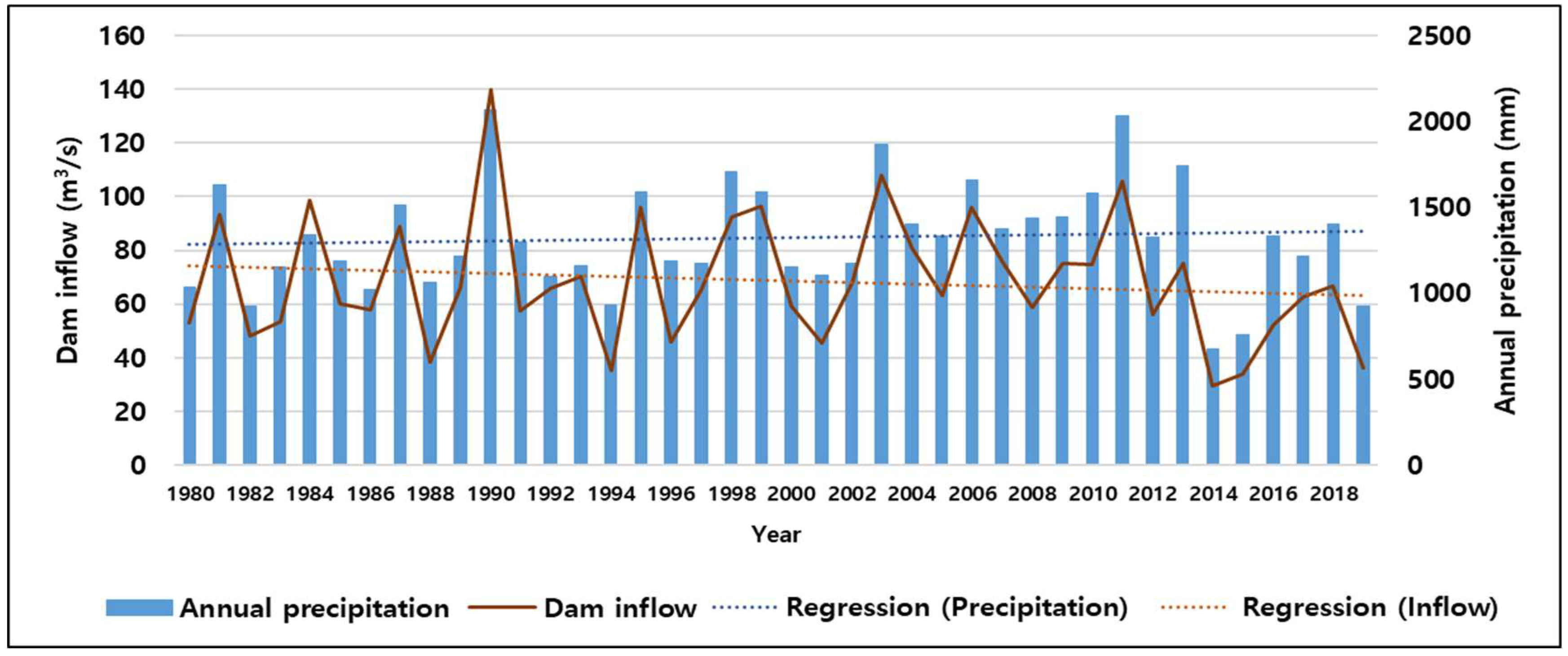
2.1. Study Area
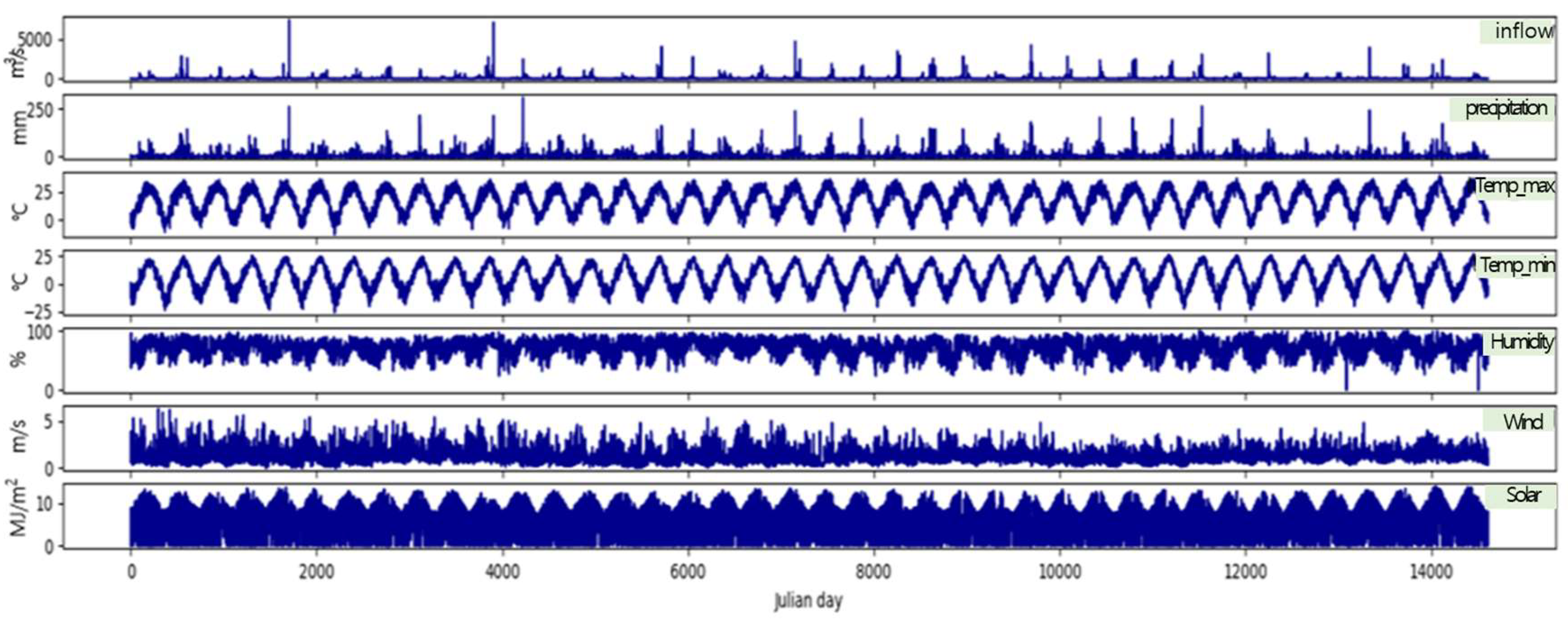
2.2. Data Descriptions
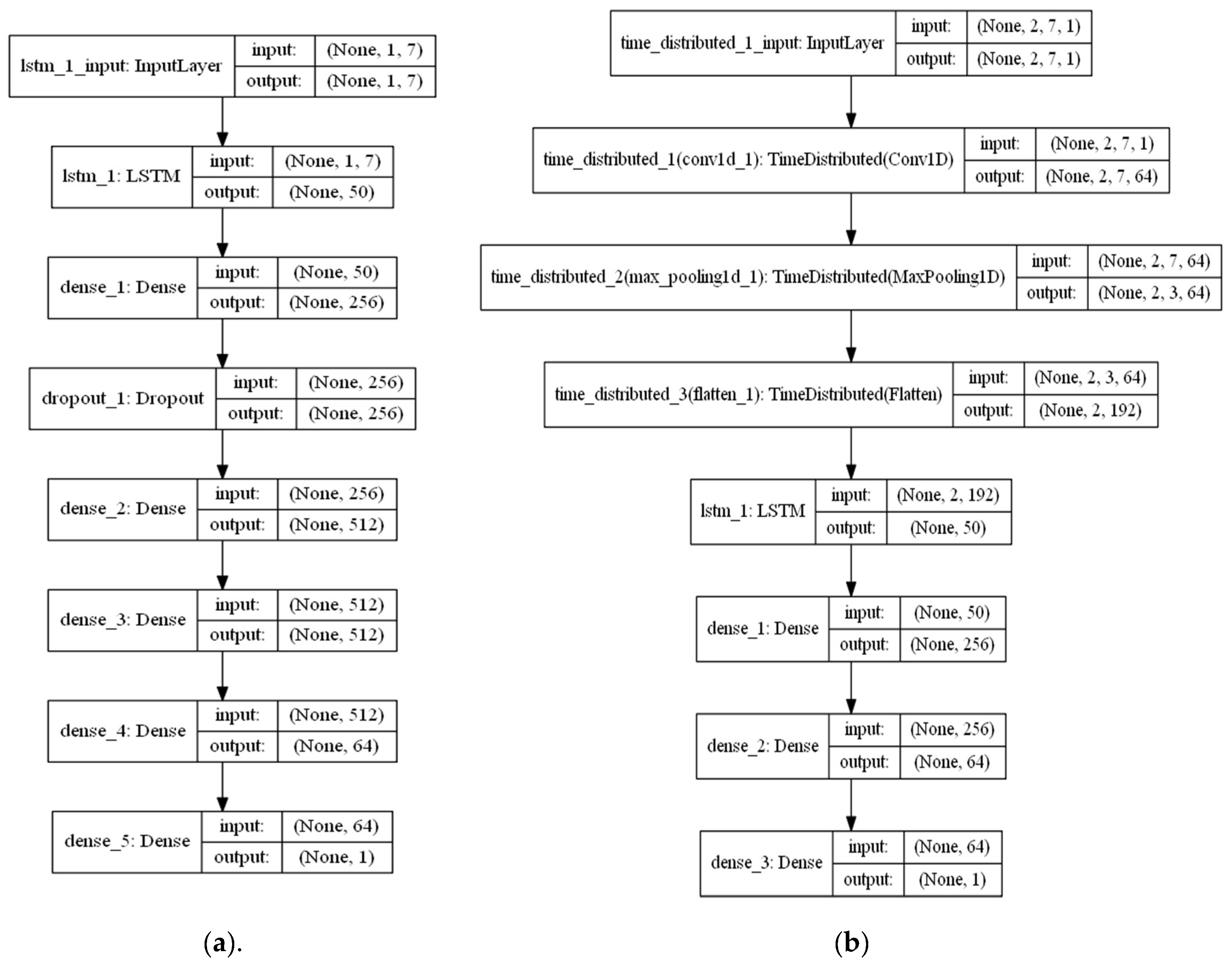
2.3. Machine Learning Algorithms
2.4. Development of Combined Machine Learning Algorithms (CombML)
2.5. Model Training Test
3. Results and Discussion
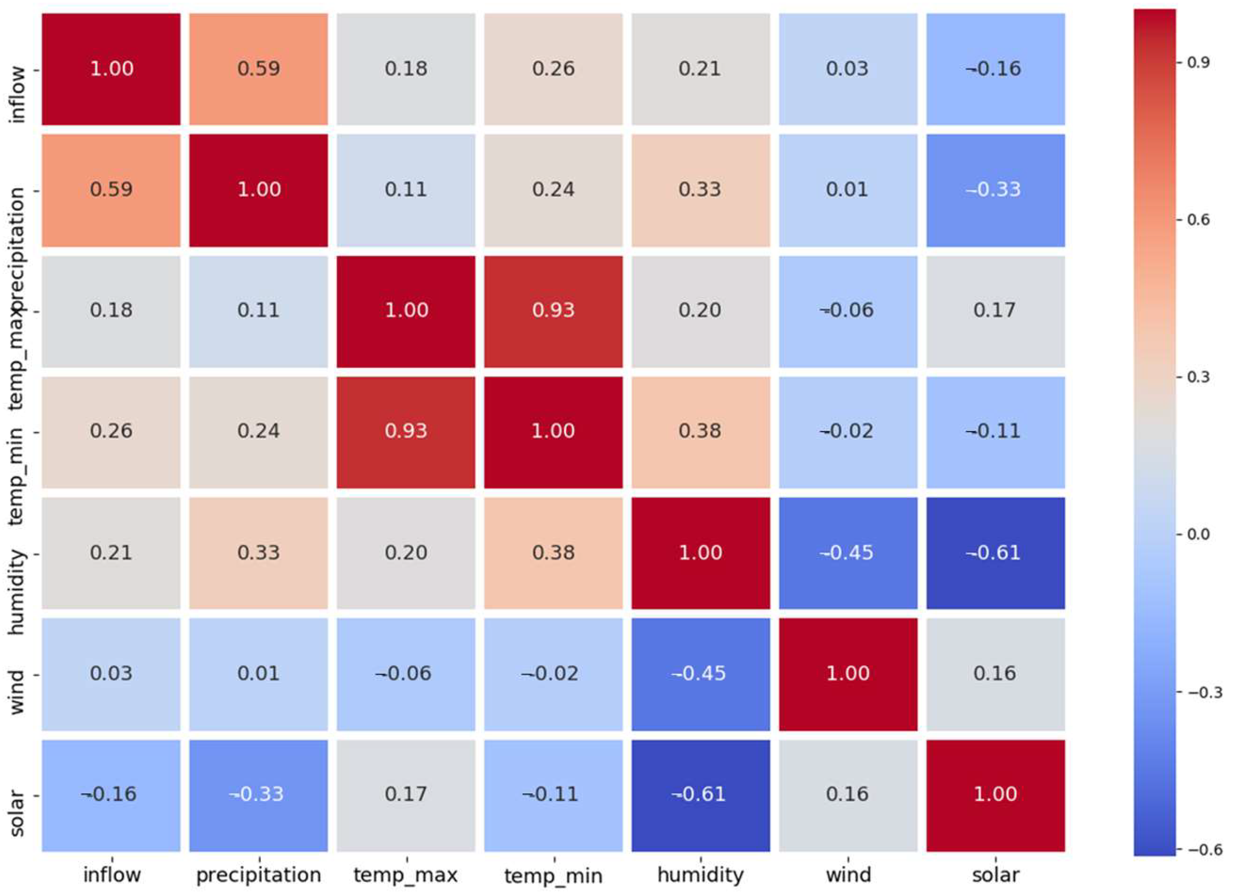
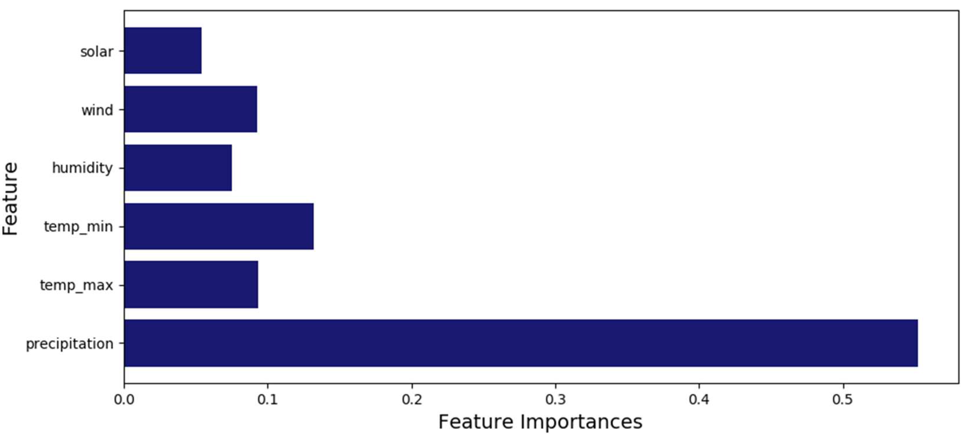
3.1. Impact Factor Analysis
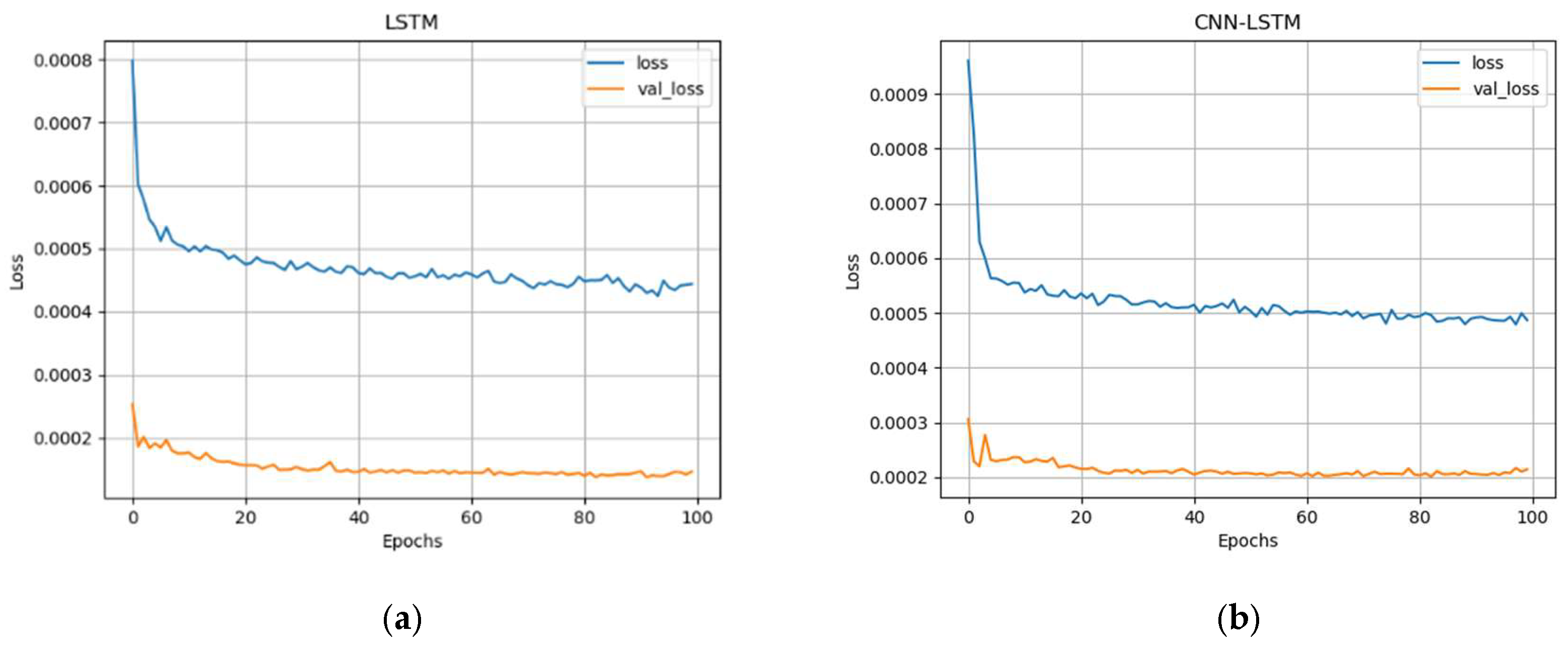
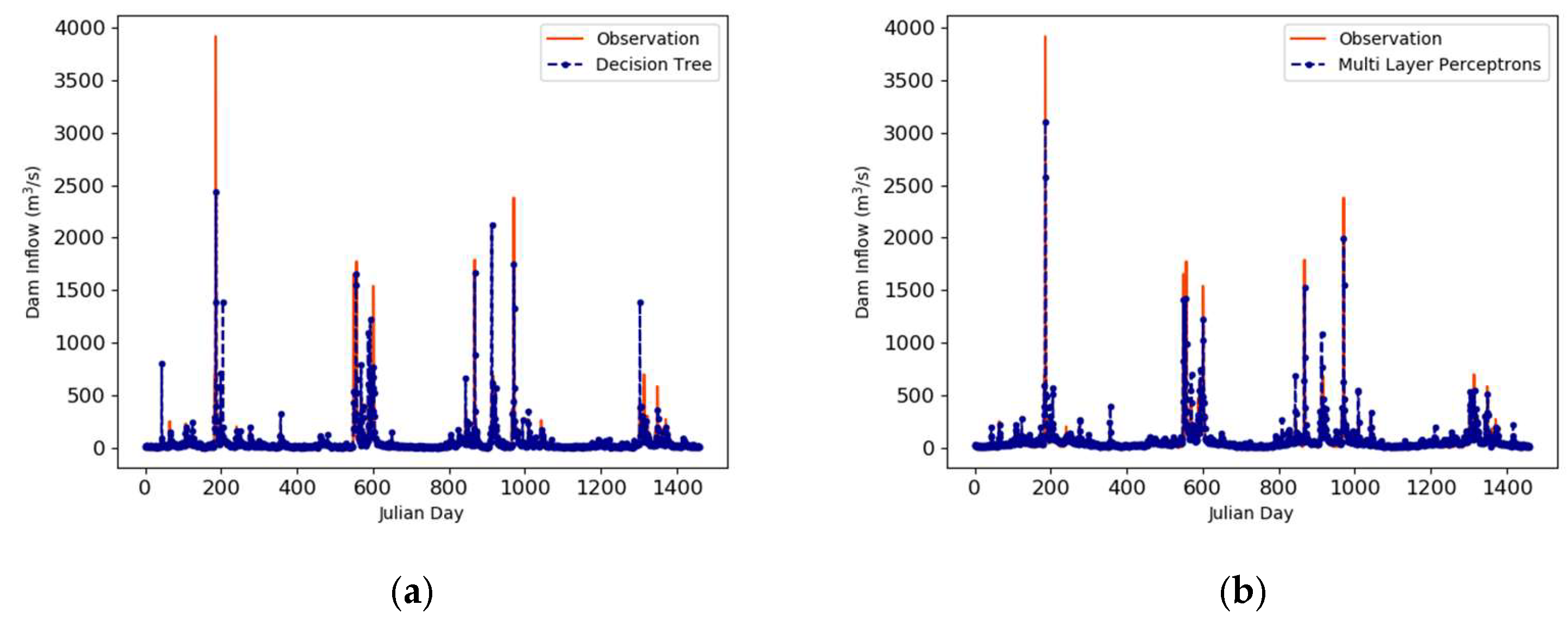
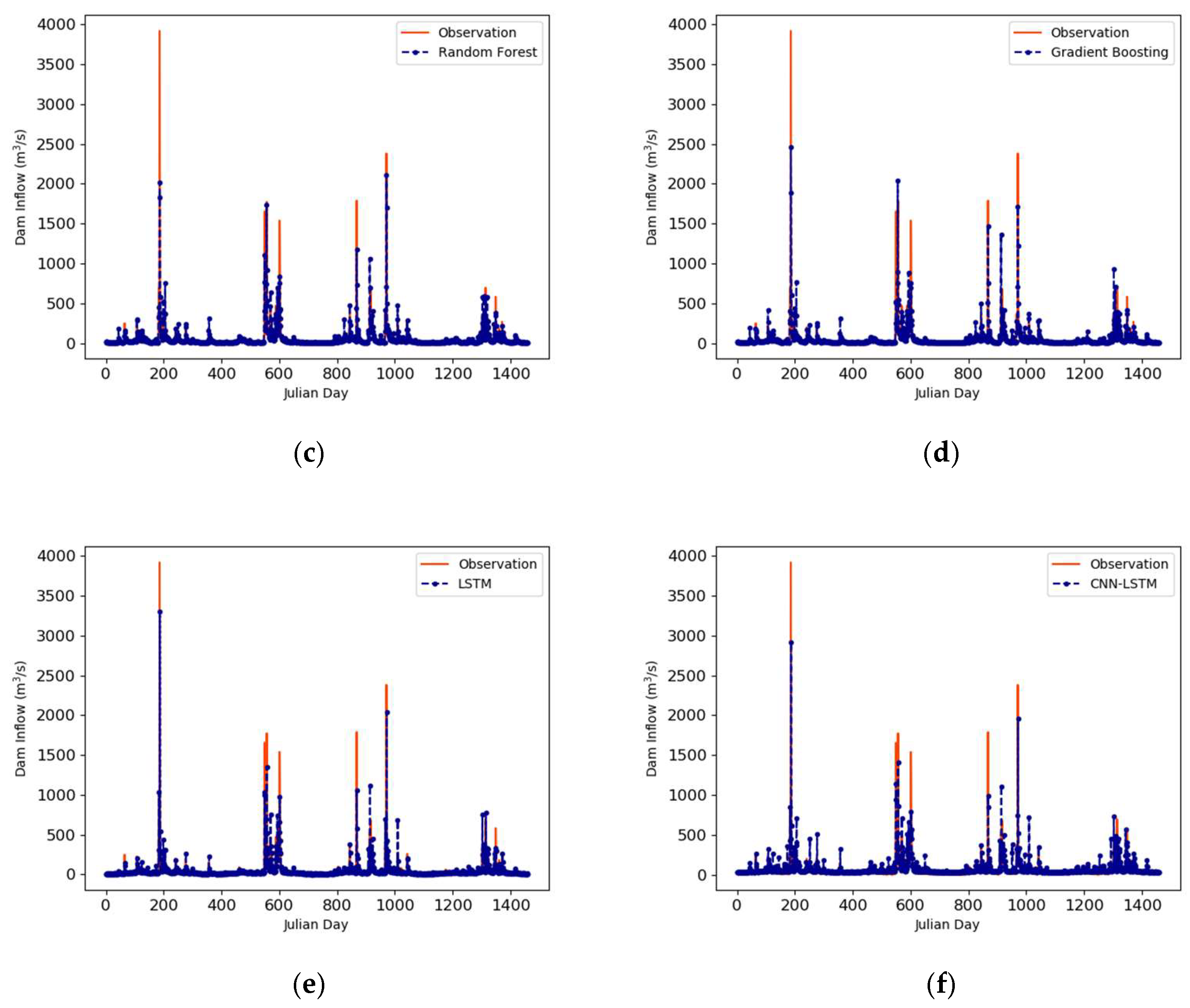
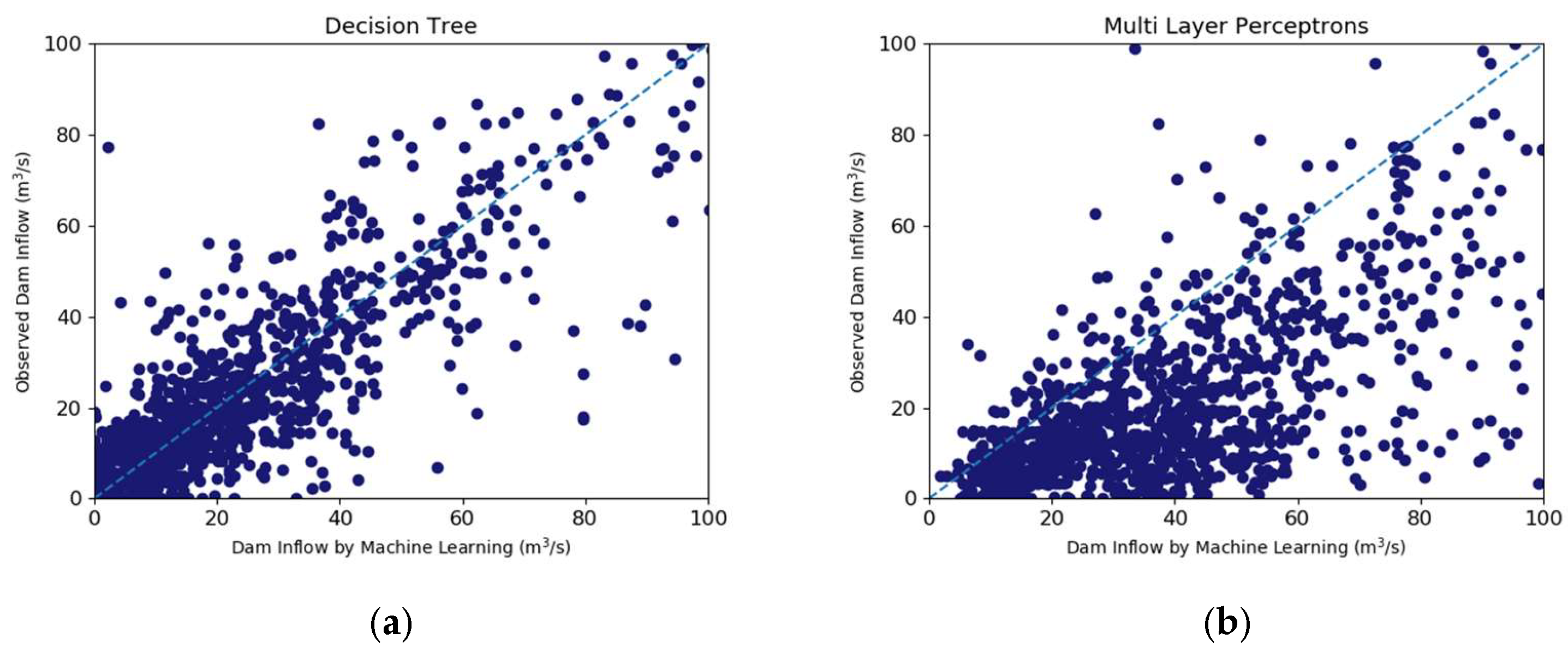
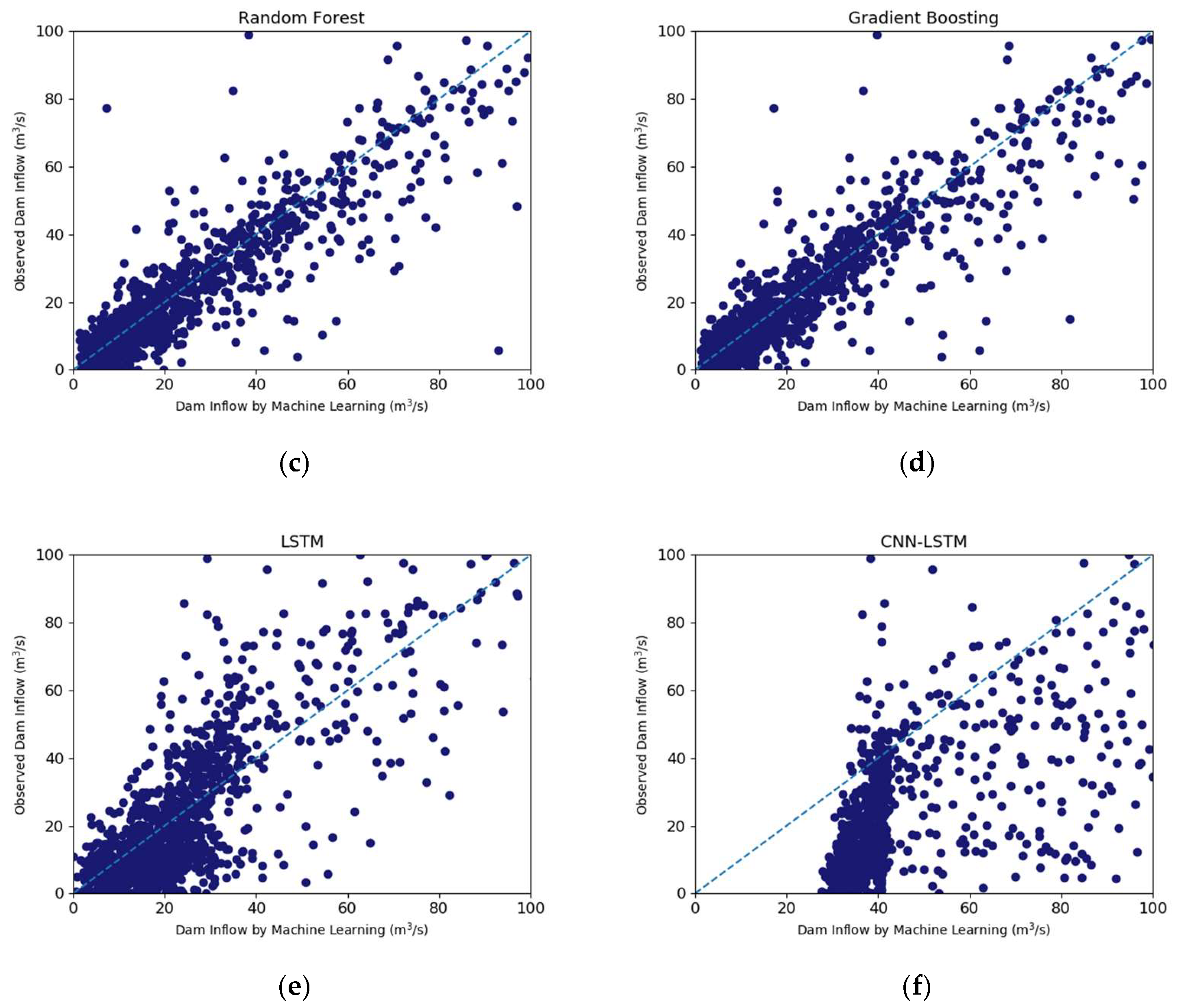
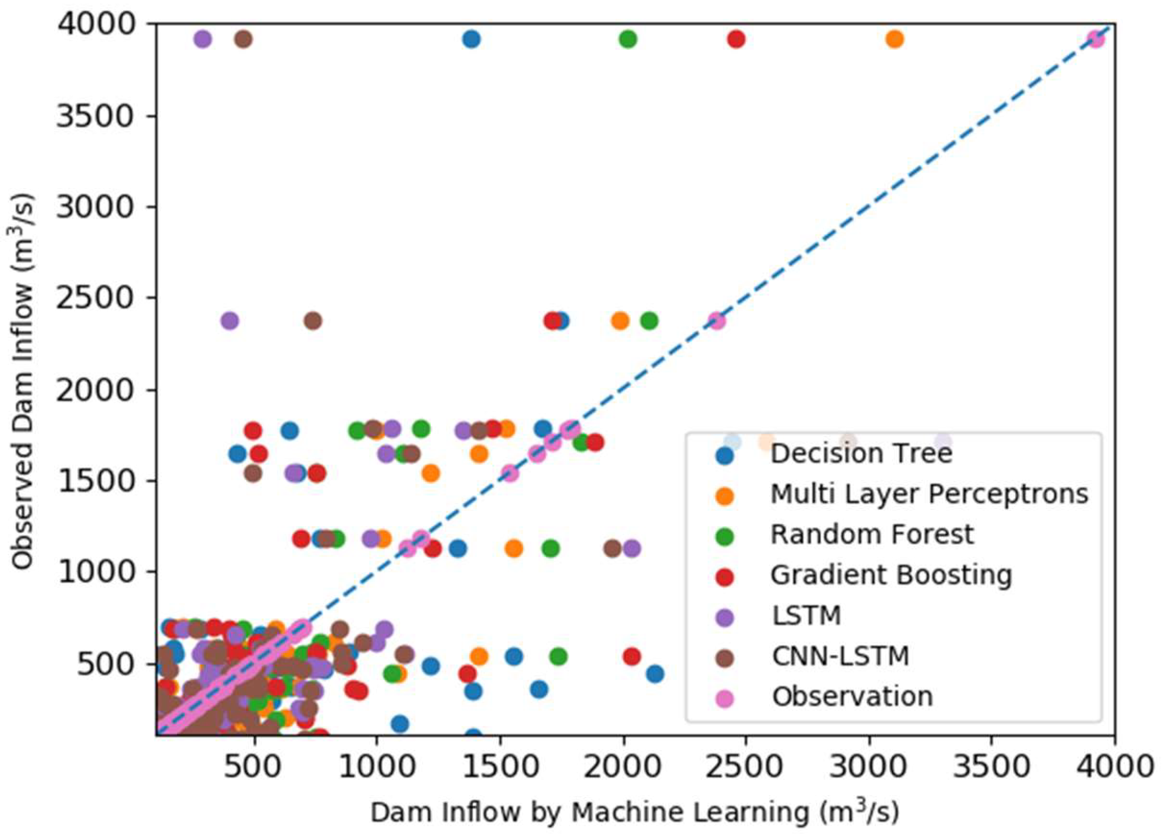
3.2. Prediction Results Using Machine Learning Algorithms
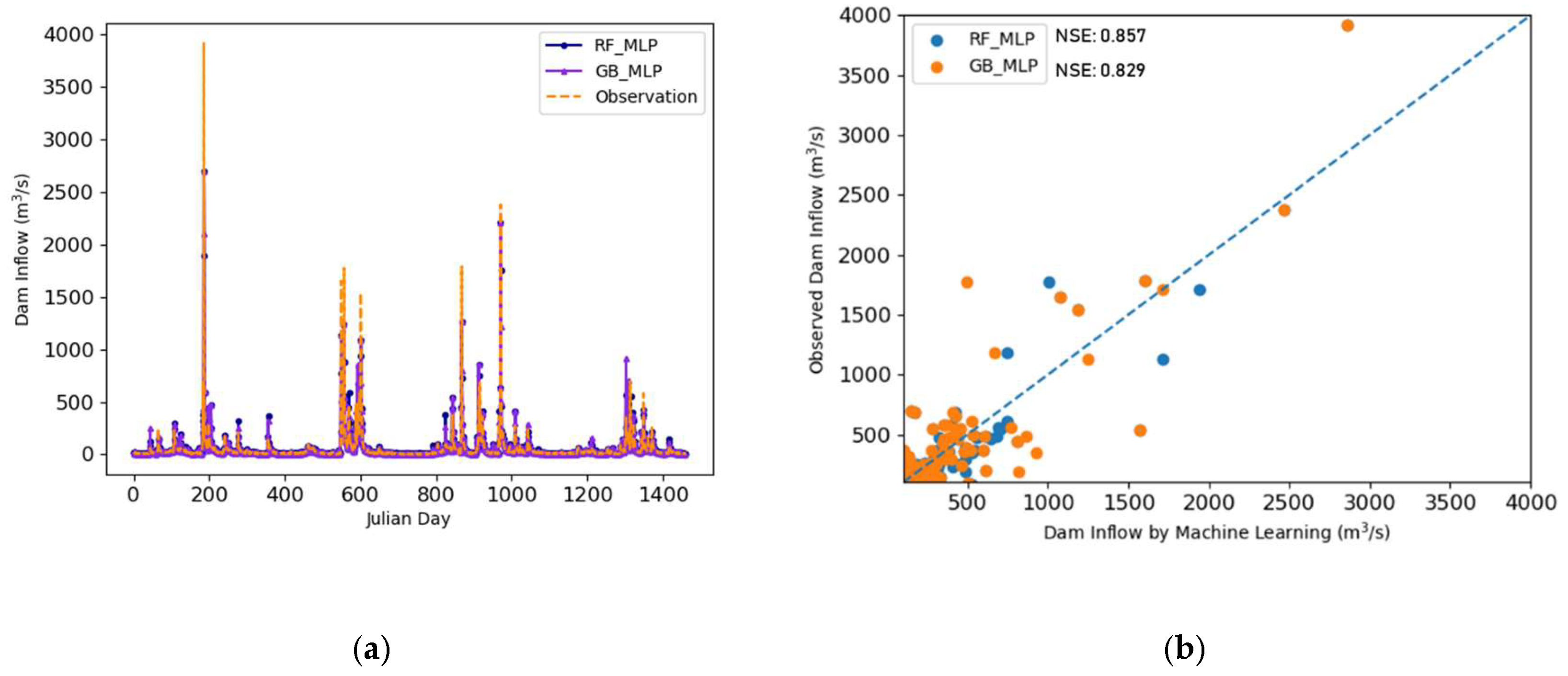
3.3. Prediction Results Using CombML
4. Conclusions
Author Contributions
Funding
Conflicts of Interest
References
- Donnelly, C.; Greuell, W.; Andersson, J.; Gerten, D.; Pisacane, G.; Roudier, P.; Ludwig, F. Impacts of climate change on European hydrology at 1.5, 2 and 3 degrees mean global warming above preindustrial level. Clim. Chang. 2017, 143, 13–26. [Google Scholar] [CrossRef]
- Choi, I.-C.; Shin, H.-J.; Nguyen, T.T.; Tenhunen, J. Water policy reforms in South Korea: A historical review and ongoing challenges for sustainable water governance and management. Water 2017, 9, 717. [Google Scholar] [CrossRef]
- Ahn, J.M.; Jung, K.Y.; Shin, D. Effects of coordinated operation of weirs and reservoirs on the water quality of the Geum River. Water 2017, 9, 423. [Google Scholar]
- Park, J.Y.; Kim, S.J. Potential impacts of climate change on the reliability of water and hydropower supply from a multipurpose dam in South Korea. JAWRA J. Am. Water Resour. Assoc. 2014, 50, 1273–1288. [Google Scholar] [CrossRef]
- Lee, J.E.; Heo, J.-H.; Lee, J.; Kim, N.W. Assessment of flood frequency alteration by dam construction via SWAT Simulation. Water 2017, 9, 264. [Google Scholar] [CrossRef]
- Ryu, J.; Jang, W.S.; Kim, J.; Choi, J.D.; Engel, B.A.; Yang, J.E.; Lim, K.J. Development of a watershed-scale long-term hydrologic impact assessment model with the asymptotic curve number regression equation. Water 2016, 8, 153. [Google Scholar] [CrossRef]
- Stern, M.; Flint, L.; Minear, J.; Flint, A.; Wright, S. Characterizing changes in streamflow and sediment supply in the Sacramento River Basin, California, using hydrological simulation program—FORTRAN (HSPF). Water 2016, 8, 432. [Google Scholar] [CrossRef]
- Nyeko, M. Hydrologic modelling of data scarce basin with SWAT Model: Capabilities and limitations. Water Resour. Manag. 2015, 29, 81–94. [Google Scholar] [CrossRef]
- Zhao, F.; Wu, Y.; Qiu, L.; Sun, Y.; Sun, L.; Li, Q.; Niu, J.; Wang, G. Parameter uncertainty analysis of the SWAT model in a mountain-loess transitional watershed on the Chinese Loess Plateau. Water 2018, 10, 690. [Google Scholar] [CrossRef]
- Lee, G.; Lee, H.W.; Lee, Y.S.; Choi, J.H.; Yang, J.E.; Lim, K.J.; Kim, J. The effect of reduced flow on downstream water systems due to the kumgangsan dam under dry conditions. Water 2019, 11, 739. [Google Scholar] [CrossRef]
- Valipour, M.; Banihabib, M.E.; Behbahani, S.M.R. Comparison of the ARMA, ARIMA, and the autoregressive artificial neural network models in forecasting the monthly inflow of Dez dam reservoir. J. Hydrol. 2013, 476, 433–441. [Google Scholar] [CrossRef]
- Liu, Y.; Wu, J.; Liu, Y.; Hu, B.X.; Hao, Y.; Huo, X.; Fan, Y.; Yeh, T.J.; Wang, Z.-L. Analyzing effects of climate change on streamflow in a glacier mountain catchment using an ARMA model. Quat. Int. 2015, 358, 137–145. [Google Scholar] [CrossRef]
- Myronidis, D.; Ioannou, K.; Fotakis, D.; Dörflinger, G. Streamflow and hydrological drought trend analysis and forecasting in Cyprus. Water Resour. Manag. 2018, 32, 1759–1776. [Google Scholar] [CrossRef]
- Rezaie-Balf, M.; Naganna, S.R.; Kisi, O.; El-Shafie, A. Enhancing streamflow forecasting using the augmenting ensemble procedure coupled machine learning models: Case study of Aswan High Dam. Hydrol. Sci. J. 2019, 64, 1629–1646. [Google Scholar] [CrossRef]
- Balaguer, E.; Palomares, A.; Soria, E.; Martín-Guerrero, J.D. Predicting service request in support centers based on nonlinear dynamics, ARMA modeling and neural networks. Expert Syst. Appl. 2008, 34, 665–672. [Google Scholar] [CrossRef]
- Ali, M.; Qamar, A.M.; Ali, B. Data Analysis, Discharge Classifications, and Predictions of Hydrological Parameters for the Management of Rawal Dam in Pakistan. In Proceedings of the 12th International Conference on Machine Learning and Applications, Miami, FL, USA, 4–7 December 2013; pp. 382–385. [Google Scholar]
- Le, X.-H.; Ho, H.V.; Lee, G.; Jung, S. Application of long short-term memory (LSTM) neural network for flood forecasting. Water 2019, 11, 1387. [Google Scholar] [CrossRef]
- LeCun, Y.; Bengio, Y.; Hinton, G. Deep learning. Nature 2015, 521, 436–444. [Google Scholar] [CrossRef] [PubMed]
- Huang, C.-J.; Kuo, P.-H. A deep cnn-lstm model for particulate matter (PM2.5) forecasting in smart cities. Sensors 2018, 18, 2220. [Google Scholar] [CrossRef] [PubMed]
- Bougoudis, I.; Demertzis, K.; Iliadis, L. HISYCOL a hybrid computational intelligence system for combined machine learning: The case of air pollution modeling in Athens. Neural Comput. Appl. 2016, 27, 1191–1206. [Google Scholar] [CrossRef]
- Tongal, H.; Booij, M.J. Simulation and forecasting of streamflows using machine learning models coupled with base flow separation. J. Hydrol. 2018, 564, 266–282. [Google Scholar] [CrossRef]
- Shortridge, J.E.; Guikema, S.D.; Zaitchik, B.F. Machine learning methods for empirical streamflow simulation: A comparison of model accuracy, interpretability, and uncertainty in seasonal watersheds. Hydrol. Earth Syst. Sci. 2016, 20, 2611–2628. [Google Scholar] [CrossRef]
- Cheng, M.; Fang, F.; Kinouchi, T.; Navon, I.; Pain, C. Long lead-time daily and monthly streamflow forecasting using machine learning methods. J. Hydrol. 2020, 590, 125376. [Google Scholar] [CrossRef]
- Chung, S.-W.; Lee, J.-H.; Lee, H.-S.; Maeng, S.-J. Uncertainty of discharge-SS relationship used for turbid flow modeling. J. Korea Water Resour. Assoc. 2011, 44, 991–1000. [Google Scholar] [CrossRef]
- Jung, I.; Shin, Y.; Park, J.; Kim, D. Increasing Drought Risk in Large-Dam Basins of South Korea. In Proceedings of the AGU Fall Meeting Abstracts, New Orleans, LA, USA, 11–15 December 2017. [Google Scholar]
- Korea Meteorological Administration (KMA). Available online: http://kma.go.kr/home/index.jsp (accessed on 12 February 2020).
- Water Resources Management Information System (WAMIS). Available online: http://www.wamis.go.kr/main.aspx. (accessed on 12 February 2020).
- Woo, W.; Moon, J.; Kim, N.W.; Choi, J.; Kim, K.; Park, Y.S.; Jang, W.S.; Lim, K.J. Evaluation of SATEEC daily R module using daily rainfall. J. Korean Soc. Water Qual. 2010, 26, 841–849. [Google Scholar]
- Bae, J.H.; Han, J.; Lee, D.; Yang, J.E.; Kim, J.; Lim, K.J.; Neff, J.C.; Jang, W.S. Evaluation of sediment trapping efficiency of vegetative filter strips using machine learning models. Sustainability 2019, 11, 7212. [Google Scholar] [CrossRef]
- Kotsiantis, S.; Kanellopoulos, D.; Pintelas, P. Data preprocessing for supervised leaning. Int. J. Comput. Sci. 2006, 1, 111–117. [Google Scholar]
- Teng, C.-M. Correcting Noisy Data. In Proceedings of the 16th Inetrantional Conference on Machine Learning, Bled, Slovenia, 27–30 June 1999; pp. 239–248. [Google Scholar]
- Scikit-Learn. RandomForestRegressor. Available online: https://scikit-learn.org/stable/modules/generated/sklearn.ensemble.RandomForestRegressor.html (accessed on 2 December 2019).
- Thara, D.; PremaSudha, B.; Xiong, F. Auto-detection of epileptic seizure events using deep neural network with different feature scaling techniques. Pattern Recognit. Lett. 2019, 128, 544–550. [Google Scholar]
- Alpaydin, E. Introduction to Machine Learning; MIT Press: Cambridge, MA, USA, 2014. [Google Scholar]
- Breiman, L.; Friedman, J.; Stone, C.J.; Olshen, R.A. Classification and Regression Trees; CRC Press: Boca Raton, FL, USA, 1984. [Google Scholar]
- Azar, A.T.; El-Said, S.A. Probabilistic neural network for breast cancer classification. Neural Comput. Appl. 2013, 23, 1737–1751. [Google Scholar] [CrossRef]
- Moon, J.; Park, S.; Hwang, E. A multilayer perceptron-based electric load forecasting scheme via effective recovering missing data. KIPS Trans. Softw. Data Eng. 2019, 8, 67–78. [Google Scholar]
- Breiman, L. Random forests. Mach. Learn. 2001, 45, 5–32. [Google Scholar] [CrossRef]
- Panchal, G.; Ganatra, A.; Kosta, Y.; Panchal, D. Behaviour analysis of multilayer perceptrons with multiple hidden neurons and hidden layers. Int. J. Comput. Theory Eng. 2011, 3, 332–337. [Google Scholar] [CrossRef]
- Natekin, A.; Knoll, A. Gradient boosting machines, a tutorial. Front. Neurorobot. 2013, 7, 21. [Google Scholar] [CrossRef] [PubMed]
- Hochreiter, S.; Schmidhuber, J. Long short-term memory. Neural Comput. 1997, 9, 1735–1780. [Google Scholar] [CrossRef] [PubMed]
- Chen, Z.; Liu, Y.; Liu, S. Mechanical State Prediction Based on LSTM Neural Netwok. In Proceedings of the 36th Chinese Control Conference (CCC), Dalian, China, 26–28 July 2017; pp. 3876–3881. [Google Scholar]
- Tran, Q.-K.; Song, S.-K. Water level forecasting based on deep learning: A use case of Trinity River-Texas-The United States. J. KIISE 2017, 44, 607–612. [Google Scholar] [CrossRef]
- Fukuoka, R.; Suzuki, H.; Kitajima, T.; Kuwahara, A.; Yasuno, T. Wind Speed Prediction Model Using LSTM and 1D-CNN. J. Signal Process. 2018, 22, 207–210. [Google Scholar] [CrossRef]
- Jung, H.C.; Sun, Y.G.; Lee, D.; Kim, S.H.; Hwang, Y.M.; Sim, I.; Oh, S.K.; Song, S.-H.; Kim, J.Y. Prediction for energy demand using 1D-CNN and bidirectional LSTM in Internet of energy. J. IKEEE 2019, 23, 134–142. [Google Scholar]
- Legates, D.R.; McCabe, G.J., Jr. Evaluating the use of “goodness-of-fit” measures in hydrologic and hydroclimatic model validation. Water Resour. Res. 1999, 35, 233–241. [Google Scholar] [CrossRef]
- Cancelliere, A.; Di Mauro, G.; Bonaccorso, B.; Rossi, G. Drought forecasting using the standardized precipitation index. Water Resour. Manag. 2007, 21, 801–819. [Google Scholar] [CrossRef]
- Moghimi, M.M.; Zarei, A.R. Evaluating performance and applicability of several drought indices in arid regions. Asia-Pacific J. Atmos. Sci. 2019, 1–17. [Google Scholar] [CrossRef]
- Karpagavalli, S.; Jamuna, K.; Vijaya, M. Machine learning approach for preoperative anaesthetic risk prediction. Int. J. Recent Trends Eng. 2009, 1, 19. [Google Scholar]
- Oliveira, T.P.; Barbar, J.S.; Soares, A.S. Computer network traffic prediction: A comparison between traditional and deep learning neural networks. Int. J. Big Data Intell. 2016, 3, 28–37. [Google Scholar] [CrossRef]


| Input Variable | Output Variable | |
|---|---|---|
| Weather Data of Two Days Ago | Inflow (t − 2), precipitation (t − 2), temp_max (t − 2), temp_min (t − 2), humidity (t − 2), wind (t − 2), solar (t − 2) | Inflow of the day: Inflow (t) |
| Weather Data of One Day Ago | Inflow (t − 1), precipitation (t − 1), temp_max (t − 1), temp_min (t − 1), humidity (t − 1), wind (t − 1), solar (t − 1) | |
| Weather Data of the Day (Forecasted) | precipitation (t), temp_max (t), temp_min (t), humidity (t), wind (t), solar (t) |
| Machine Learning Models | Module | Function | Notation |
|---|---|---|---|
| Decision Tree | sklearn.tree | DecisionTreeRegressor | DT |
| Multilayer Perceptron | sklearn.neural_network | MLPRegressor | MLP |
| Random Forest | sklearn.ensemble | RandomForestRegressor | RF |
| Gradient Boosting | sklearn.ensemble | GradientBoostingRegressor | GB |
| RNN–LSTM | keras.models.Sequential | LSTM, Dense, Dropout | LSTM |
| CNN–LSTM | keras.models.Sequential | LSTM, Dense, Dropout, Conv1D, MaxPooling1D | CNN–LSTM |
| Decision Tree Regressor | MLP Regressor | ||
|---|---|---|---|
| Hyperparameter | Value | Hyperparameter | Value |
| Criterion Min_Samples_Leaf Min_Impurity_Decrease Splitter Min_Samples_Split Random_State | Entropy 1 0 Best 2 0 | hidden_layer_sizes solver learning_rate_init max_iter momentum beta_1 epsilon activation | (50,50,50) Adam 0.001 200 0.9 0.9 1 × 10⁻⁸ relu |
| Random Forest Regressor | Gradient Boosting Regressor | ||
| Hyperparameter | Value | Hyperparameter | Value |
| n_Estimators Min_samples_split Min_Weight_Fraction_Leaf Min_Impurity_Decrease Verbose Criterion Min_Samples_Leaf Max_Features Bootstrap | 50 2 0 0 0 Mse 1 Auto True | Loss n_estimators criterion min_samples_leaf max_depth alpha presort tol learning_rate subsample min_samples_split validation_fraction | ls 100 friedman_mse 1 10 0.9 Auto 1 × 10⁻⁴ 0.1 1.0 2 0.1 |
| Method | NSE | RMSE (m3/s) | MAE (m3/s) | R | R2 |
|---|---|---|---|---|---|
| Decision Tree | 0.589 | 114.04 | 27.333 | 0.775 | 0.601 |
| MLP | 0.812 | 77.218 | 29.034 | 0.904 | 0.817 |
| Random Forest | 0.745 | 89.73 | 20.372 | 0.867 | 0.753 |
| Gradient Boosting | 0.718 | 94.486 | 20.522 | 0.848 | 0.718 |
| LSTM | 0.429 | 134.329 | 26.332 | 0.675 | 0.455 |
| CNN–LSTM | 0.455 | 131.243 | 35.921 | 0.694 | 0.482 |
| Date | Observation | DT | MLP | RF | GB | LSTM | CNN-LSTM |
|---|---|---|---|---|---|---|---|
| 5 July 2016 | 3918.50 | 1383.00 | 3106.83 | 2018.88 | 2457.94 | 291.74 | 456.17 |
| 6 July 2016 | 1716.20 | 2443.00 | 2581.32 | 1828.49 | 1886.02 | 3302.50 | 2911.93 |
| 3 July 2017 | 1652.90 | 432.40 | 1410.34 | 1106.03 | 516.64 | 1036.20 | 1140.11 |
| 11 July 2017 | 1773.30 | 645.50 | 993.55 | 918.98 | 491.15 | 1349.80 | 1410.94 |
| 24 August 2017 | 1538.50 | 676.10 | 1217.89 | 755.04 | 750.64 | 655.35 | 492.96 |
| 25 August 2017 | 1181.70 | 771.50 | 1022.35 | 830.98 | 690.27 | 975.65 | 790.40 |
| 18 May 2018 | 1788.60 | 1669.40 | 1522.95 | 1174.48 | 1471.49 | 1061.63 | 985.24 |
| 29 August 2018 | 2380.80 | 1745.50 | 1989.37 | 2108.31 | 1712.53 | 400.91 | 740.87 |
| 30 August 2018 | 1124.50 | 1327.60 | 1553.35 | 1703.71 | 1224.52 | 2036.86 | 1959.48 |
| Average | 1897.22 | 1232.67 | 1710.88 | 1382.77 | 1244.58 | 1234.52 | 1299.39 |
| NSE | RMSE (m3/s) | MAE (m3/s) | R | R2 | |
|---|---|---|---|---|---|
| RF_MLP | 0.857 | 68.417 | 18.063 | 0.927 | 0.859 |
| GB_MLP | 0.829 | 73.918 | 18.093 | 0.912 | 0.831 |
Publisher’s Note: MDPI stays neutral with regard to jurisdictional claims in published maps and institutional affiliations. |
© 2020 by the authors. Licensee MDPI, Basel, Switzerland. This article is an open access article distributed under the terms and conditions of the Creative Commons Attribution (CC BY) license (http://creativecommons.org/licenses/by/4.0/).
Share and Cite
Hong, J.; Lee, S.; Bae, J.H.; Lee, J.; Park, W.J.; Lee, D.; Kim, J.; Lim, K.J. Development and Evaluation of the Combined Machine Learning Models for the Prediction of Dam Inflow. Water 2020, 12, 2927. https://doi.org/10.3390/w12102927
Hong J, Lee S, Bae JH, Lee J, Park WJ, Lee D, Kim J, Lim KJ. Development and Evaluation of the Combined Machine Learning Models for the Prediction of Dam Inflow. Water. 2020; 12(10):2927. https://doi.org/10.3390/w12102927
Chicago/Turabian StyleHong, Jiyeong, Seoro Lee, Joo Hyun Bae, Jimin Lee, Woon Ji Park, Dongjun Lee, Jonggun Kim, and Kyoung Jae Lim. 2020. "Development and Evaluation of the Combined Machine Learning Models for the Prediction of Dam Inflow" Water 12, no. 10: 2927. https://doi.org/10.3390/w12102927
APA StyleHong, J., Lee, S., Bae, J. H., Lee, J., Park, W. J., Lee, D., Kim, J., & Lim, K. J. (2020). Development and Evaluation of the Combined Machine Learning Models for the Prediction of Dam Inflow. Water, 12(10), 2927. https://doi.org/10.3390/w12102927