1. Introduction
Gully erosion is a very common form of water erosion, this geomorphological process is triggered after the concentration of surface or groundwater in narrow areas. This drags soil particles and rock fragments from these narrow flow paths to considerable depths. The steep slopes, the low density of plant cover, the overexploitation of arable lands, overgrazing as well as the torrential flow regime due to irregular rainfall, are all factors favorable to the initiation and even the acceleration of the gully erosion phenomenon [
1,
2,
3].
This process of global erosion occurs in urban, forest and even rural areas [
4]. That is why we find the term “gully” depicted in several languages, it is called, “Ravine” in French, “wadi” in Arabic, “’cárcava” in Spain, “lavaka” in Madagascar, “donga” in South Africa, “voçoroca” in Brazil and “barranco” in Argentina [
4].
Globally, gullying accounts for 10% up 94% of the total sediment yield produced by water erosion [
5], with an average contribution of 50% to 80% in arid areas [
6]. In Western European countries, the same process generates between 30 and 80% [
5] of the sediment.
Bank gullies are themselves a very particular form of gullies which are formed after a height drop from terraces or river banks, the lake banks, and which develop by headward retreat in erodible hillslopes. Bank gullies are themselves a very particular form of gullies which are formed after a height drop from terraces or river banks, the lake banks, and which develop by headward retreat in erodible hillslopes.
Furthermore, Vanmaercke et al., (2016) [
7] have demonstrated that gullying and bank gullies are the main sources of sediment loss. It is also important to note that they also have off-site effects [
8] such as degradation of water quality, siltation of dams, pollution, degradation of agricultural land, reduction of soil moisture, hydrological dysfunction, and even fertility transfers [
9]. Vanmaercke et al (2016) [
7] confirmed that the recession rate of bank gullies heads varies between 0.01 m/year and 135.2 m/year with an average of 5 m/year, and a median of 0.89 m/year in Spain. In most landscapes that are subject to different climatic conditions and different anthropogenic activities, we can observe the presence of various forms of gully erosion, namely ephemeral gullies, permanent or classic gullies and bank gullies [
5].
In the literature, researchers address the question of gullying according to different approaches:
Approach based on the quantitative estimation of the sediment balance, using direct measurements in the field, namely, measuring tape, total station (TS), DGPS (differential GPS), drone (UAV), LiDAR, etc. [
10];
Indirect approach based on the modeling of the gully’s sub-processes, by numerical or statistical gully forecasting models such as the SCS (Soil Conservation Service) model [
11], the Thompson models [
12,
13], AnnAGNPS [
14], EGEM (Ephemeral Gully Erosion Model) [
15], GULTEM (model to Predict Gully Thermoerosion and Erosion) [
16], or CHILD (Channel-Hillslope Integrated Landscape Development) [
17].
The work of Evans [
18] has shown that the activity of bank gullies lead to the evolution of hillslope-channel coupling related to flow erosion. In Morocco, the work of Maleval [
19] demonstrated the importance of sedimentary inputs from the bank gullies in the silting of the SMBA dam. Monitoring and mapping of gullies for lakeshores remain one of the very important objectives in the management of drinking water reservoirs. Very high resolution topographic acquisitions have considerably improved our ability to better understand the functioning and evolution of geomorphological changes in the shoreline. The emergence of new drone photography techniques in recent years has greatly facilitated digital terrain modeling and geomorphological analysis. This ease is mainly due to the appearance of civil drones (Unmanned Airborne Vehicles, UAVs) and to SfM-MVS 3D photogrammetry algorithms, but also to the development of the computational capacity of computers. This method is increasingly being used for modeling and quantifying gullying in several regions of the world and in various climatic contexts, with work carried out in Morocco [
20], Spain [
21], China [
22], Italy [
23], Ethiopia [
24], the United States [
25], Australia [
26], etc.
In this paper, the gullies for lakeshores of the Rambla de Algaciras dam have been mapped using UAV and LiDAR. Our objective was to understand the influence of gullies for lakeshores in the silting of artificial dams using 4D models and photo-interpretation of aerial photos. A detailed methodology for the collection, processing and validation of very high resolution 4D models has been developed to quantify sediment budgets and geomorphological changes of lake bank gullies in the short and medium term. The topographic complexity of certain bank gullies was taken into account in this work through a combination of oblique and vertical acquisition of aerial photos.
In this article we also measured the accuracy of digital terrain models taken by UAVs with the k-fold cross-validation method, to estimate the sediment budget on bank gullies using the DoD method and the M3C2-PM algorithm. The conclusions of this study will guide dam managers to implement several strategies to take into account the contributions of bank gullies which are generally underestimated in the hydro-sediment balances.
2. Methodology
2.1. Study Site
In the south of Spain, in Alhama de Murcia, the Rambla de Algeciras reservoir was built in 1995 on the Rambla de Algeciras river. It has a torrential character, it rises at the gully of Valdelaparra and flows into the Guadalentín river. The dam is 80 m high and the area of the lake is 235.50 ha and 42.13 hm
(
Figure 1). The dam was built under the project “Plan General de Defensa contra Avenidas de la Cuenca del Segura”, intended to develop and regularize water resources in the Segura watershed in south-eastern Spain. The Rambla de Algeciras dam is located in the catchment area by the same name, southwest of the city of Murcia at the northern limit of the depression of the Guadalentín river (left bank). Surrounded by las sierras del Cura, de Espuña and La Muela. This watershed covers an area of 44.91 km
, and 15 km, with an altitude that varies between 200 and 1320 m above sea level. It undergoes a high rate of erosion reaching 100 t/ha/year (Global Atlas of the Murcia region 2002), linked to the torrential nature of precipitation and the detrital nature of the soil composed of marls and polygenic conglomerates.
Locally, Lake Rambla de Algeciras has a semi-arid climate, with short episodes of intense precipitation. Annual rainfall 393 mm, 60% of which is concentrated over 3 to 4 days/year.
The lakeshore and substrate of the Rambla de Algeciras dam are made up of different friable formations of the Tortonian period, on the banks of the lake we find blue loams interspersed with whitish calcareous loams and gypsiferous loams in discordance with calcarenite and molasses formations, on the right bank of the dam we note the presence of alternating soft and consolidated layers of polygenic conglomerates in a marly sand matrix.
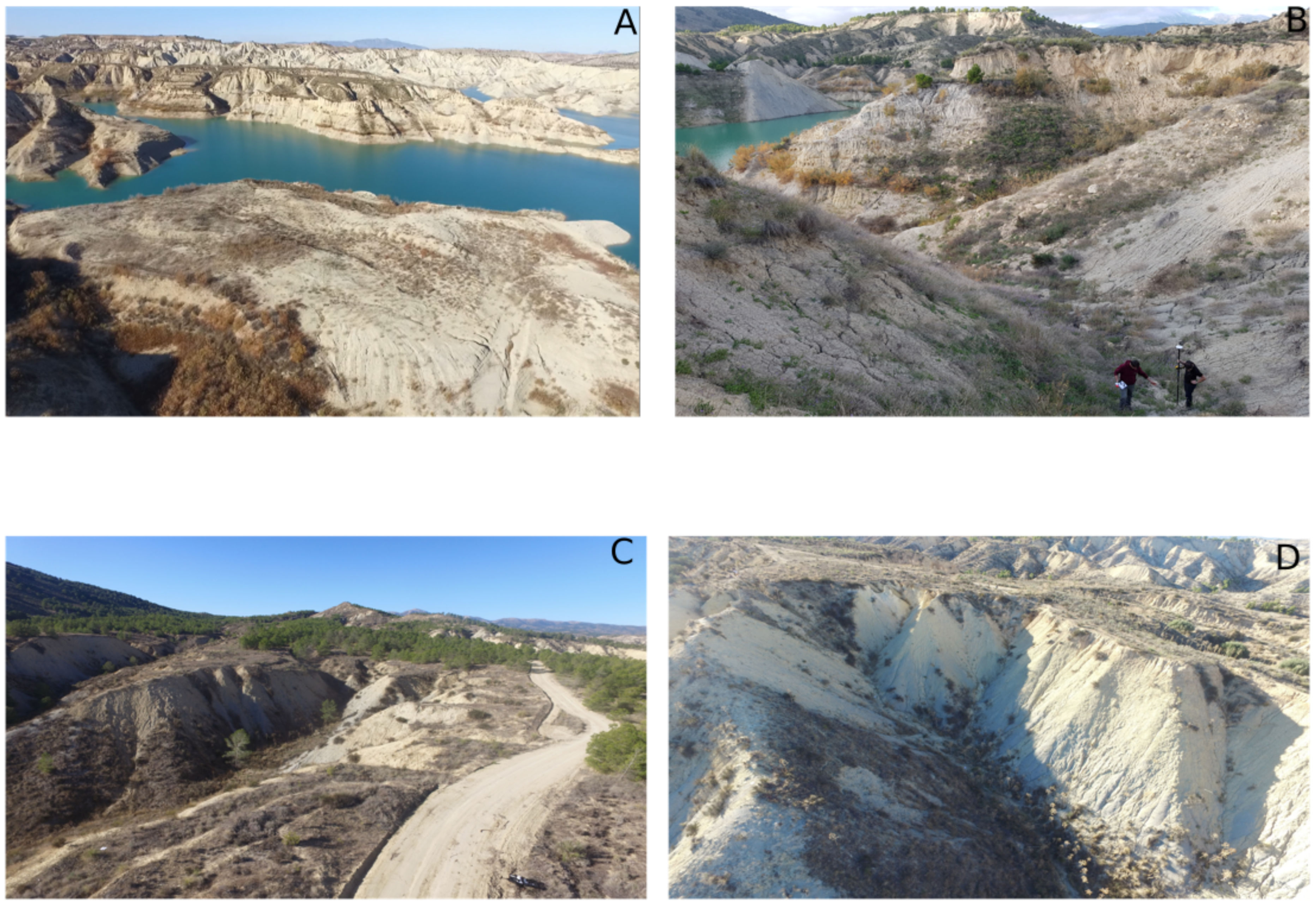
The choice of gullies aimed to represent as faithfully as possible the erosion activity on the lakeshore, in a semi-arid climatic context. This choice takes into account several parameters such as the shape, the exposure, the head of the gullies, the density of the plant cover, and the lithology. Based on the diachronic photo-interpretation of aerial photos (PNOA), three gullies models were selected (
Figure 1).
2.1.1. Site 1
The bank gully (B.G-1) (
Figure 2C), extends over approximately 130 m. It is V-shaped in the upper and middle part, then takes a U-shape downstream from the gully, where the slopes are steep and exposed to the East (low grass cover) or to the West (bare soil). Upstream of the gully (head) is covered by tree layers, planted as part of the restoration project (Proyecto de correccion y repoblacion forestal de las cuencas de las Ramblas de Belen, Librillas y Algeciras. Provincia de Murcia). The North-south oriented gullies have been reforested and are difficult to access. Thus we studied the B.G-1 which is located 250 m from the reservoir. Access to the bank gully of the lakeshore protected by the forest cover and is very difficult. It is for this reason that we chose site B.G-1 which is located at 250 m from the lake.
2.1.2. Site 2
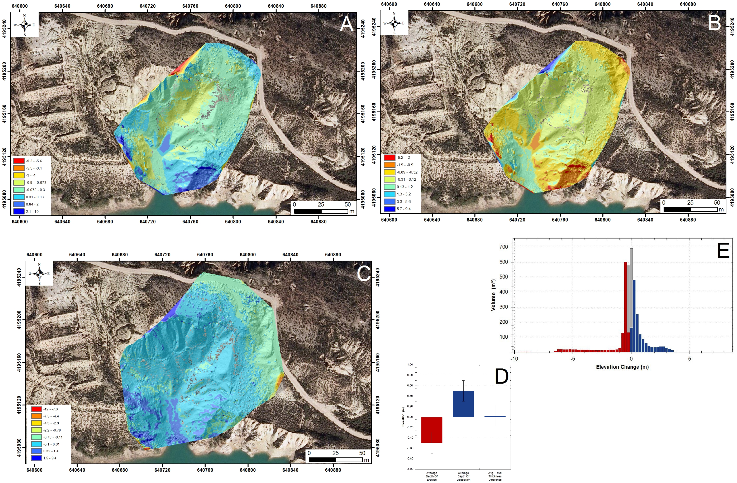
The second bank gully (B.G-2)(B.G-1) (
Figure 2D) is U-shaped. It is oriented East-west with very steep slopes facing North (herbaceous vegetation) and South (bare soil). It is 110 m long, and receives tributary gullies.
2.1.3. Site 3
The third bank gully (B.G-3)(B.G-1) (
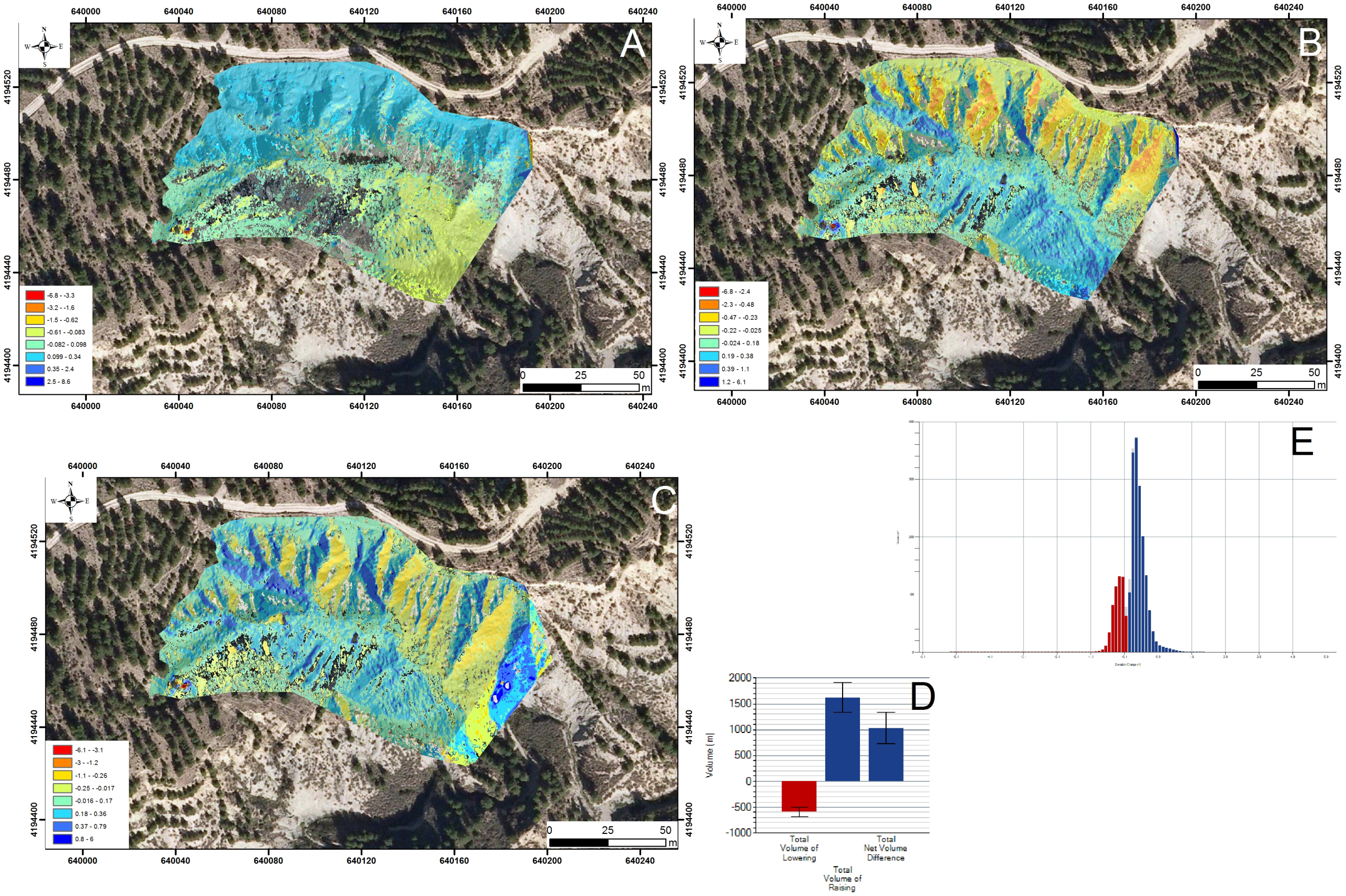
Figure 2B) has a complex shape and is the result of a combination of tunnel gullying (pipig). The slopes of the gully (B.G-3) covered by bare soil. According to photo-interpretation, the B.G-3 gully began to develop after the lake level receded. It’s likely to turn into badlands.
2.2. Precipitation Analysis
2.2.1. Rainfall Extremes
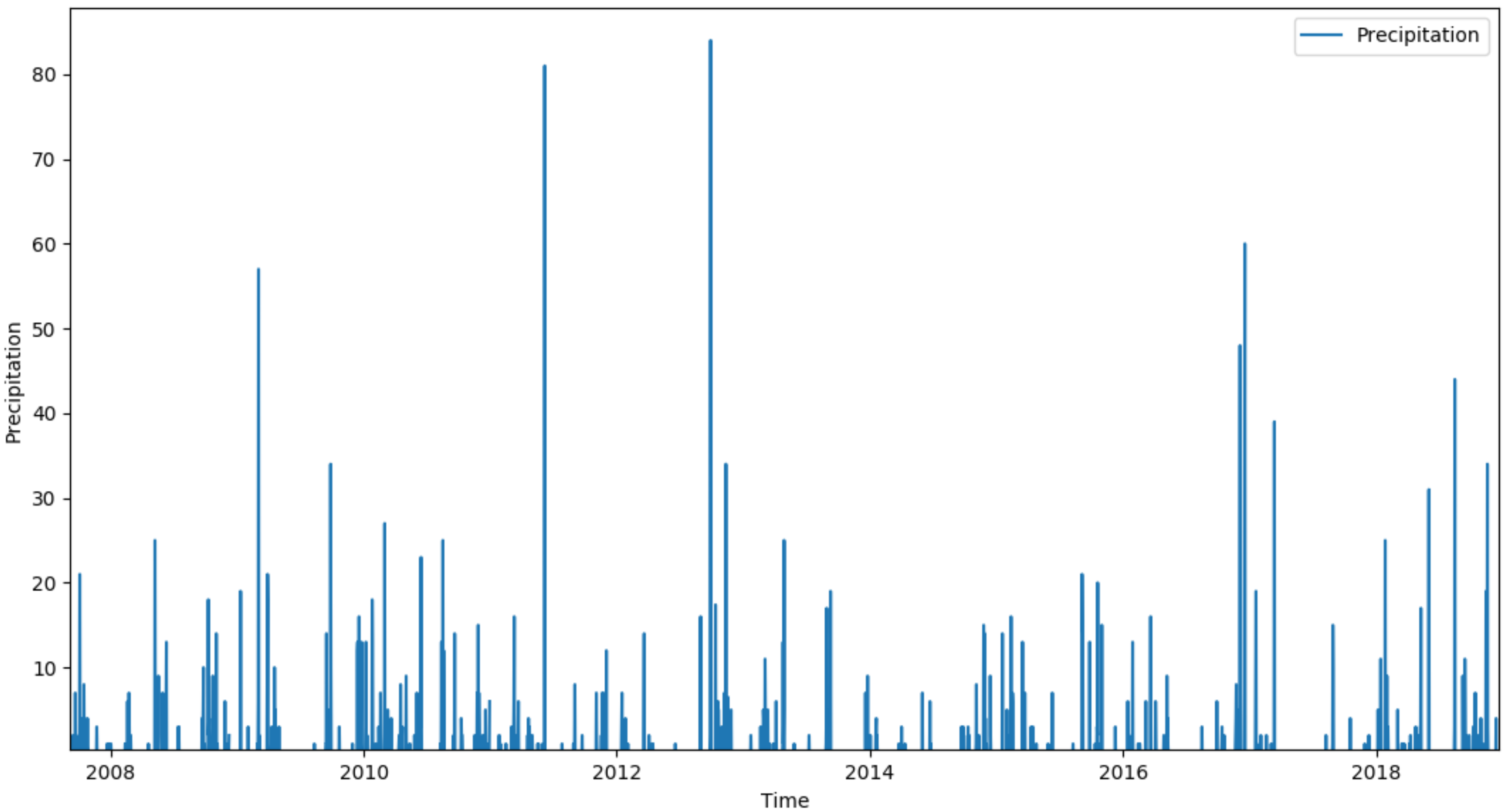
Rare and very rare extreme events were identified using the prec90p index, of the STARDEX project (Statistical and Regional Dynamical downscaling of Extremes for European regions). The prec90p index is used to determine heavy rain events and intense rain when the cumulative daily precipitation values are greater than or equal to 90 and 95 percentiles, respectively. Between 2009 and 2016 there were two heavy showers (
Figure 3).
7 June 2011, with cumulative precipitation of 81 mm in 2 h and a high intensity of precipitation which exceeds 40 mm/h.
28 September 2012, with cumulative precipitation was 84 mm produced in 4 h and an intensity of 21 mm/h.
These two rain events are considered as extreme events and automatically play an important role in erosion. The modification of the precipitation regime with the decrease in the amount of precipitation and rainy days as well as the greater frequency of rare and very rare events during the eight years of topographic surveys can be explained by the effect of climate change in the Mediterranean area [
27].
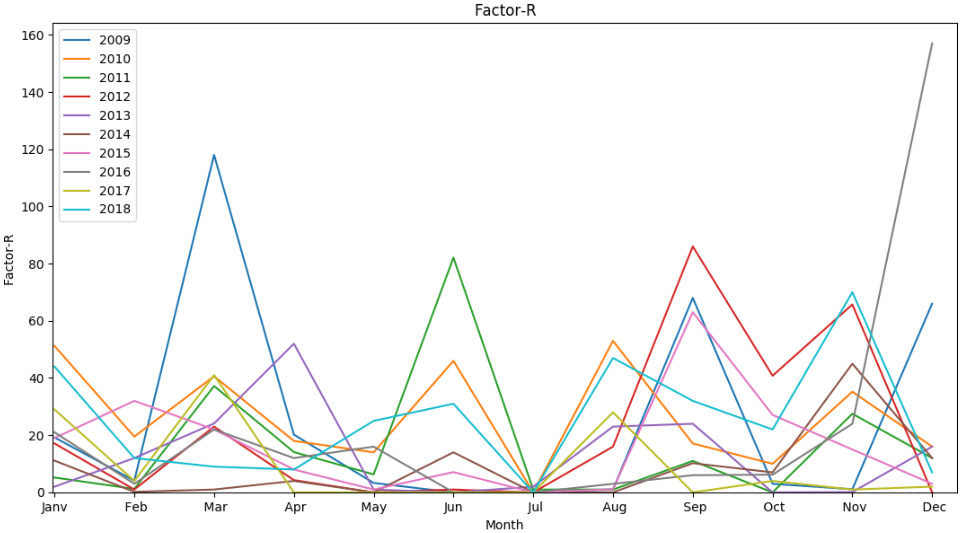
2.2.2. Rainfall Erosivity Factor “R-Factor”
The R-factor was estimated using equation (Equation (
1)) (zone-2) proposed by ICONA for the region of Murcia. The monthly analysis of the factor R traces the evolution of the aggressiveness of the rains on the gullies between the study period of 2009 and 2016 as well as for the year 2018. Between 2009 and 2016 the devastating activity of the rains is concentrated annually in March and September. This activity is linked to the increase in intense rain events during this period. Throughout the period 2009 to 2016, the R-factor peaks are recorded in June 2011 and September 2012, which coincides with an anomaly in the kinetic energy explained by the recording of two extreme phenomena. The year 2018 is relatively wet therefore implying a natural increase in the factor R. From the graph (
Figure 4) we can see that the average value of R, calculated for the wet season, is quite low compared to that of the dry season. During the wet season the values of (R) are moderate with an average of 8.8 MJ cm ha
h
year
, through contribution of the season which recorded an average of 17 MJ cm ha
h
year
. The lowest values are recorded between February and April. Conversely, during the dry season, the highest cumulative value of R is 102 MJ cm ha
h
year
, and it is associated with very intense precipitation in August and November. R: Climate aggressiveness (MJ cm ha
h
year
) PMEX: The maximum monthly value (mm) MR: Cumulative precipitation between October–May (mm) MV: Cumulative precipitation between June–September (mm):
where
R: Rainfall erosivity factor (MJ cm ha h year)
PMEX: Maximum monthly pre-cipitation (mm)
MR: Total rainfall from October to May (mm)
MV: Total rainfall from June–September (mm)
: Ratio of the square of the maximum annual rainfall in 24 hours (mm) to the sum of the maximum monthly rainfall in 24 hours (mm) .
2.3. UAV Data Processing
2.3.1. UAV Data Collection
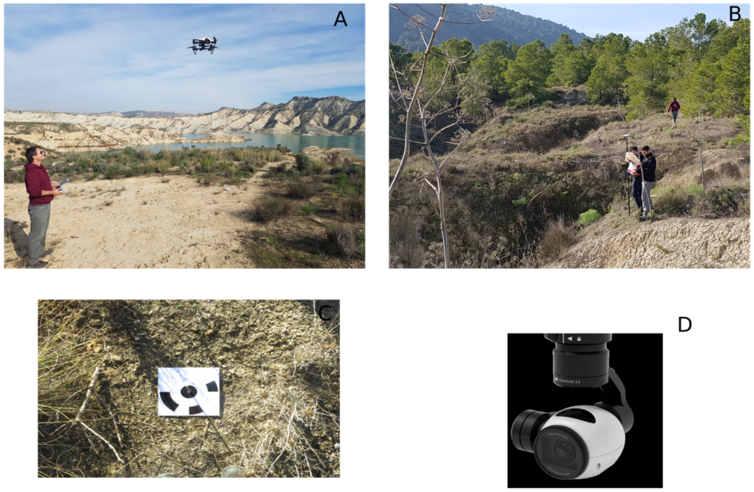
The aerial photography missions were carried out easily and at low cost by the quadriotor drone DJI Inspire 1 v2 (
Figure 5A), equipped with the metric and multispectral camera ZENMUSE X3 without distortion or aspect and with a focal distance of 20 mm (
Figure 5D). The DJI Inspire1 V2 is sold “Ready-To-Fly”, and is designed to have a maximum speed of 22 m/s (ATTI mode, no wind), and a maximum flight time of approximately 18 min. It can reach 2500 m altitude in flight. In addition, it is equipped with a satellite positioning system which uses GLONASS and GPS system.
Flight mission planning was done in navigation mode via the Pix4Dcapture mobile application. After the definition of some flight parameters (flight plan, flight altitude, recovery rate, shooting angle, starting and arrival point of the UAV) the application automatically pilots the UAV. The acquisitions of aerial photos by drone were carried out according to two configurations, for the two gullies (B.G 1 and 2) the photos were taken nadir acquisitions. However, by geomorphological constraints of having gully (B.G-3) we combined the two modes of acquisition nadir and oblique at (30
) in order to model in 3D the overhanging areas of the gully (B.G-3). To ensure a successful photographic reconstruction we have chosen a longitudinal overlap of 80% and a lateral overlap of 60% to avoid gaps between the different photographs. A minimum of 10 ground control points (GCPs) (
Figure 5C) (
Table 1) is required on each site in the middle and at the stable edge, and the same targets were used in each drone mission (except for those which were covered by the sediments), in order to obtain optimal results. The surveys were carried out by the GPS Trimble Geo 7x (
Figure 5B), which includes the following parameters: the ellipsoid GRS 1980, the datum: European Terrestrial Reference System 1989, coordinate system: ETRS89 / UTM zone 30N, with a horizontal accuracy of 1 cm + 1 ppm, and vertical of 1.5 cm + 2 ppm. We used the Stop&Go kinematic approach for the collection of GCPs points. We then made subsequent corrections using RINEX data from a reference station located 30 km from our study area.
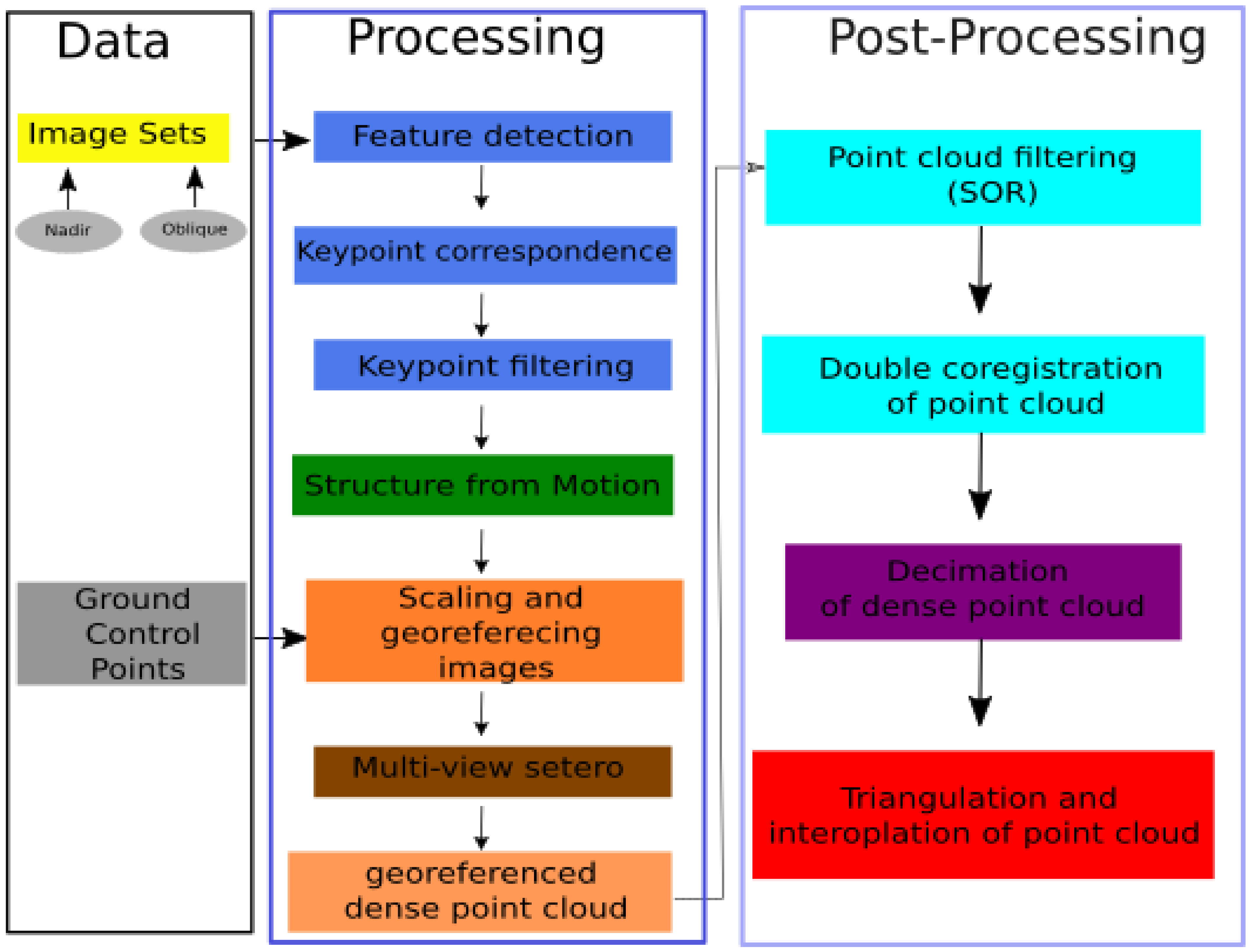
2.3.2. Processing
The aerial photo processing is based on the SfM-MVS photogrammetry technique. We have chosen the Agisoft PhotoScan commercial software to process all the photos taken by the drone, eventually generating dense point clouds and orthomosaics. This software generates exportable datasets and thus has the most comprehensive and easy to use workflow compared to other commercial and open source photogrammetry software’s. The following steps on PhotoScan consisted of establishing dense point clouds which we will then export in ASCII or PTS “XYZ RGB” format (
Figure 6).
2.3.3. Post-Processing
Filtering and Coregistration of Data
CloudCompare open source software is designed for processing and comparing 3D point clouds.The dense 3D point clouds obtained were imported in ASCII XYZRGB formats into the CloudCompare software. We then filtered the point clouds using the SOR filter. Once the point clouds were filtered, we applied the ICP coregistration algorithm to match the homologous points of the multi-temporal point clouds, so that each dense point cloud would refer to the same area [
28,
29,
30,
31,
32].
The Decimation and Interpolation of Point Clouds
Generating a digital terrain model from dense point clouds directly derived from MVS algorithms often requires large computing resources. The interpolation of the points for this kind of processing drains the machines in terms of memory, hence the interest for the decimation of the clouds of dense points which has the potential to reduce the number of points while preserving the topographic complexity of the soil surface. Persistent in the point cloud, we used the ToPCAT geospatial toolbox (Topographic Point Cloud Analysis Toolkit). ToPCAT is an intelligent analysis and decimation algorithm that breaks down the very dense point cloud into a set of non-overlapping meshes, suitable for detecting morphological changes. It then calculates the minimum elevation (
) of each mesh. (
) is considered to be the elevation of bare ground points [
33,
34,
35,
36]. The (
) elevation obtained was then converted to TIN (Triangular Irregular Networks) in order to generate the digital terrain model under the SAGA GIS software.
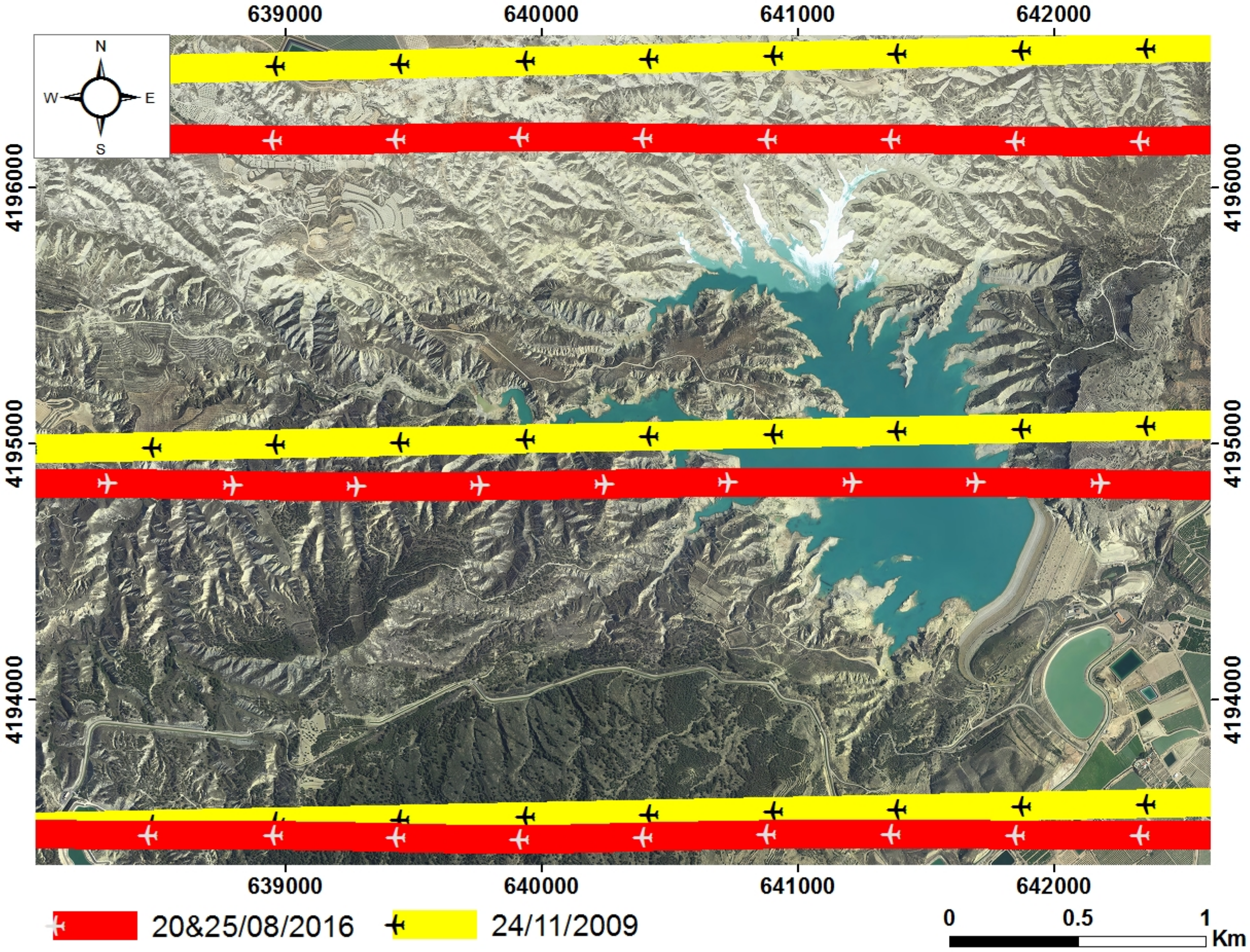
2.4. LiDAR-PNOA Data Processing
In the Murcia region, two ALS airborne LiDAR missions were conducted, on 24 November 2009 and between 20 and 25 August 2016 (
Figure 7). During the first mission, data were collected using a Leica ALS50-II sensor, and for the second mission, data were collected using a Leica ALS60-II sensor.
The LAZ files (binary file compression format LAS version 1.1) that we used come from the ETRS89 UTM Zone 30 geodetic reference system for X, Y and Z coordinates in the EGM08-REDNAP system. Before the classification of the LiDAR point cloud, we prepared the LiDAR raw data in the open source software LASTools. We first converted the LAZ files into LAS files using the las2las algorithm, then we applied a vertical and a horizontal alignment between the flight lines using the lasoverlap algorithm, and finally we transformed the point cloud into EGM08-REDNAP orthometric coordinates using the ascii file <EGM08-REDNAP.asc > and the lasheight algorithm.
Subsequently, we removed outliers and noise using the SOR filter in the CloudCompare software. After pre-processing the point cloud, we chose the MCC-LiDAR v2.15 (Multiscale Curvature Classification) application, an open source command line tool for processing LiDAR data. It classifies data points as ground or non-ground, using the MCC algorithm, to obtain a digital model of bare terrain. Due to the low density of PNOA LiDAR point clouds ranging from 0.5 to 1 point/m, we did not apply a mesh to the cloud.
Finally, the ground points were triangulated and then interpolated with the linear interpolation algorithm under the SAGA GIS software, in order to obtain two ground DTMs of 1 m resolution for 2009 and 2016.
2.4.1. Error Modeling
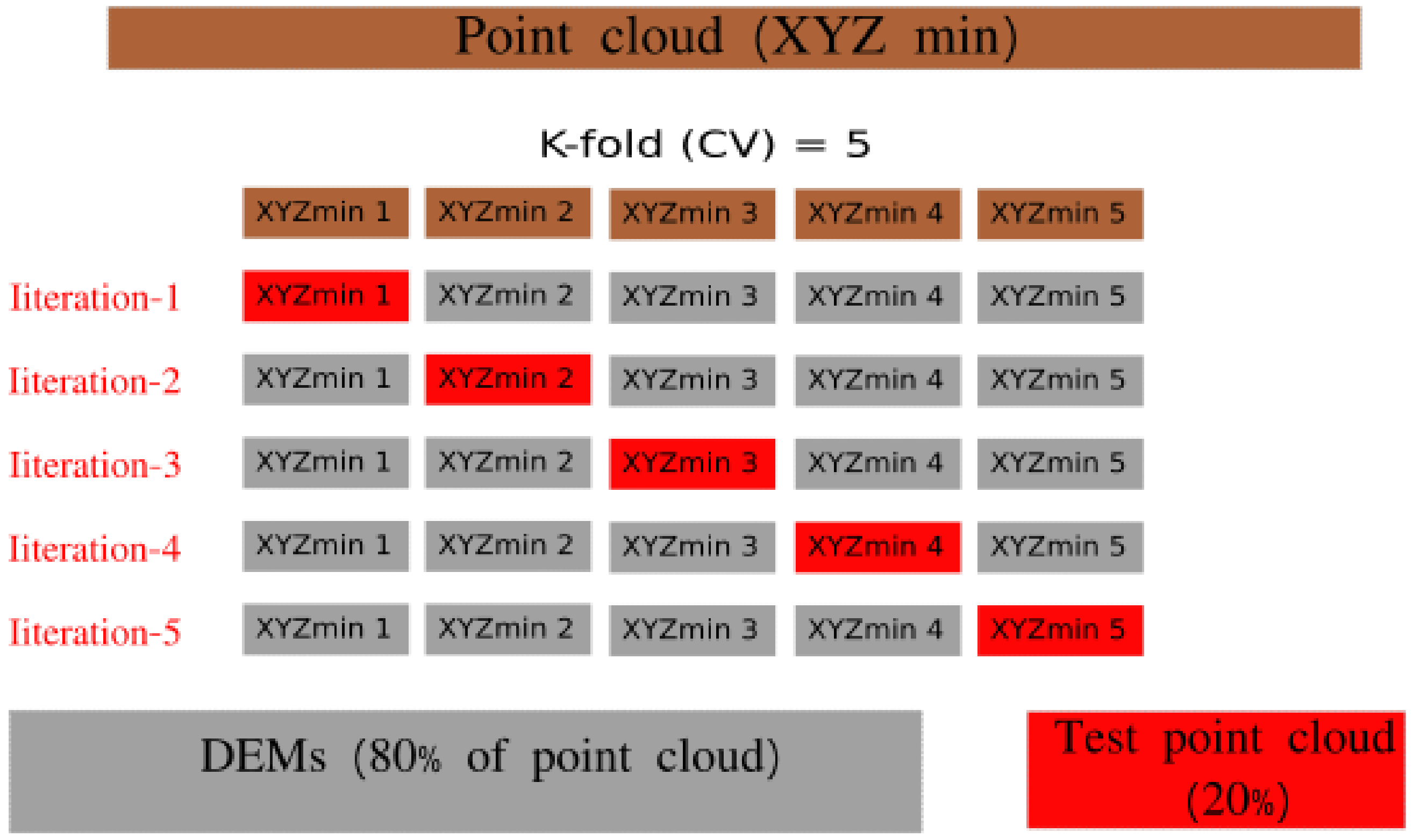
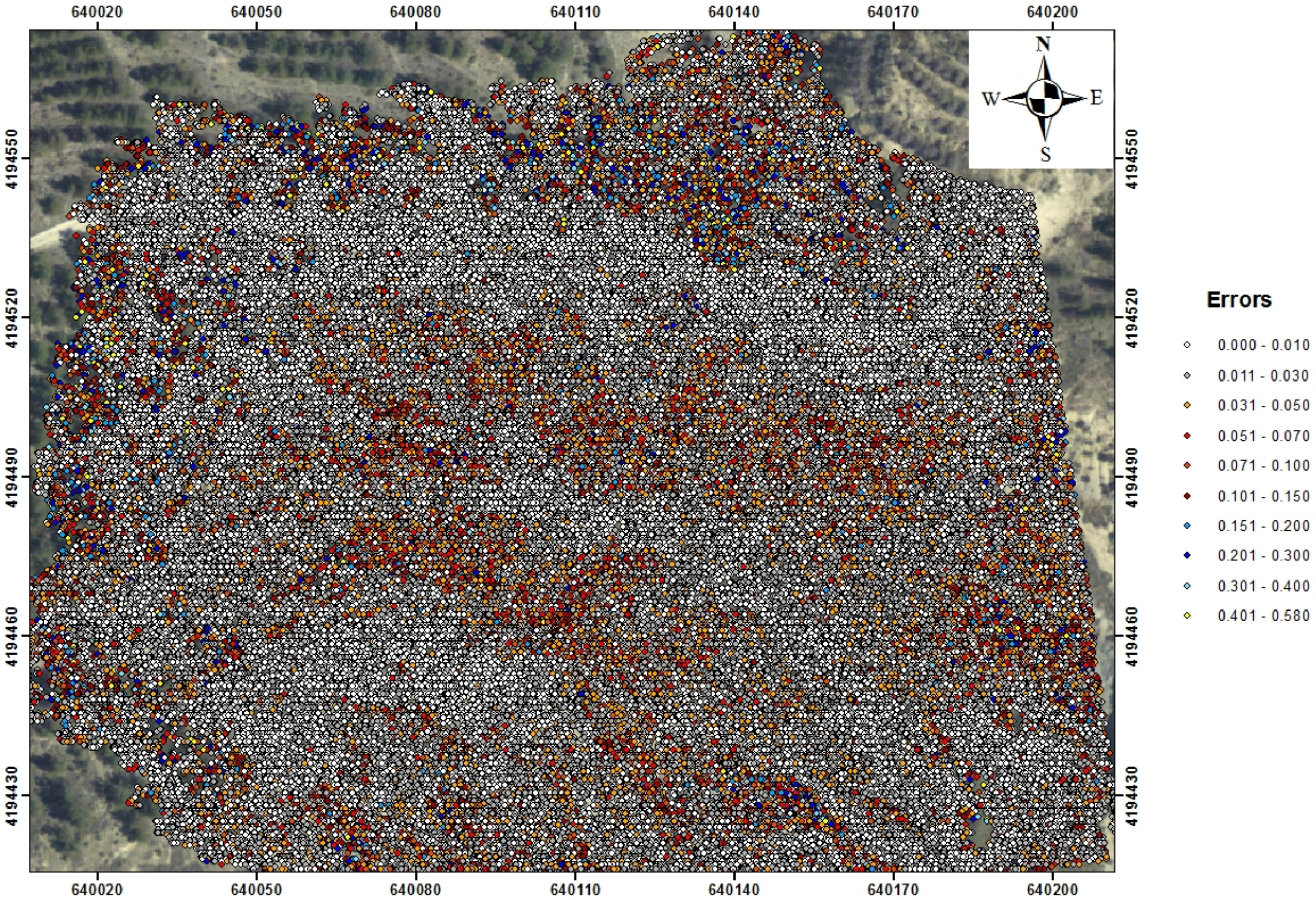
Cross Validation: K-fold Cross-Validation
It is likely that the roughness-based estimates are incorrect, For quantify spatially variable SfM-DEM uncertainty we used cross-validation, then the results of this technique will be integrated from a FIS error model more representative of the different sources of uncertainty. This statistical technique of resampling without replacement consists in dividing the decimated point cloud into validation (20%) and training data (80%) (
Figure 8). The clouds are divided repeatedly with the k-folds (k-fold cross validation) algorithm with a k = 5 (5 subsets of validation point cloud). The training points are interpolated to build a DEM, which compared the validation points in order to quantify the uncertainty of DEM-SfM. We chose the Scikit-Learn (v-0.22.0) free software machine learning library to apply k-fold cross validation on the point cloud decimated by the ToPCAT algorithm. 80% of the (
) points were randomly selected to generate a DEM with a resolution of 5 cm. Then we used the remaining 20% of (
) to compare them with the DEM. The average absolute difference is taken as an indicator of the altimetric uncertainty of the data. The cross-validation test was repeated five times to check the consistency of the results.
Fuzzy Inference System (FIS)
Within the SfM-MVS data, the sources of error vary according to the type of site. In the case of bank gullies, the main sources of error are roughness, slope of the terrain, camera geometry, interpolation error and point cloud density. In this case we were interested in a more comprehensive error modeling that takes into account the different sources of uncertainty. To meet the modelling requirements we adopted a spatially variable FIS (Fuzzy Inference System) error model, which is more reliable model errors in the SfM-MVS-4D data [
35,
37].
We defined four variables as the error sources of the SfM-MVS data to model with the FIS, namely slope, point density, interpolation error, and 3D point cloud error.Slope is the parameter most representative of the topographic complexity of the terrain, and it is the easiest parameter to derive from the DTM or point clouds. The slope (degrees) was generated directly from the decimated ‘’ point clouds with a resolution of 5 cm.
The modeling of the bare ground roughness from the value of the standard deviation of the decimated dense point clouds can be considered to take into account the main source of error of the SfM-MVS-4D data. Terrain roughness affects the ability of the SfM-MVS algorithm to reconstruct the dense point cloud, since the error due to roughness depends on the position of the scan, which is never the same for multi-date missions, as well as the nature and occupancy of the terrain. We recall that vegetation is absent on our study gullies. This facilitates the calculation of roughness.
Then we also generated the interpolation error from a simple absolute difference between the altitude of the TIN node and the DTM-SfM . Finally, for the error variable of the 3D point clouds we used the results of cross-validation.
The matrix data of the different variables were reclassified into four classes (’low’, ’medium’, ’high’ and ’extreme’) (
Table 2).
2.5. Geomorphic Change Detection
An error model makes it possible to associate the control measurements made in the field with an accuracy estimate (example standard deviation in X, Y and Z). When applying the SfM-MVS method to create a digital terrain model, the errors generated are related to several factors such as the position and precision of the control points, camera distortions, resolution, number of photos, processing software, topographic complexity, interpolation methods, surface humidity, vegetation, etc., [
38,
39,
40]. Several sources of error also affect the quality of DTMs for LiDAR data. These sources of error include terrain complexity, vegetation, weather, variation in point density, data filtering process and interpolation technique [
41].
2.5.1. DEM of Difference (DoD)
This approach measures the vertical distance between two DEMs, through a simple subtraction between the pixels of these two DEMs according to the Equation (
2). But before calculating the difference between the DEMs, a threshold value must be set for the minLOD (Equation (
2)) [
42,
43]. This threshold means that substraction values lower than minLoD are revealed as being uncertainties of the two numerical models. We can thus assign a value for the minLoD with confidence intervals that we can set. The user must define this threshold (statistic) according to the probability that he wishes to have so that the detection of changes can be real (Equation (
2)) [
44]. This fast method allows to determine the uncertainties related to the roughness of the terrain, the quality of the point clouds and the acquisition of the point clouds. However, great uncertainty in the quantification of sediment budgets occurs when the DEMs are not precise (since the minLoD threshold will be higher).
where
= The individual error of pixel i of first DTM
= The individual error of pixel i of second DTM
t = is the critical value for a given confidence interval (1.28 for 80% CI, 1.96 for 95% CI); and and are the elevations in a given cell of DEMs.
2.5.2. Multi-scale Model to Model Cloud Comparison-Precision Maps (M3C2-PM)
M3C2-PM is an integrated approach in the CloudCompare software. It is used to directly compare dense point clouds in 3D instead of comparing DTMs or Mesh. The technique calculates the distance in the best perpendicular direction to the surface, with a confidence interval normally set at 95% (to assess the statistical significance of small topographic changes) and a measurement accuracy estimated from the point cloud roughness, allowing us to detect real topographic changes in elevation and planimetry between two degraded surfaces by gullying (erosion or sedimentation). The combination of three factors makes this the preferred method for determining the uncertainty of our digital terrain models: It can work perfectly even with changes in point density and even in the case of missing data. It calculates the distance between point clouds along the normal direction of the surface (the calculation of uncertainty on quasi-vertical areas). It estimates a spatially variable uncertainty for each point cloud and in accordance with terrain roughness and coregistration error [
31,
45]. To apply the M3C2 method, two parameters must be defined:
’D’: Scale and orientation of the normal are used to calculate the normal area of each point which depends on the roughness and geometry of the point clouds. In the case of bank gullies we first applied a local model of <Quadric >shape along the preferential axis to orient the reference point cloud towards the comparison point cloud. Then we chose the value of D/2 = 10 cm to look for neighbouring points in the reference point cloud while taking into account the terrain roughness.
’d’: Projection scale, or the diameter of the cylinder in which the average distance of each surface of the point clouds is calculated. In this study we used a value of d = 20cm.
4. Discussion
4.1. Data Acquisition
The acquisitions of SfM-MVS-4D data by UAV met our needs in terms of accuracy, and frequency of monitoring the gullies along the lakeshore. Throughout the shooting, the flight altitude remained at a quasi-constant level at each site during the three missions, allowing us to keep the same pixel resolution for each gully. The UAV flew over the gullies at an altitude varying between 28 and 37 m, which allowed us to guarantee adequate resolution for monitoring topographic changes in the gullies. We also noted that the choice of these altitudes allowed us to ensure a small B/h ratio of the order of 0.6, in order to minimize as much as possible the surface of the hidden areas.
The results of the dense point clouds obtained by a vertical shot provide significant information on the topography of the gullies (B.G-1 & 2) compared to the gully (B.G-3). However, it should be noted that the photos taken on the gully (B.G-3) with a vertical camera do not cover the entire studied area. The overhang, having a vertical geometry, could not be taken into consideration. Moreover, the photos taken with an oblique camera were very useful to link the base and the top of the gully overhang slopes. Several previous studies have shown that the systematic errors of the dome effect significantly decrease or even eliminate after the use of an oblique and nadir image acquisition configuration, regardless of the image overlap rate, the camera angle and the configuration of the oblique and nadir images [
46,
47]. On the gullies (B.G-1 and B.G-2) the aerial photos are taken at nadir. The application of the integrated approach of the two flight configurations, i.e. nadir (90
) and oblique (30
) acquisition, reinforces the geometry of the photo network on the gully (B.G-3). This technique of oblique photo acquisition increases the overlap rate between the photos, making it possible on the one hand to densify the density of the point clouds and on the other hand to fill the void created by the topographical complexity of the gullies (overhang). This therefore reduces georeferencing errors linked mainly to the low precision of the GCPs. We noted that the integrated approach has considerably reduced the RMSE in XYZ of the GCPs on the gully (B.G-3) with an average that does not exceed 1.4 cm in X, 1.2 cm in Y and 1.3 cm in Z during the three missions, bearing in mind that the GCPs went from 16 points to 12 points during the last mission. For the gullies (B.G-1; 2) it is the opposite, since the RMSE errors are high and vary between 2 and 5 cm.
4.2. Data Processing
Vertical and oblique photos are somewhat contrasting since the angle between the two shooting modes fluctuates very strongly along the same swath. Alignment in the PhotoScan software of the photos from two angles failed. The alignment results of the two shooting modes contain only the sparse point cloud from the nadir photos. To solve this problem we realigned all the photos using the common GCPs on both photos and the geolocation data of the photos before applying the bundle adjustment model.
Then we included the following camera parameters: Fit F, Cx, Cy, K1, K2, K3, P1, P2 (
Table 4) which improved the camera model and reduced the RMSE errors of the photos as well as the deviations at the GCP point networks. The parameters were selected based on correlation analysis where high correlation parameters were eliminated to avoid over-configuration of the camera model. In this case study Mean precision across the camera is 0.10, this precision value will allow us to evaluate the correlation between the camera parameters. The low correlation between the parameters indicates a good image network except for the radial parameters, however when the correlation between F and Cy is very high this is explained by the absence of large camera rotation and a slight weakness of the image network. In our case study, the value is very close to the accuracy which illustrates the good image network taken in the field.
4.3. Error Modeling
We took advantage of the Lidar PNOA data collected between 2009 and 2016 to continue the analysis of the morpho-sedimentary dynamics of the three gullies. Similarly, the work was enriched by taking into account the spatio-temporal variability of the dynamics of all the bank gullies as a function of topographical influence and climate action. We present and analyze here the results of the raw DoD method obtained from the difference between the two DEMs Lidar 2009 and 2016 of the PNOA project. however, the error of the two Lidar missions PNOA 2009 and 2016 is of the order of 0.28 m this value is considered spatially homogeneous and uniform for two main reasons:
(1) The low density of the Lidar point clouds (between 0.5 and 1/m): the denser the point cloud is, the more robust it is to accurately determine terrain parameters such as slope or roughness.
(2) The absence of GCPs: the georeferencing errors of the GCPs are essential to estimate an error model of the Lidar PNOA data.
To quantify the uncertainty of the SfM-MVS data accurately, it is necessary to validate the SfM-MVS data by a comparison with previous SfM-MVS data or with a very high precision field truth (DGPS, TS). The method of validation is often dictated by the extent, scale, field survey method, data format, and morphological characteristics of the study site.
In this paper we first chose to quantify spatially variable SfM DEM uncertainty, using the cross-validation method instead of Bootstrapping which has already been used by Wheatonand [
35] and Rossi [
48]. Then the uncertainty values will be used to build an error model that takes into account the different sources of uncertainty using the FIS model.
Several works have shown that the vertical accuracy on the GCPs control points is about two to three times higher than the accuracy obtained by the products derived from the SfM-MVS data (DTM and orthophotography) [
49,
50]. The table (
Table 5) shows that the FIS error propagation model estimates higher vertical errors on GCPs points than those obtained after georeferencing (
Table 3). The accuracy of the SfM-MVS data obtained during this study is comparable to that of the GNSS/TS data [
35,
51].
4.4. Detection of Geomorphological Changes
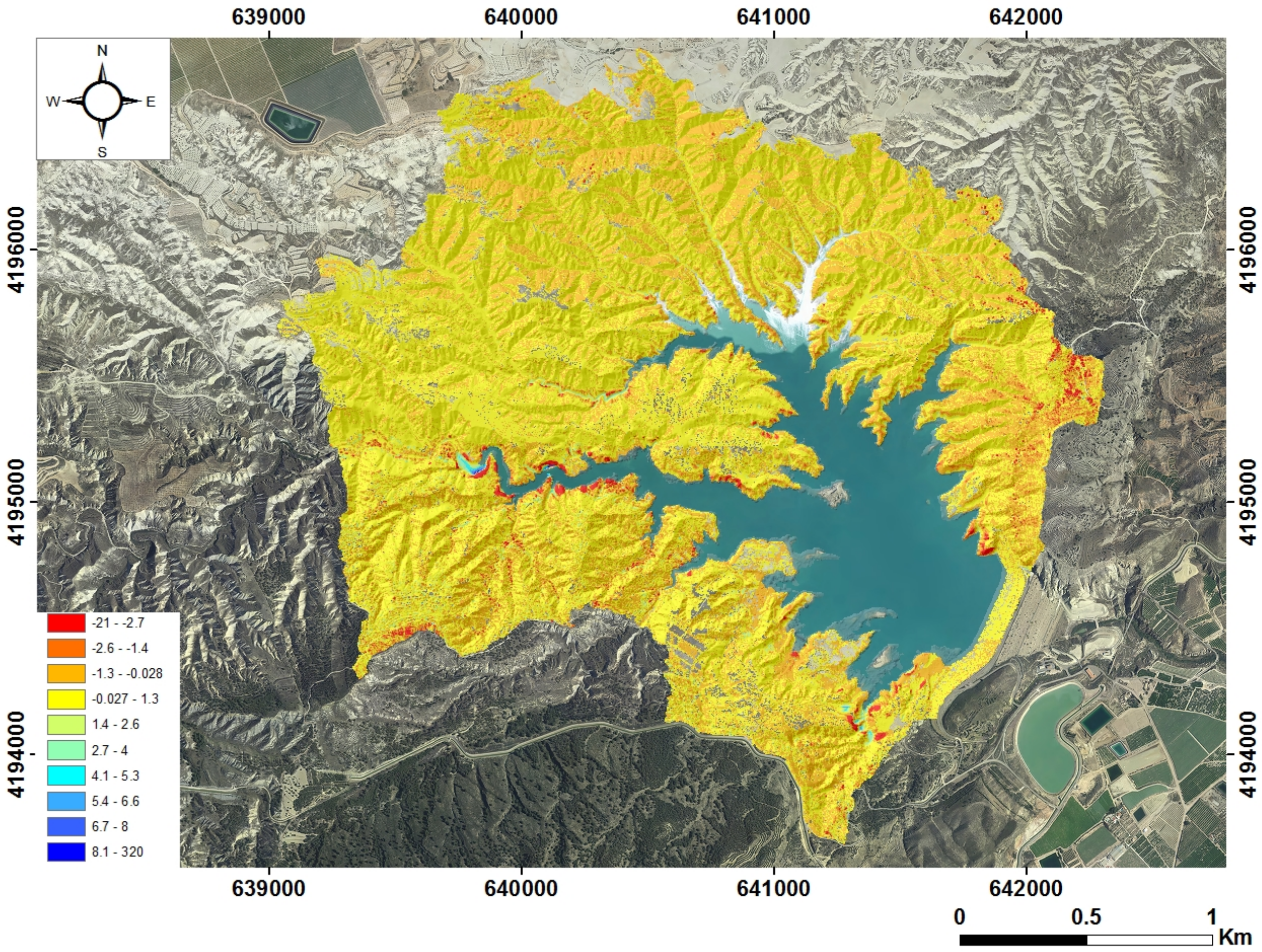
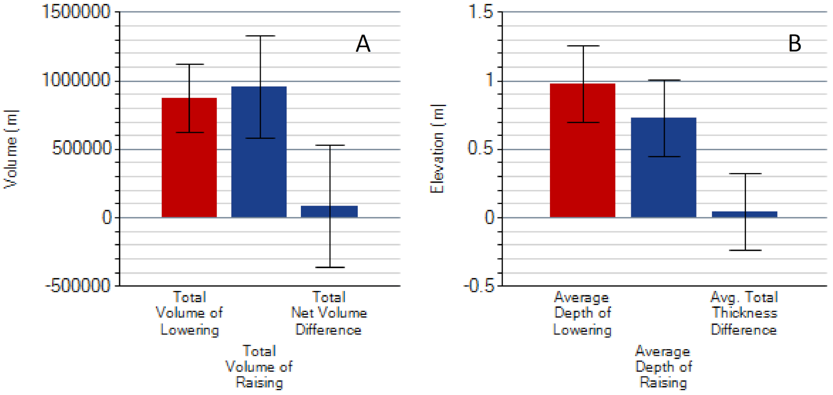
From the
Figure 16 we observe a ramified gully system on the entire lakeshore, with a gully density varying between 18 km/km
and 59 km/km
with an annual erosion rate of 39 T/ha/year these values are extreme are of the same order as some areas that reach values varying between 15% and 60% [
52,
53,
54,
55].
Globally, the volume eroded by gullies varies between 0.002 and 47,430 m
/year with an average of 358.6 m
/year. In the Murcia region, research on the gully erosion is limited. As a result, there is very little data on the gully erosion budget. Indeed, in the literature, we find two references on the sediment balance of gullies and bank gullies in the Guadalentin watershed downstream of the Rambla de Algeciras watershed, namely the work of L. Vandekerckhove [
56] and Marzolff [
57]. Before comparing the results of this study with those of Vandekerckhove and Marzolff, it should be pointed out that the very complex morphology, the very friable pedology and the strong anthropic activity in the Rambla de Algeciras catchment area allowed us to consider that the Guadalentin basin is less vulnerable to gully erosion than the Rambla de Algeciras basin. Despite this observation, the volumes calculated in this work are close to the results estimated in this study. The annual volume calculated by Vandekerckhove over some time varies between 40 and 43 years based on aerial photos and field measurements vary between 13 and 3467 m
/year. Similarly, Marzolff’s work in 2011 using aerial photos taken by the UAV showed that the rate varies between 0.5 and 100 m
/year. On the gully (B.G-3) we have estimated the volume eroded from the calculation of the distance between the 3D SfM-MVS point clouds according to the direction of the surface normals, rather than the difference between two 2.5 D rasters. This technique takes into account the volume of sediments eroded on the gully overhang area. The M3C2 algorithm calculates the distance between the multi-temporal point clouds, which allows to estimate the eroded volume with high accuracy. The results of the M3C2 technique thus testify on the good choice of an oblique and nadir acquisition configuration on the gully (B.G-3) to generate accurate and complete SfM-MVS data.
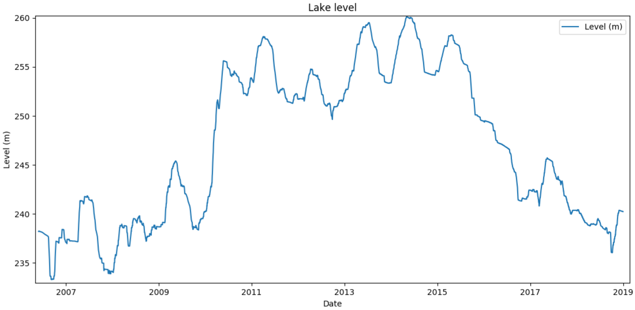
The analysis of the geomorphological changes estimated by the UAV and LiDAR are very different, with the results of the LiDAR data the percentage of the eroded area over the whole period 2009–2016 is not more than (45%) however the deposit areas are more important with a percentage of (55%). On the other hand, the estimates of the sedimentary balance during the year 2018 with the UAV data allow us to observe an erosion activity that affected on average more than 60% of the surface of the studied gullies. The results of the LiDAR data appeared aberrant but the monitoring of the fluctuation of the lake level explains the strong sedimentation activity on the lake banks between 2009 and 2016. The rise of lake level is related to the high trend in rainfall inputs between 2010 and 2015 (
Figure 17). It should also be noted that the lake level decreased from 260 m in 2014 to 240 m in 2018. This is related to the decrease in rainfall inputs between 2015 and 2017. This water level fluctuation has caused the settling of regression deposits. After the period of maximum lake filling at 260.12 m (4 May 2014), the lakeshore has experienced silt sedimentation in flat areas and gully beds. These sediments have four origins:
The photo-interpretation of PNOA orthophotography illustrates an imbalance in the morphodynamics of the lakeshore.
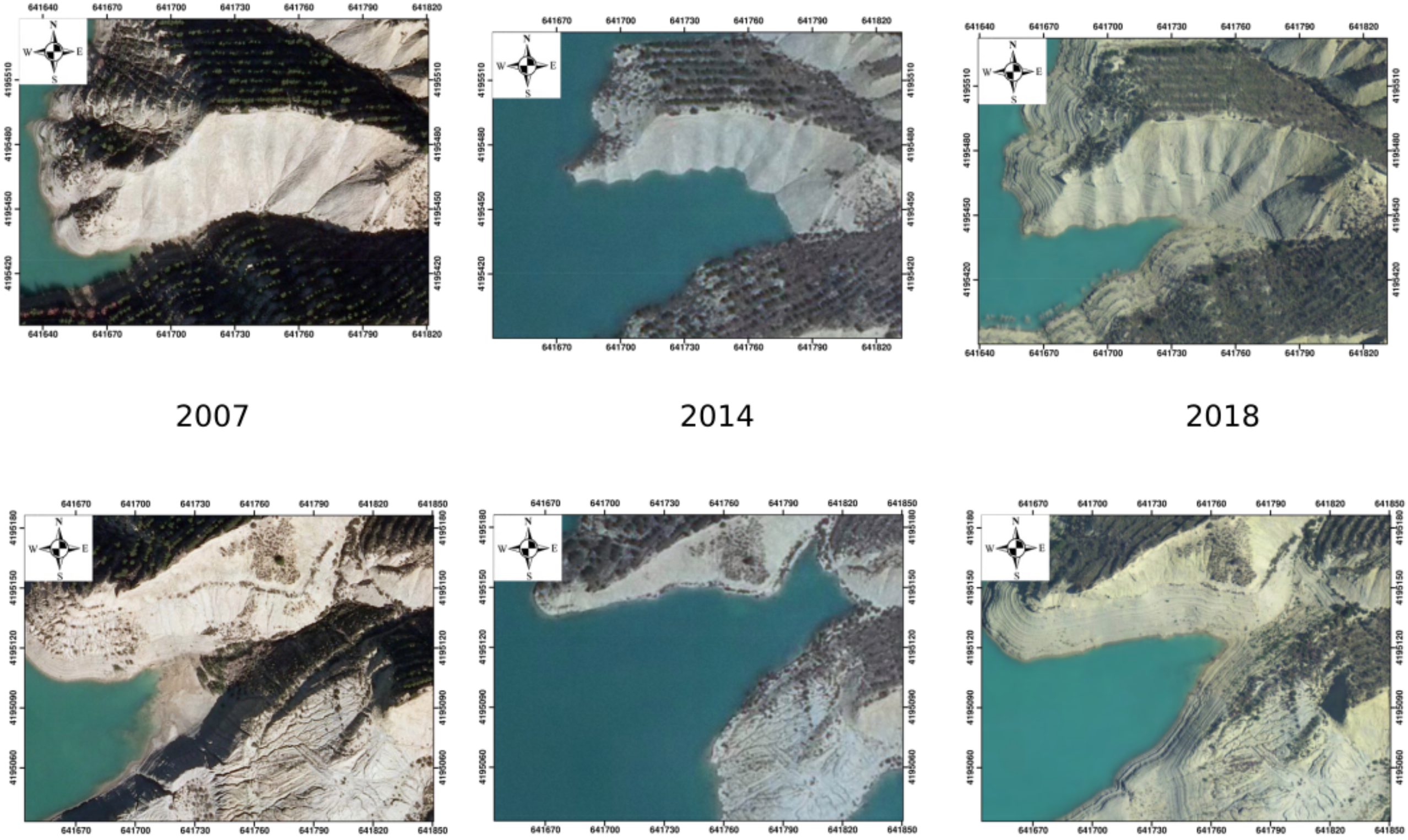
When the lake level reached the rills and small gullies, the vertical movement of the lake water overwhelmed them and caused them to lose their erosion ability (
Figure 18). This has led to the temporal disappearance of these small forms of erosion. They were then replaced by the sedimentary activity of waves loaded with suspended matter (a process linked to longshore drift).
The missing data on the solid transport at gauging stations tributaries of the Rambla, prevent from quantifying the sediment inputs into the Rambla de Algeciras, as it has been done in Morocco by Ezzaouini et al. [
58], and unfortunately also, we have not been able to install sedimentometres [
59] in the lake to collect and analyze the nature and percentage of detrital and biogenic sediments, mainly due to time and money issues.
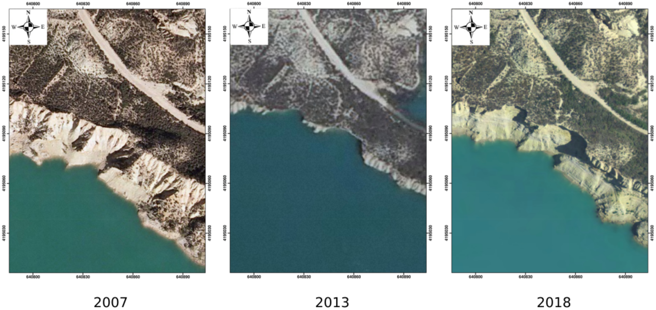
The bluff slumping of the lakeshore, observed through photo-interpretation of the PNOA aerial orthophotographs between 2009 and 2016, is a phenomenon triggered during the maximum filling of the lake. The former overhanging areas are destabilized by moisture and weight. This phenomenon is localized in particular on the meanders and concave banks of the Rambla (
Figure 19).
5. Conclusions
The friable nature of the soil, the fluctuation of the lake level, anthropic activity and climate changes marked by increasingly rare but very violent rainfall episodes have made it possible to carve out several forms of gullies on the lakeshores of Rambla de Algeciras. The main goal of this paper is to demonstrate whether the SfM-MVS-4D model generated from photos taken by a UAV and the LiDAR PNOA data, are able to accurately quantify the sediment budget on the banks gullies of the lakeshores. The answer is yes. Indeed, for bank gully monitoring on lakeshores, we detected geomorphological changes on three types of banks gullies. The models for the detection of geomorphological changes were constructed using multi-temporal numerical terrain models coupled with spatially variable uncertainty models. The rate of geomorphological changes detected on the three gullies in 2018 is mainly related to orientation, land use and the shape of the gullies.
The aerial photos taken by the UAV are capable of generating SfM-MVS-4D models with very high spatial and temporal resolution, which allows to highlight the movement of sediments along the slopes of the gullies. The use of the nadir and oblique configuration for taking pictures has improved the accuracy of the SfM-MVS models taken on very steep slopes or with overhangs. This accuracy was measured using several techniques, namely georeferencing error estimation and the statistical cross-validation approach and finally the FIS technique. This was useful for detecting geomorphological changes on banks gullies. The accuracy of the SfM-MVS data varies between 1 and 5 cm.
The data from the PNOA project (orthophotographs and LiDAR) provided reliable and accurate data to study the effects of lake level fluctuation, climate change and land use change on the initiation of lake bank gullying. The DOD technique applied on the LiDAR data from the PNOA allowed the estimation of an annual sedimentation rate of 39 T/ha/year (49 m/ha/year) from the gullies of the Rambla de Algeciras lakeshores.
We also note that the approach proposed in this paper will be deployed in Morocco on the Sidi Mohamed Ben Abdellah dam, which shares the same bank gully on lakeshores issues and geo-environmental characteristics as our study site.


 ,
, 


