GuEstNBL: The Software for the Guided Estimation of the Natural Background Levels of the Aquifers

 ,
, 

Abstract
1. Introduction
2. Materials and Methods
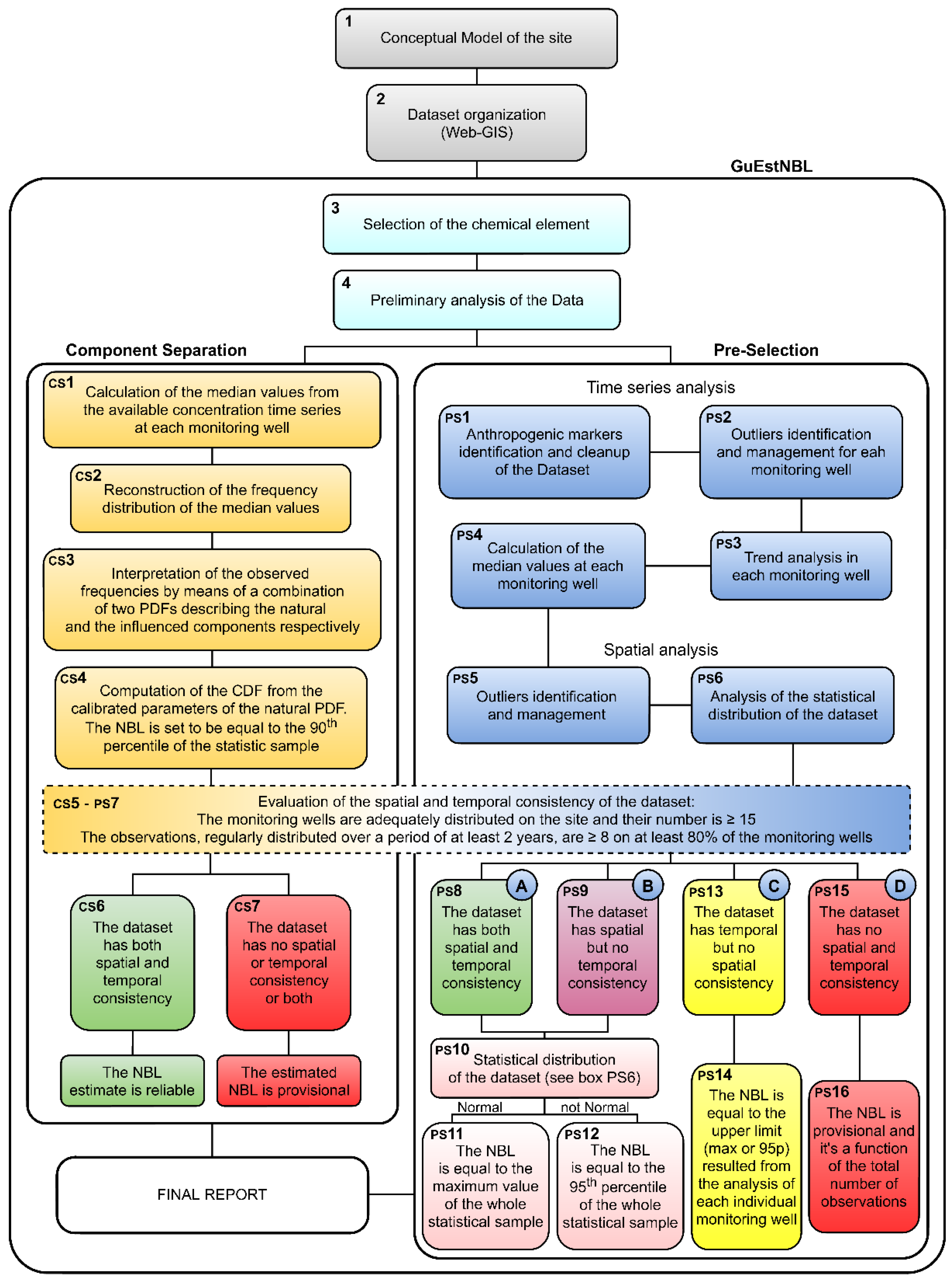
2.1. Structure of the Software-Based NBL Determination Procedure
2.1.1. Data Scheduling and Acquisition
- Block 1 (Conceptual model of the site)
- Block 2 (Dataset organization (Web-GIS))
2.1.2. GuEstNBL
- Block 3 (Selection of the chemical element)
- Block 4 (Preliminary analysis of the data)
2.1.3. Component Separation Method
- Blocks CS1 and CS2 (Calculation of the median values and construction of the observed frequency distribution)
- Block CS3 (Interpretation of the observed frequencies)
- Block CS4 (NBL calculation)
- Blocks CS5-CS7 (NBL reliability)
2.1.4. Pre-Selection Method
- Block PS1 (Dataset Pre-selection)
- Block PS2 (Temporal outlier identification and management)
- Block PS3 (Trend analysis)
- Block PS4 (Calculation of the median values)
- Block PS5 (Spatial outlier identification and management)
- Block PS6 (Analysis of the statistical distribution of the dataset)
- Block PS7 (Spatial and temporal consistency of the dataset)
- Block PS8-PS12 (NBL determination for the datasets falling into cases A and B)
- Block PS13-PS14 (NBL determination for the datasets falling into case C)
- Block PS15-PS16 (NBL determination for the datasets falling into case D)
2.1.5. Final Report
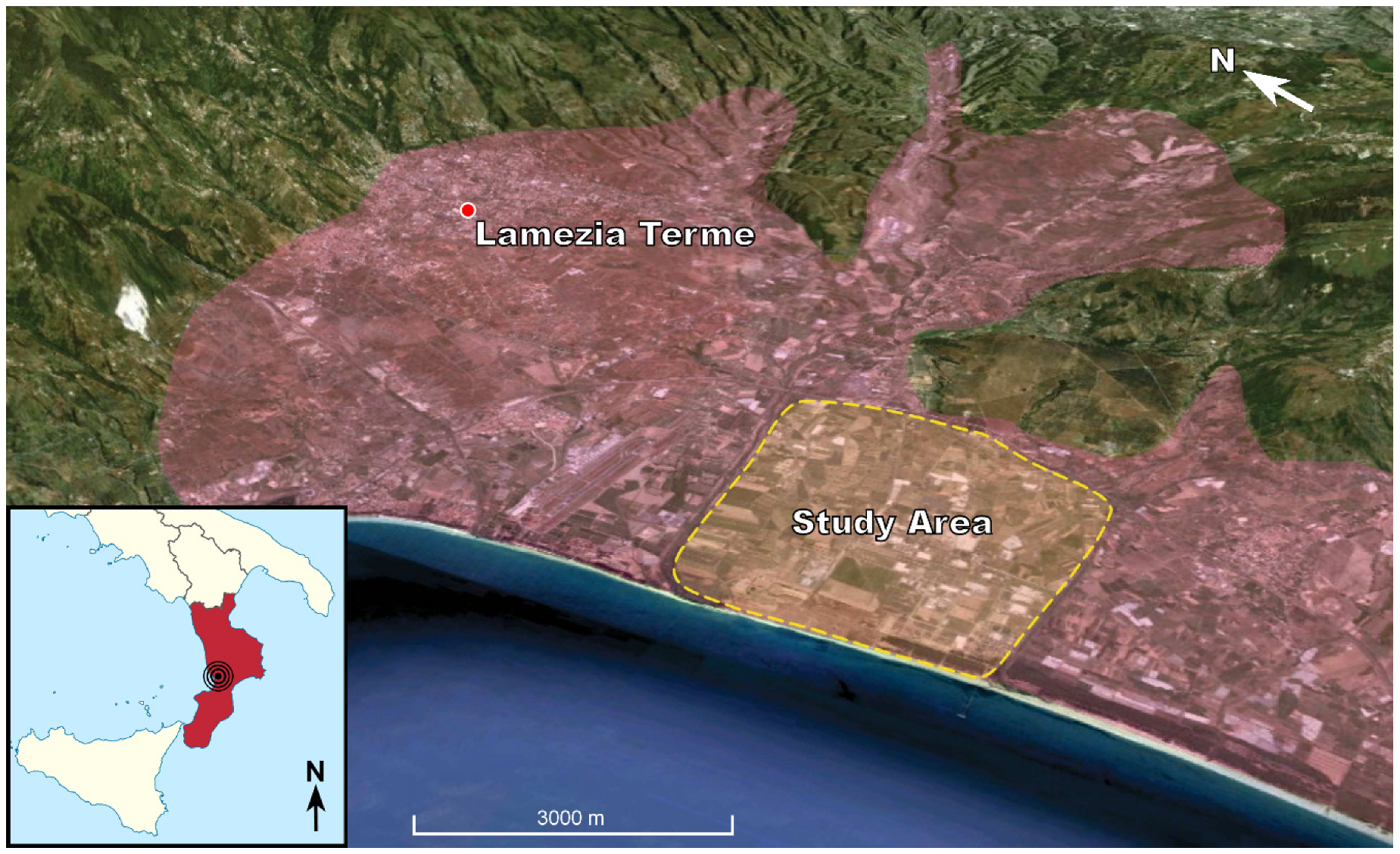
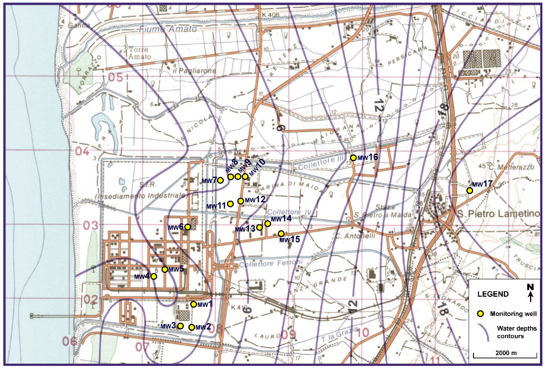
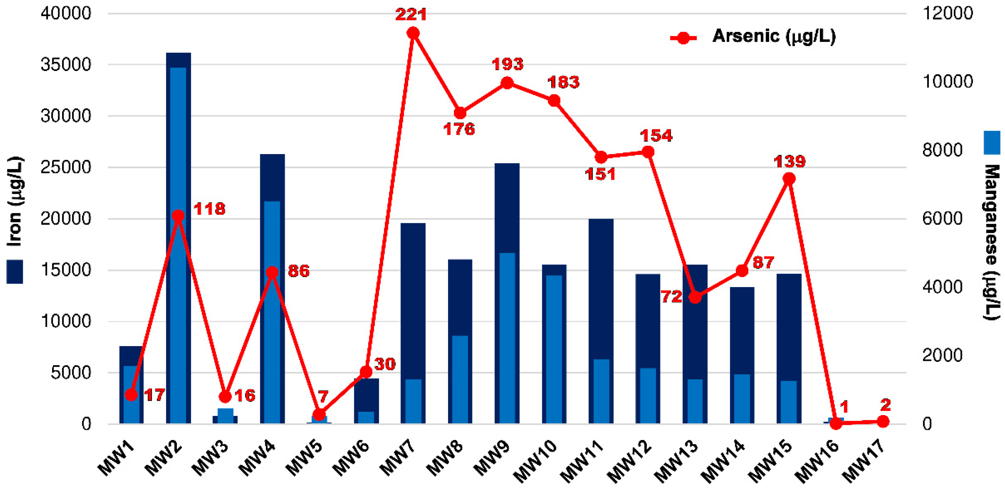
2.2. Study Area
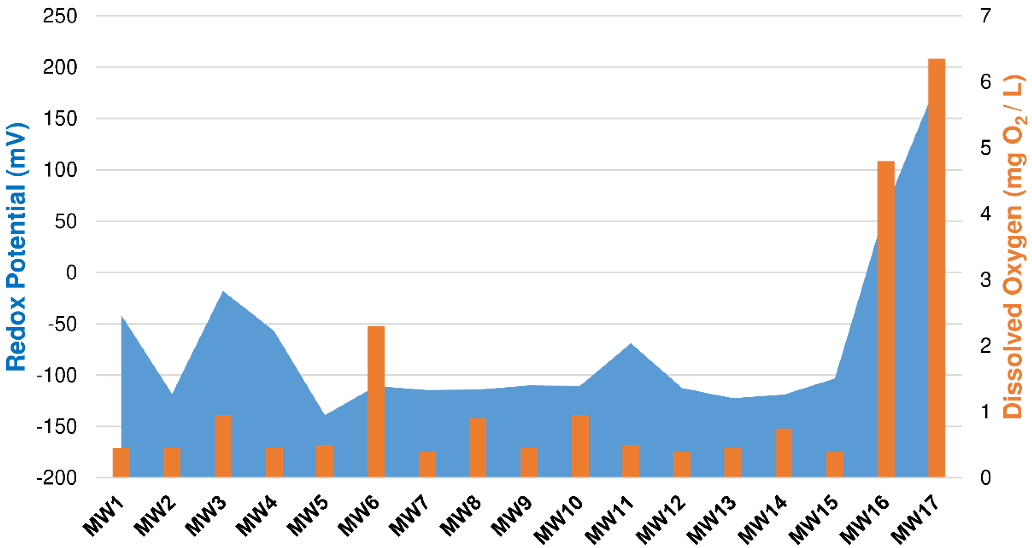
3. Results
3.1. Natural Background Levels Estimation
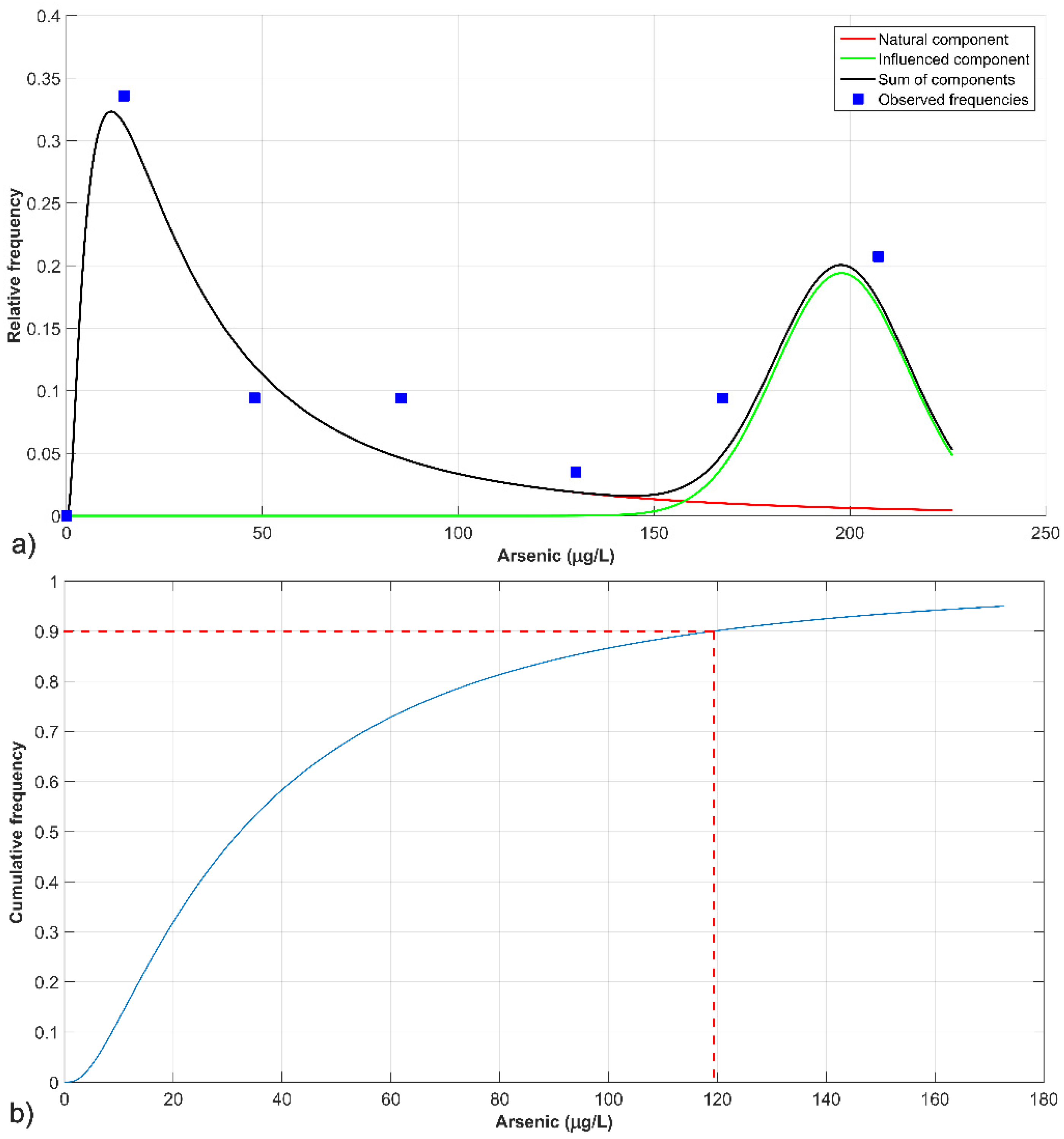
3.1.1. Arsenic
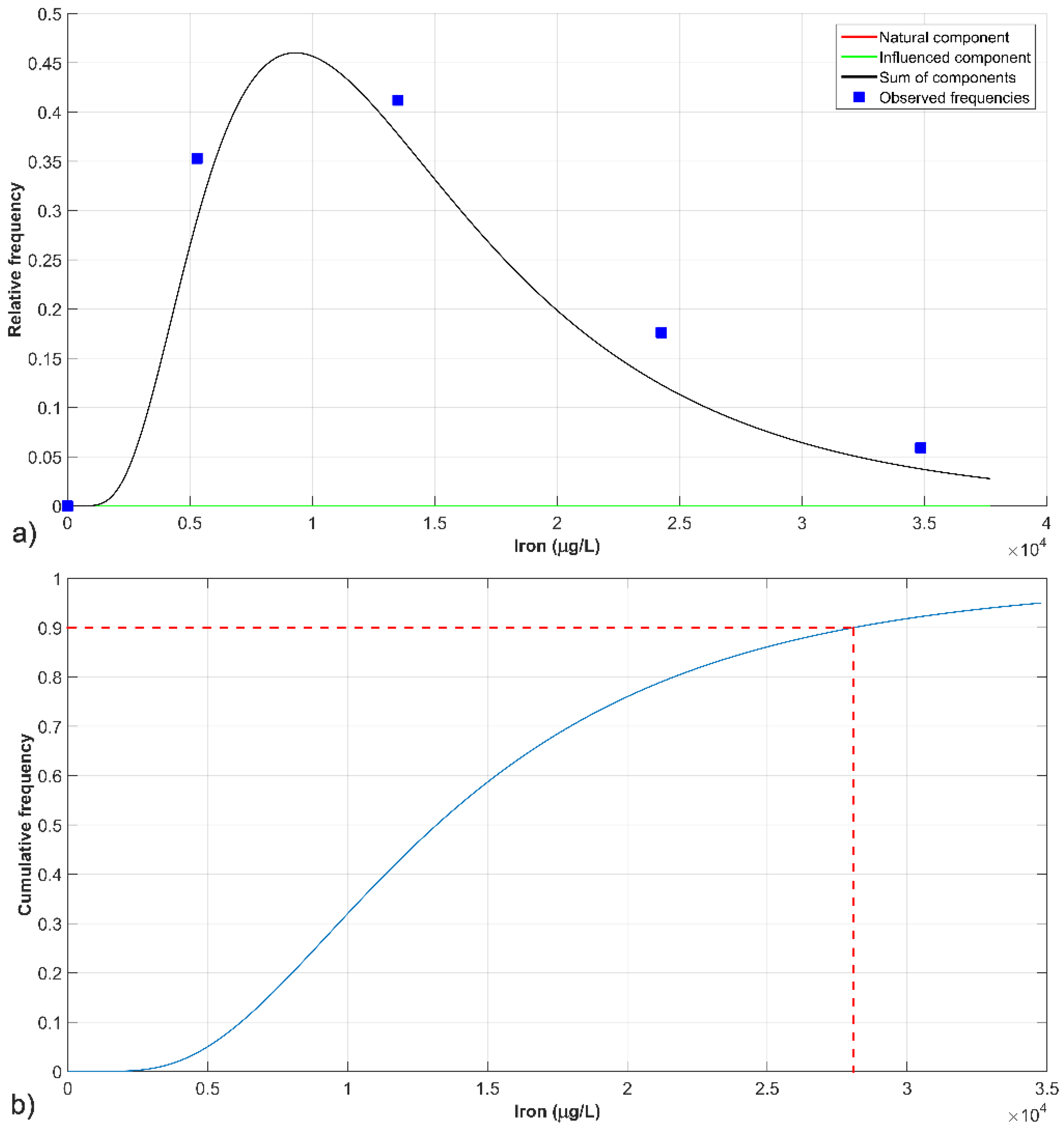
3.1.2. Iron
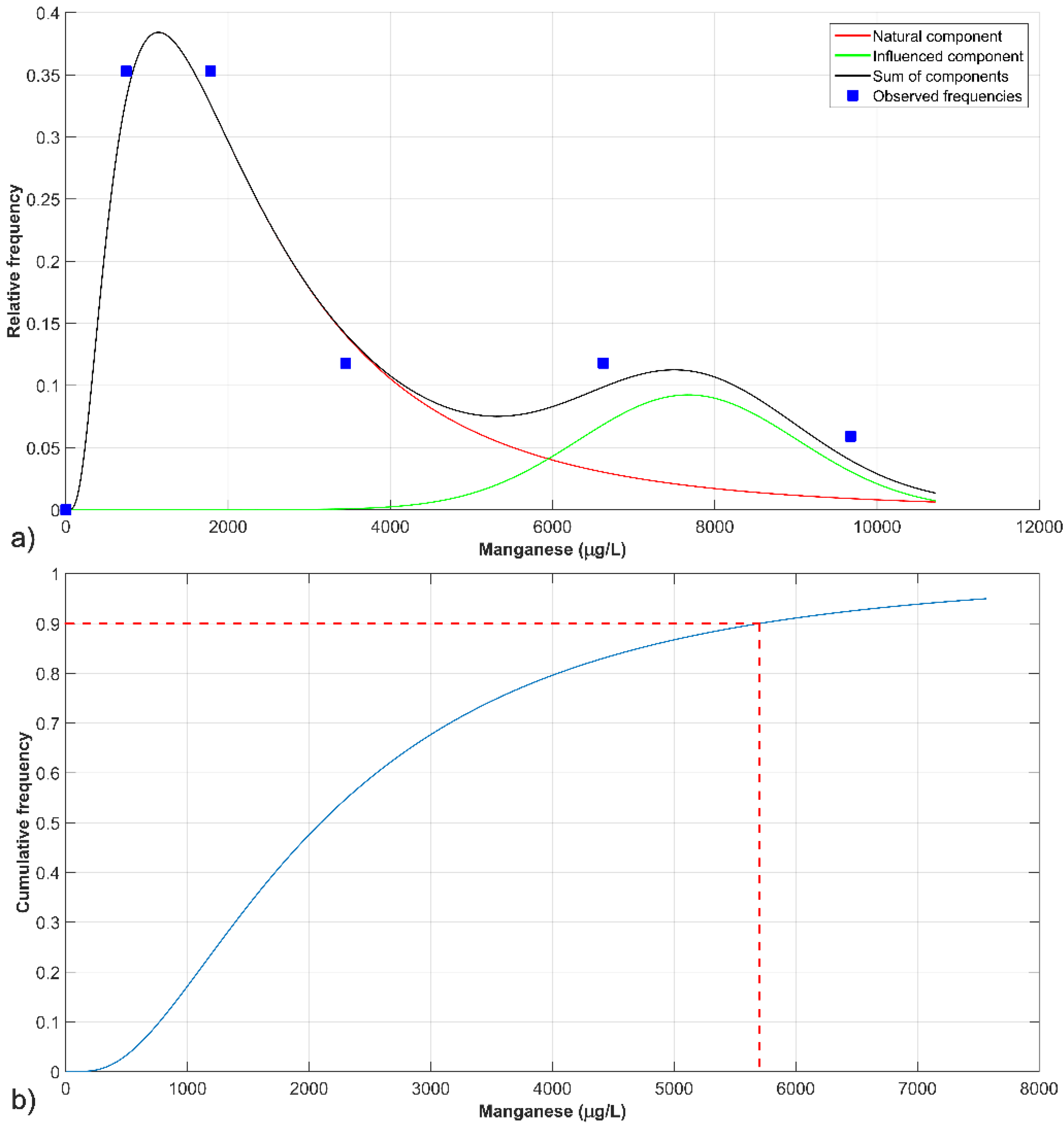
3.1.3. Manganese
4. Discussion
- The input data must come from a single aquifer or a portion of it. The study area must have homogeneous characteristics in terms of geological and hydro-geo-chemical properties, since the procedure provides the estimation of a single NBL value assigned to the whole investigated area.
- The investigation scale depends on the spatial extension within which the aquifer homogeneous characteristics are maintained. This means that, depending on the case, the software can be used for local or regional studies. In practical applications, what provides the actual size of the area to be charged with the estimate result is the number and the distribution of the available observation points falling within the zone of homogeneity. The minimum number of observation points, their distribution, and sampling frequencies are discussed in Section 2.1.3 (Blocks CS5-CS7 (NBL reliability)).
- The operator using the software is an integral part of it. He or she makes important decisions by systematizing the information coming from the study of the conceptual model and from the results gradually emerging from the guided procedure. This implies that not everyone is able to obtain reliable results.
5. Conclusions
Author Contributions
Funding
Acknowledgments
Conflicts of Interest
References
- Hinsby, K.; Condesso de Melo, M.T. Application and evaluation of a proposed methodology for derivation of groundwater threshold values-a case study summary report. Report to the EU Project ‘BRIDGE’. 2006. Deliverable D22. Available online: http://nfp-at.eionet.europa.eu/Public/irc/eionet-circle/bridge/library?l=/deliverables/d22_final_reppdf/_EN_1.0_&a=d (accessed on 29 September 2020).
- Edmunds, W.M.; Shand, P.; Hart, P.; Ward, R.S. The natural (baseline) quality of groundwater: A UK pilot study. Sci. Total Environ. 2003, 310, 25–35. [Google Scholar] [CrossRef]
- European Commission. Guidance on Groundwater Status and Trend Assessment, Guidance Document #18; Technical Report; European Communities: Luxembourg, 2009; ISBN 978-92-79-11374-1. [Google Scholar]
- Panno, S.V.; Kelly, W.R.; Martinsek, A.T.; Hackley, K.C. Estimating background and threshold nitrate concentrations using probability graphs. GroundWater 2006, 44, 697–709. [Google Scholar] [CrossRef] [PubMed]
- Walter, T. Determining natural background values with probability plots. In Proceedings of the EU Groundwater Policy Developments Conference, (UNESCO), Paris, France, 13–15 November 2008. [Google Scholar]
- Wendland, F.; Hannappel, S.; Kunkel, R.; Schenk, R.; Voigt, H.J.; Wolter, R. A procedure to define natural groundwater conditions of groundwater bodies in Germany. Water Sci. Technol. 2005, 51, 249–257. [Google Scholar] [CrossRef] [PubMed]
- BRIDGE. Background cRiteria for the IDentification of Groundwater Thresholds. 2007. Available online: http://nfp-at.eionet.europa.eu/irc/eionet-circle/bridge/info/data/en/index.htm (accessed on 27 August 2020).
- Edmunds, W.M.; Shand, P. Natural Groundwater Chemistry; Blackwell Publishing Ltd.: Oxford, UK, 2008; p. 469. [Google Scholar]
- Hinsby, K.; Condesso de Melo, M.T.; Dahl, M. European case studies supporting the derivation of natural background levels and groundwater threshold values for the protection of dependent ecosystems and human health. Sci. Total Environ. 2008, 401, 1–20. [Google Scholar] [CrossRef]
- Wendland, F.; Berthold, G.; Blum, A.; Elsass, P.; Fritsche, J.G.; Kunkel, R.; Wolter, R. Derivation of natural background levels and threshold values for groundwater in the Upper Rhine Valley (France, Switzerland and Germany). Desalination 2008, 226, 160–168. [Google Scholar] [CrossRef]
- Kim, K.H.; Yun, S.T.; Kim, H.K.; Kim, J.W. Determination of natural backgrounds and thresholds of nitrate in South Korean groundwater using model-based statistical approaches. J. Geochem. Explor. 2015, 148, 196–205. [Google Scholar] [CrossRef]
- Preziosi, E.; Giuliano, G.; Vivona, R. Natural background levels and threshold values derivation for naturally As, V and F rich groundwater bodies: A methodological case study in Central Italy. Environ. Earth Sci. 2010, 61, 885–897. [Google Scholar] [CrossRef]
- Stan, C.O.; Buliga, I. Natural background levels and threshold values for phreatic waters from the Quaternary deposits of the Bahlui River basin. Aui Geol. 2013, 59, 51–60. [Google Scholar]
- Sun, L.; Gui, H.; Peng, W.; Lin, M. Heavy Metals in Deep Seated Groundwater in Northern Anhui Province, China: Quality and Background. Nat. Environ. Pollut. Technol. 2013, 12, 533–536. [Google Scholar]
- Molinari, A.; Chidichimo, F.; Straface, S.; Guadagnini, A. Assessment of natural background levels in potentially contaminated coastal aquifers. Sci. Total Environ. 2014, 476–477, 38–48. [Google Scholar] [CrossRef]
- Preziosi, E.; Parrone, D.; Del Bon, A.; Ghergo, S. Natural background level assessment in groundwaters: Probability plot versus pre-selection method. J. Geochem. Explor. 2014, 143, 43–53. [Google Scholar] [CrossRef]
- Chidichimo, F.; De Biase, M.; Straface, S. Groundwater pollution assessment in landfill areas: Is it only about the leachate? Waste Manag. 2020, 102, 655–666. [Google Scholar] [CrossRef]
- ISPRA—Istituto Superiore per la Protezione e la Ricerca Ambientale. Linee Guida per la Determinazione dei Valori di Fondo per i Suoli e per le Acque Sotterranee; Manuali e Linee Guida 174/2018; ISPRA: Rome, Italy, 2018; ISBN 978-88-448-0880-8.
- Tiedeken, E.J.; Tahar, A.; McHugh, B.; Rowan, N.J. Monitoring, sources, receptors, and control measures for three European Union watch list substances of emerging concern in receiving waters—A 20 year systematic review. Sci. Total Environ. 2017, 574, 1140–1163. [Google Scholar] [CrossRef]
- Xiao, F. Emerging poly- and perfluoroalkyl substances in the aquatic environment: A review of current literature. Water Res. 2017, 124, 482–495. [Google Scholar] [CrossRef]
- Tursi, A.; Chatzisymeon, E.; Chidichimo, F.; Beneduci, A.; Chidichimo, G. Removal of Endocrine Disrupting Chemicals from Water: Adsorption of Bisphenol-A by Biobased Hydrophobic Functionalized Cellulose. Int. J. Environ. Res. Public Health 2018, 15, 2419. [Google Scholar] [CrossRef]
- Tursi, A.; De Vietro, N.; Beneduci, A.; Milella, A.; Chidichimo, F.; Fracassi, F.; Chidichimo, G. Low pressure plasma functionalized cellulose fiber for the remediation of petroleum hydrocarbons polluted water. J. Hazard. Mater. 2019, 373, 773–782. [Google Scholar] [CrossRef]
- De Vietro, N.; Tursi, A.; Beneduci, A.; Chidichimo, F.; Milella, A.; Fracassi, F.; Chatzisymeon, E.; Chidichimo, G. Photocatalytic inactivation of Escherichia coli bacteria in water using low pressure plasma deposited TiO2 cellulose fabric. Photoch. Photobio. Sci. 2019. [Google Scholar] [CrossRef]
- Barnett, V.; Lewis, T. Outliers in Statistical Data, 3rd ed.; Wiley: Chichester, UK, 1994; 584p. [Google Scholar]
- Huber, P.J. Robust Statistics; John Wiley and Sons: Hoboken, NY, USA, 1981. [Google Scholar]
- Walsh, J.E. Large sample nonparametric rejection of outlying observations. Ann. I. Stat. Math. 1958, 10, 223–232. [Google Scholar] [CrossRef]
- Dixon, W.J. Processing Data for Outliers. Biometrics 1953, 9, 74–89. [Google Scholar] [CrossRef]
- Rosner, B. On the Detection of many outliers. Technometrics 1975, 17, 221–227. [Google Scholar] [CrossRef]
- Mann, H.B. Nonparametric tests against trend. Econometrica 1945, 13, 245–259. [Google Scholar] [CrossRef]
- Kendall, M.G. Rank Correlation Methods; Griffin: London, UK, 1975. [Google Scholar]
- Shapiro, S.S.; Wilk, M.B. An analysis of variance test for normality (complete samples). Biometrika 1965, 52, 591–611. [Google Scholar] [CrossRef]
- D’Agostino, R.B.; Stephens, M.A. Goodness-of-Fit Techniques; Marcel Dekker Inc.: New York, NY, USA, 1986. [Google Scholar]
- Lilliefors, H.W. On the Kolmogorov-Smirnov Test for Normality with Mean and Variance Unknown. J. Am. Stat. Assoc. 1967, 62, 399–404. [Google Scholar] [CrossRef]
- Box, G.E.P.; Cox, D.R. An analysis of transformations. J. R. Stat. Soc. B 1964, 26, 211–252. [Google Scholar] [CrossRef]
- ISO 16269-6, Statistical Interpretation of Data, Part 6: Determination of Statistical Tolerance Intervals, Technical Committee ISO/TC 69, Applications of Statistical Methods. Available online: https://www.iso.org/obp/ui/#iso:std:iso:16269:-6:ed-2:v1:en (accessed on 27 August 2020).
- Puls, R.W.; Barcelona, M.J. Ground Water Issue: Low-Flow (Minimal Drawdown) Groundwater Sampling Procedures; Technical Report EPA/540/S-95/504; US EPA: Washington, DC, USA, 1996. [Google Scholar]
- D.Lgs. 152/06—Decreto Legislativo n. 152 del 3 aprile 2006. Norme in materia ambientale. Pubblicato nella Gazzetta Ufficiale n. 88 del 14 Aprile 2006—Supplemento Ordinario n. 96. Available online: https://www.gazzettaufficiale.it/dettaglio/codici/materiaAmbientale (accessed on 29 September 2020).
- Mc Arthur, J.M.; Ravenscroft, P.; Safiulla, S.; Thirlwall, M.F. Arsenic in groundwater: Testing pollution mechanisms for sedimentary acquirers in Bangladesh. Water Resour. Res. 2001, 37, 109–117. [Google Scholar] [CrossRef]
- Mc Arthur, J.M.; Banerjee, D.M.; Hudson Edwards, K.A.; Mishra, R.; Purohit, R.; Ravenscroft, P.; Cronin, A.; Howarth, R.J.; Chatterjee, A.; Talukder, T.; et al. Natural organic matter in sedimentary basins and its relation to arsenic in anoxic ground water: The example of West Bengal and its worldwide implications. Appl. Geochem. 2004, 19, 1255–1293. [Google Scholar] [CrossRef]
- Peters, S.C.; Burkert, L. The occurrence and geochemistry of arsenic in groundwaters of the Newark basin of Pennsylvania. Appl. Geochem. 2008, 23, 85–98. [Google Scholar] [CrossRef]
- Saunders, J.A.; Lee, M.K.; Shamsudduha, M.; Dhakal, P.; Uddin, A.; Chowdury, M.T.; Ahmed, K.M. Geochemistry and mineralogy of arsenic in (natural) anaerobic groundwaters. Appl. Geochem. 2008, 23, 3205–3214. [Google Scholar] [CrossRef]
- Hung Hsu, C.; Tang Han, S.; Hsuan Kao, Y.; Wuing Liu, C. Redox characteristics and zonation of arsenic affected multy layer aquifers in the Choushui River alluvional fan, Taiwan. J. Hydrol. 2010, 391, 351–366. [Google Scholar]
- Lawati, W.M.; Rizoulis, A.; Eiche, E.; Boothman, C.; Polya, D.A.; Lloyd, J.R.; Berg, M.; Vasquez-Aguilar, P.; Van Dongen, B.E. Characterization of organic matter and microbial communities in contrasting arsenic rich Holocene and arsenic-poor Pleistocene aquifers, Red River Delta, Vietnam. Appl. Geochem. 2012, 27, 315–325. [Google Scholar] [CrossRef]
- Rotiroti, M.; Sacchi, L.; Fumagalli, L.; Bonomi, T. Origin of Arsenic in groundwater from multilayer aquifer in Cremona (Northern Italy). Environ. Sci. Technol. 2014, 14, 5395–5403. [Google Scholar] [CrossRef]
- Carraro, A.; Fabbri, P.; Giaretta, A.; Peruzzo, L.; Tateo, F.; Tellini, F. Effect of redox conditions on the control of arsenic mobility in shallow alluvional acquifers on the Venezia Plain (Italy). Sci. Total Environ. 2015, 532, 581–594. [Google Scholar] [CrossRef]


| Parameter | Natural Component (fnat) | Influenced Component (finf) |
|---|---|---|
| Mean μ (μg/L) | 32.28 | 197.86 |
| Standard deviation σ (μg/L) | 1.02 | 16.96 |
| Mixture weight A | 0.49 | |
| NBL90 (μg/L) | 119.24 | |
| Parameter | Natural Component (fnat) | Influenced Component (finf) |
|---|---|---|
| Mean μ (μg/L) | 13,183.62 | - |
| Standard deviation σ (μg/L) | 0.59 | - |
| Mixture weight A | 1.0 | |
| NBL90 (μg/L) | 27,960.52 | |
| Parameter | Natural Component (fnat) | Influenced Component (finf) |
|---|---|---|
| Mean μ (μg/L) | 2097.65 | 7671.01 |
| Standard deviation σ (μg/L) | 0.78 | 1350.7 |
| Mixture weight A | 0.65 | |
| NBL90 (μg/L) | 5718.20 | |
© 2020 by the authors. Licensee MDPI, Basel, Switzerland. This article is an open access article distributed under the terms and conditions of the Creative Commons Attribution (CC BY) license (http://creativecommons.org/licenses/by/4.0/).
Share and Cite
Chidichimo, F.; Biase, M.D.; Costabile, A.; Cuiuli, E.; Reillo, O.; Migliorino, C.; Treccosti, I.; Straface, S. GuEstNBL: The Software for the Guided Estimation of the Natural Background Levels of the Aquifers. Water 2020, 12, 2728. https://doi.org/10.3390/w12102728
Chidichimo F, Biase MD, Costabile A, Cuiuli E, Reillo O, Migliorino C, Treccosti I, Straface S. GuEstNBL: The Software for the Guided Estimation of the Natural Background Levels of the Aquifers. Water. 2020; 12(10):2728. https://doi.org/10.3390/w12102728
Chicago/Turabian StyleChidichimo, Francesco, Michele De Biase, Alessandra Costabile, Enzo Cuiuli, Orsola Reillo, Clemente Migliorino, Ilario Treccosti, and Salvatore Straface. 2020. "GuEstNBL: The Software for the Guided Estimation of the Natural Background Levels of the Aquifers" Water 12, no. 10: 2728. https://doi.org/10.3390/w12102728
APA StyleChidichimo, F., Biase, M. D., Costabile, A., Cuiuli, E., Reillo, O., Migliorino, C., Treccosti, I., & Straface, S. (2020). GuEstNBL: The Software for the Guided Estimation of the Natural Background Levels of the Aquifers. Water, 12(10), 2728. https://doi.org/10.3390/w12102728