1. Introduction
Optimal Sensor Placement (OSP) algorithms have been developed for various purposes and different types of sensors, often making use of hydraulic models, to find ideal measurement positions in a water distribution system (WDS). Examples are the placement of pressure sensors for pipe roughness calibration [
1] and quality sensors for water quality monitoring [
2].
In the field of water loss detection and leak localisation, OSP algorithms are used to find the ideal number and the optimal positions of flow or pressure sensors. Many OSP algorithms use the sensitivity matrix as described by Pudar and Ligget in 1992 [
3]; for instance, Farley et al. who were the first to develop a methodology to place pressure sensors for leak localization in 2008. They evaluated simulated leaks in a water distribution system and instantaneous Chi Squared Values of pressure changes. The Chi Squared Values are then separated into detected and undetected leaks using a threshold which leads to a binarized sensitivity matrix [
4,
5]. In 2013, this approach was extended by introducing a punishment of sensor positions with a response close to the threshold to find positions with a more clear response [
6].
In 2012, Sarrate et al. used structural analysis of WDS for solving the OSP problem. They introduced a leak isolability index and used Depth-First-Search. However, this algorithm only works for medium sized network [
7]. Therefore Sarrate et al. extended their algorithm by applying graph clustering to reduce the problem complexity [
8,
9]. In 2014, Sarrate et al. combined their methodology with the leak sensitivity matrix [
10].
Pérez et al. also made use of a binarized sensitivity matrix to choose sensor positions that lead to as many unique leak signatures as possible in 2009 [
11]. However, binarizing the sensitivity matrix leads to a loss in information [
12].
In 2013, Casillas et al. subsequently used a non-binarized sensitivity matrix to calculate projections between the sensitivity matrix and a residual matrix, which includes a substitute for real-world measurement data, introducing an error index to minimize the number of incorrectly localized leaks. This error index then also served as objective function [
13]. Casillas et al. proposed another algorithm in 2015, where overlapping leak signatures in the leak signature space are to be minimized [
14].
Pérez et al. developed an OSP algorithm in 2014 to obtain the optimal sensor positions when adding new sensors to an already existing sensor network by evaluating the leak localization results. For this purpose, the maximum distance to pre-calculated leak scenarios and a gravity center of nodes with a correlation of more than 99% of the maximum correlation is minimized [
15].
Cugueró-Escofet et al. developed another sensitivity-based algorithm in 2015 using a relaxed isolation index. Where Casillas et al. aimed to correctly localize as many leaks as possible, Cugueró-Escofet et al. tried to create clusters of geographically close nodes with similar leak signatures [
16].
Steffelbauer et al. extended the algorithm by Casillas et al. in 2016 by introducing a punishment for nodes with a high pressure uncertainty due to uncertain demands. The resulting algorithm (Sensor Placement under Demand Uncertainties—SPuDU) uses an error index analogous to the one defined by Casillas et al. as objective function [
17].
In 2018, Soldevilla et al. proposed an OSP algorithm using hybrid feature selection that tries to maximize the isolability of leaks when using classifier-based leak localization methods [
18].
In 2019, Righetti et al. used a sensitivity analysis of pressure data generated using hydraulic simulations and a correlation analysis to select nodes as sensor positions that are, on the one hand, sensitive to leaks in the system and, on the other hand, uncorrelated with each other to ensure as little redundant information as possible is gathered by the sensors [
19].
The term
Serious Game was first introduced by Clark C. Abt in 1970 in his book
Serious Games. He differentiated between serious and casual games. In his terminology, a serious game is a game that primarily serves educational and training purposes and not entertainment [
20].
To this day, there is no universally accepted definition of the term serious game [
21]. A more modern definition is the following:
A serious game is a digital game created with the intention to entertain and to achieve at least one additional goal (e.g., learning or health). [
21]
Following this definition, a serious game has to be a digital game; the additional goals, however, do not have to be in an educational context. Therefore, other areas are covered by this definition as well. Furthermore, the developer’s intentions are sufficient to apply the term Serious Game, the goals do not have to be met.
Serious Games have already been developed for different fields, i.e., education [
22], healthcare [
23] and climate change [
24] but also for flood and river basin management [
25,
26,
27] and draughts [
28].
Several serious games have been developed in the field of water distribution, as well. Three of them will be described in the following.
The first presented Serious Game is
Aqualibrium [
29], which is the digital version of the real-life competition of the same name. During the competition, 0.28 m long pipes of two different diameters (3 and 6 mm) have to be placed in a grid connecting three empty containers at predefined positions with an inflow point (a container filled with water placed on a stand). The goal is to fill the empty containers equally with one liter of water coming from the inflow point. At least 16 pipes have to be placed at the 24 possible pipe locations, while not creating any dead end pipes. At the end of the competition, the water in the three containers is measured using measuring cylinders or weight scales. The difference in water volume is transformed into penalty points, leading to a ranking of the competitors [
30]. The digital version follows the same rules; however, the system evaluation is based on hydraulic simulation and is run by pressing the corresponding button in the web interface. Already evaluated solutions can be saved and then again loaded afterwards.
SeGWADE (Serious Game for Water Distribution System Analysis, Design, and Evaluation) [
29] deals with the New York tunnel problem. Several nodes in an existing water distribution system do not reach a certain minimum service pressure; therefore, parallel pipes have to be added using diameters between 36 in (0.9 m) and 204 in (5.2 m). The network topology and the resulting different pipe lengths in combination with the chosen diameters lead to different costs that players should keep minimal, while still achieving the predefined minimum pressure at all nodes in the system [
31,
32,
33]. SeGWADE’s user interface presents itself similar to Aqualibrium’s interface, also offering the possibility to save at any point and go back to a saved system variant.
Network Pipe Sizing is in some aspects similar to SeGWADE. In this game, players have the goal of redimensioning different water distribution systems using a set of different pipe diameters, while also trying to reduce the costs and ensuring that a certain minimum pressure is met throughout the system. Five different networks (i.e., levels in the game) can be successively played with an increase in network size and complexity from level to level [
34].
In this paper, we present a novel approach to the OSP problem, mostly abstaining from any elaborate optimization algorithm but by making use of human intrinsic motivation for the optimization process. Therefore, we introduce a new Serious Game called Serious Sensor Placement (SSP) [
35]. SSP is meant to be an example of the implementation of an optimization problem in WDS as a Serious Game that can be used for teaching students about optimization problems, algorithms, and especially the optimal sensor placement problem. Furthermore, it can be used for demonstrating optimization tasks in WDS to a wider audience. Since SSP is conceptualized as a Serious Game, it is also supposed to provide any player with an enjoyable gaming experience, independent from their level of knowledge concerning WDS.
This paper is structured as follows. In
Section 2, we introduce the principles of SSP and describe an already conducted case study before the case study results are compared to optimization results obtained with the optimization algorithm Differential Evolution (DE) in
Section 3. Finally, conclusions are drawn in
Section 4.
2. Methods and Materials
In this section, a methodology to calculate a net coverage of a given set of sensors regarding leak localization is presented first, followed by a description of the new Serious Game Serious Sensor Placement and the conducted case study.
2.1. Net Coverage Calculation
To measure the performance of a set of sensor positions a net coverage in percent of pipes, on which leaks could be localized correctly, was introduced. This net coverage is calculated based on the OSP algorithm by Casillas et al. from 2013. This algorithm was chosen because it allows an explicit distinction between localizable and non-localizable leaks. SPuDU would have allowed for this, as well, but only at the cost of higher complexity following the introduction of punishment of nodes with high pressure uncertainties. Since the methodology of SSP uses the Casillas algorithm, this algorithm is described in the following.
The OSP algorithm by Casillas et al. is based on a leak localization method, where pressure measurements are compared to pre-calculated simulation results using projections. For the computation of these simulation results, leaks are simulated at all possible leak locations one at a time (i.e., leak scenarios). The leak scenario that leads to the best match with the measurement data is then assumed to be the location of the real leak.
To find optimal sensor positions, the OSP algorithm itself uses a sensitivity matrix S representing the sensitivity of nodes to leaks in the WDS and a residual matrix R that contains simulated pressure data as a substitute for real world pressure measurements.
The sensitivity matrix as presented by Pudar and Liggett [
3] comes in the form:
where
m is the number of possible leak scenarios, and
n the number of possible sensor positions. The leak scenarios are calculated using hydraulic simulations where leaks are one at a time simulated at all possible leak locations. Therefore, at position
i a leak of size
f is simulated, and the resulting pressure at position
j,
, is compared to the corresponding pressure in the original, undisturbed model,
. This pressure difference is then normalized according to the leak size resulting in
Furthermore, a mean node sensitivity for position
j,
, can be calculated using the following equation:
The residual matrix is calculated in a similar way. The values in this matrix, however, are not normalized and, for higher robustness, a different leak size can be used. The components of this matrix are, therefore, calculated as
Next, a binary vector
q of length
n is constructed, where
if no sensor is placed at position
i, and
if otherwise:
Using this vector, a diagonal matrix
is built:
To calculate the correlation between the residual and sensitivity matrix for a given set of sensor positions the normalized projections of the residual matrix onto the sensitivity matrix are calculated, resulting in a projection matrix
with its individual components
calculated as
where
is called the transposed residual vector
(i.e., leak scenario
i of the residual matrix) and
the sensitivity vector
j (i.e., leak scenario
j of the sensitivity matrix). The values in this matrix represent the correlation between the “measured” data and the simulated data. If a leak is correctly localized by the algorithm the correlation of residual vector
i and sensitivity vector
j must be the highest if
. Therefore, the values situated at the principle diagonal should be the highest value of each row in the projection matrix.
To evaluate a set of sensor positions, an error index vector
is used, where
if the leak scenario
i can be correctly localized at position
i, and
if otherwise:
Finally, a mean error index
, which also serves as objective function, is calculated:
, therefore, states the ratio of not correctly localized leaks and should be minimized using a suitable optimization algorithm.
A net coverage
is introduced that represents the percentage of correctly localized leaks in the system:
In EPANET [
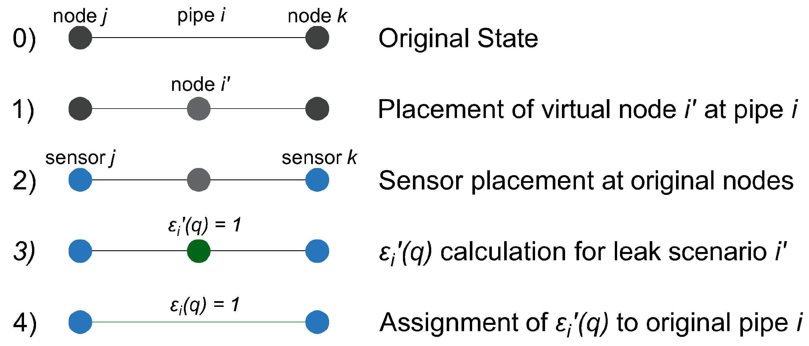
36], leaks are simulated at nodes by increasing the nodal demand or by using a pressure dependent emitter exponent. In SSP, the net coverage is expected to describe the number of pipes in the system, where leaks can be localized correctly. Therefore, to estimate whether a leak at a certain pipe can be localized, the following method is applied:
Placing new nodes (called virtual nodes) in the middle of each pipe.
Situating the sensors at the original nodes in the network.
Calculating the corresponding error index vector of the virtual node .
Assigning the error index of the virtual node, , to the original pipe.
Using this methodology, it is possible to calculate the net coverage achieved by a given set of sensors with regard to leaks at pipes by assigning the individual
to each pipe.
Figure 1 shows an example of this procedure.
2.2. Serious Sensor Placement
In this section, the underlying software of SSP is described, as well as the implemented hydraulic models and the graphical user interface (GUI) itself.
2.2.1. Software Backbone
All pre-calculated simulation results were computed using OOPNET, an object-oriented programming interface between EPANET and Python [
37]. OOPNET was used for sensitivity and residual matrix calculation, as well as calculating the achieved net coverage in SSP.
SSP’s backbone itself is Flask [
38], a WSGI (Web Server Gateway Interface) web framework written in Python that allows for the easy development of WSGI applications. The network is visualized using Leaflet [
39], an open-source JavaScript library that was developed for displaying interactive 2D maps. Finally, PostgreSQL [
40] was chosen as the results database. All solutions submitted by the players are stored in this database, with their usernames hashed for anonymity.
Since the computationally most demanding task, the calculation of the residual and sensitivity matrices, is done beforehand and the net coverages are calculated on a central server, SSP can be accessed and played even on devices with low processing power, like tablet computers.
2.2.2. Hydraulic Models in SSP
Two different hydraulic models have been implemented in SSP so far:
the hydraulic model used by Poulakis et al. for demonstrating leak detection using a Bayesian probabilistic framework [
41] and
C-Town, which was developed for the Battle of Water Calibration Networks [
42].
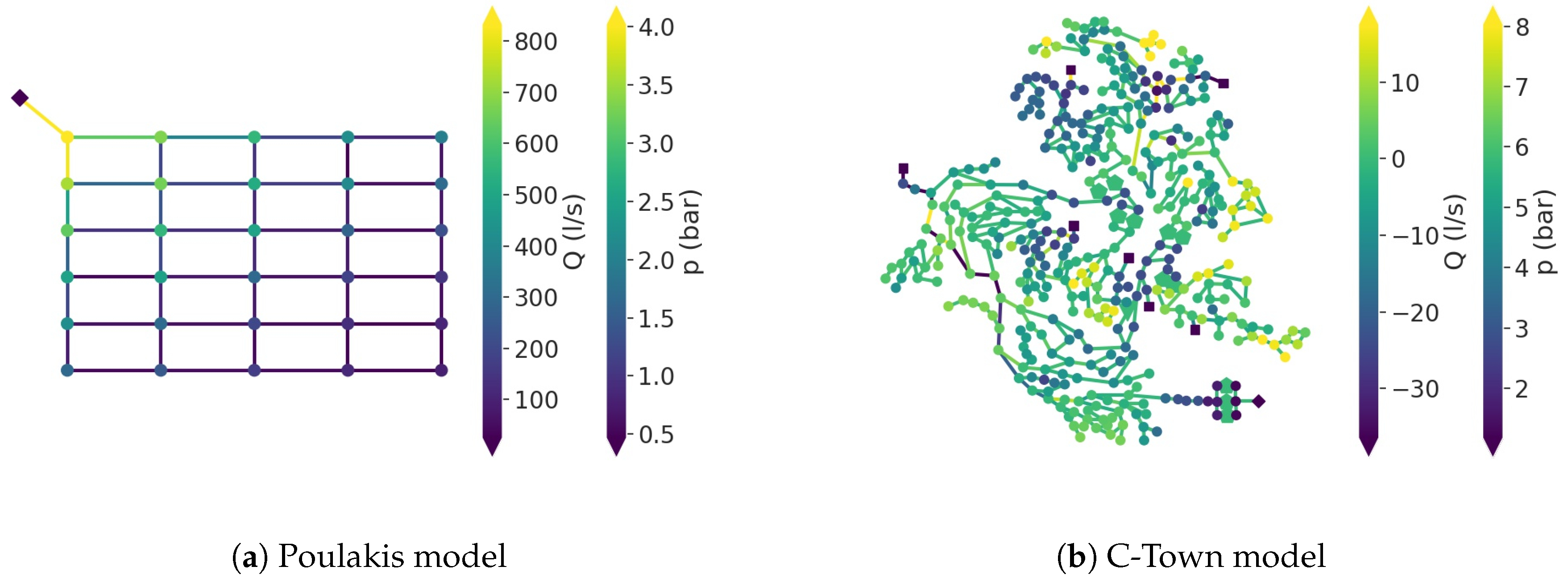
Figure 2 shows the two used hydraulic models and the occurring flows and pressures.
The Poulakis model consists of 50 pipes, 30 junctions, and one reservoir (the diamond shaped symbol in the top left corner of
Figure 2a). The junctions are arranged in a
grid and connected by 1000 m long horizontal and 2000 m long vertical pipes. Diameters range from 300 to 600 mm, and the total length results in approximately 73 km.
C-Town is more complex than the Poulakis model, consisting of one reservoir, seven tanks (represented by squares in
Figure 2b), five pumps, and one throttle control valve and one check valve, as well as 388 junctions and 432 pipes with a total length of approximately 57 km and diameters ranging from 51 to 610 mm.
The two chosen models serve different purposes: Since the Poulakis model consists of only a few links and nodes, the optimization of sensor positions is relatively simple. This allows putting the focus on the game mechanics, hence the use for demonstrating SSP or as a tutorial for first time players.
C-Town, however, is a much more complex network and was chosen to create a more demanding gaming environment.
Sensitivity and residual matrices were calculated, as shown in
Section 2.1, using a fixed leak size of 2 L/s for the Poulakis model and 50 L/s for the C-Town model. No other leak sizes were tested since the optimal sensor positions in a network are not dependent on the leak size used for sensitivity and residual matrix computation [
43]. The results were then exported as geoJSON files together with model component IDs, coordinates, types and status (open or closed).
For easier handling when visualizing the network using Leaflet, the sensitivity values were normalized to values from 0 (low sensitivity) to 1 (high sensitivity).
As using only normalized sensitivities for visualization purposes resulted in very few nodes showing high sensitivities, the sensitivities were finally not only normalized but also logarithmized. This was done to not overstate the absolute node sensitivities’ importance, since the node sensitivity itself is not directly linked to the goodness of a sensor position.
Figure 3 shows a histogram depicting the difference between the two different normalization methods.
The normalized and logarithmized sensitivity of node
j is calculated using the following equation:
where
is the minimum sensitivity, and
is the maximum sensitivity of all nodes.
2.2.3. Game Objectives
The players of SSP are supposed to pursue two objectives while playing SSP:
To set these goals, OSP calculations were made, using the Casillas algorithm and Differential Evolution [
44] for optimization. To get a first overview of the achieveable net coverages, the number of placed sensors was varied from two to 30. All OSP calculations were made optimizing 100 individuals over 100 generations.
Based on the optimization results, the game objectives were then defined for the C-Town model as follows:
Figure 4 shows the calculated net coverages, as well as the part of the solution space that fulfills both objectives. On the one hand, these goals are meant to be achievable since the minimum net coverage can be reached by placing only ten sensors but challenging, on the other hand, because the net coverages achieved by DE are only slightly above this goal. Furthermore, a higher net coverage can only be realized by placing much more sensors. A net coverage of 80%, for instance, can only be reached by using at least 29 sensors. This would pose a significantly more complex task for the players without much additional benefit.
2.2.4. Graphical User Interface
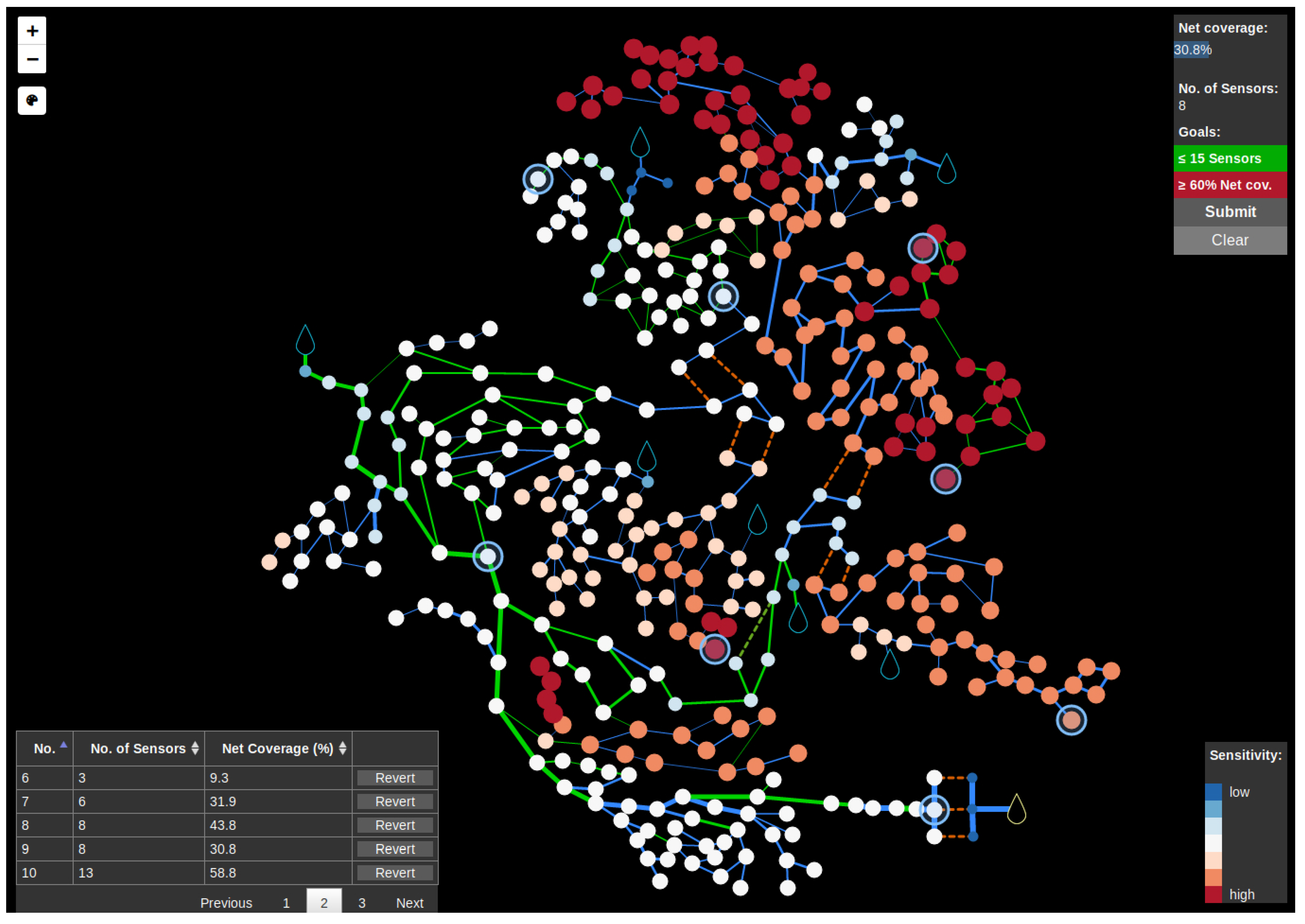
Figure 5 shows the SSP GUI when playing the C-Town model after having placed eight sensors.
The largest part of the GUI is reserved for the visualization of the hydraulic model. The model itself is visualized analogous to the EPANET models using nodes for junctions, tanks, and reservoirs and edges for pipes, valves, and pumps. Sensors can be placed at all nodes except reservoirs, which deliver water with a constant pressure and, therefore, cannot be used for leak localization based on pressure sensors. Tanks and reservoirs are depicted as water drops in either blue (tanks) or yellow (reservoirs). Line widths are either based on pipe diameters or set to a constant value for other link types (e.g., pumps).
A box in the top right corner shows the number of placed sensors, the achieved net coverage resulting from the last submitted solution, and the objectives defined for the players. The button Submit starts the net coverage calculation and then updates the achieved net coverage and the number of placed sensors. Furthermore, the submitted sensor placement and its evaluation results are saved in a PostgreSQL database. A real time evaluation is not achievable due to computation times of about 2 s per set of sensor positions. The minimal net coverage and maximum number of sensors are displayed in front of a red background as long as they are not met. When a player meets one objective, the corresponding background changes to green. The Clear button removes all placed sensors and resets the number of placed sensors and the achieved net coverage.
The table in the bottom left corner allows one to revisit previously submitted solutions. The table shows a consecutive index, the achieved net coverage, and the number of sensors used. Players can sort the table by all three columns in either ascending or descending order. A fourth column contains a Revert button per row that players can use to reload the solution in the corresponding line.
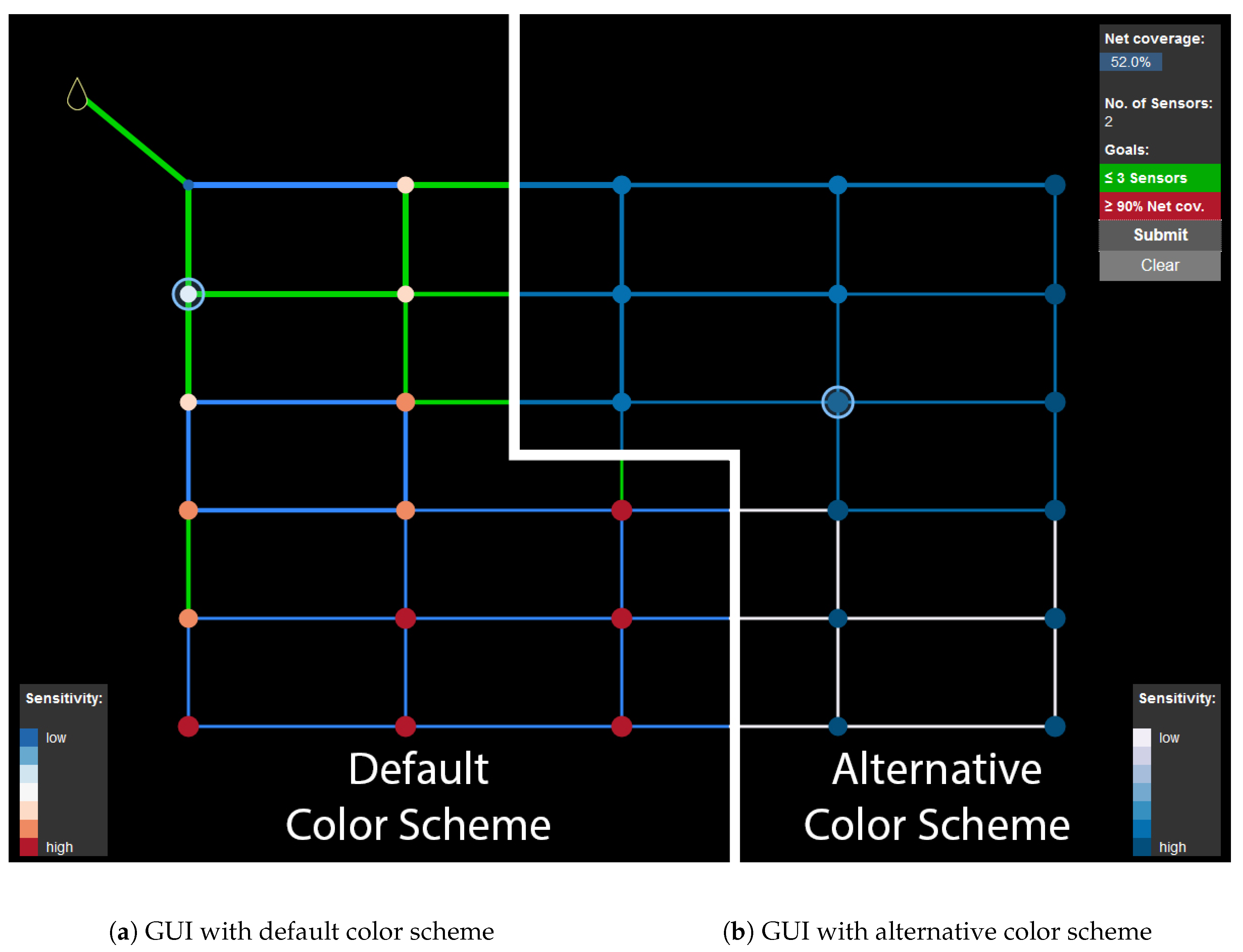
In the top left corner of the screen, two buttons for zooming in and out and a button for switching between two color schemes (a Leaflet EasyButton [
45] showing a Font Awesome icon [
46]) are arranged. The default color scheme shows pipes in either green or blue, depending whether leaks on this pipe can be correctly localized or not. The alternative color scheme uses dark blue and white for this purpose. Node color and diameter depend on the pre-calculated nodal sensitivities as described in Equation (
11). The default color scheme uses a color gradient ranging from dark blue (low sensitivity) to white (medium sensitivity) to dark red (high sensitivity). Alternatively, a color gradient from light grey (low sensitivity) to dark blue (high sensitivity) is used. This alternative color scheme is solely based on color contrast and is especially tailored to persons with impaired color vision. Furthermore, nodes with a low sensitivity present themselves with smaller diameter than nodes with a high sensitivity. The node diameter of node
j,
, is calculated as follows:
where
and
are predefined maximum and minimum node diameters, and
is the normalized logarithmized sensitivity of node
j.
Figure 6 shows the two different color schemes using the Poulakis model after having placed and evaluated two sensors.
2.3. Case Study
SSP was tested in a case study by 12 players. The testing group consisted of ten students, all working in the field of urban water management, with six focusing on water distribution systems. Furthermore, one programmer and one professor, who also specialized on water distribution system analysis, took part in this case study. The level of knowledge concerning WDS research, the optimal sensor placement problem, and mathematical optimization in general, therefore, varied in the testing group.
During the case study, the participants were first informed about the principal idea behind OSP. SSP itself was then introduced using the Poulakis model. It was demonstrated how to place and evaluate sensor positions. Further, the different control elements of SSP, like the buttons for changing the color scheme, were explained. Afterwards, the testers had 20 min to find ideal sensor positions in the C-Town model. Finally, the test persons were asked to anonymously evaluate SSP using a questionnaire.
Four different criteria were evaluated in the manner of school grades from 1 to 5 (lower is better):
4. Conclusions
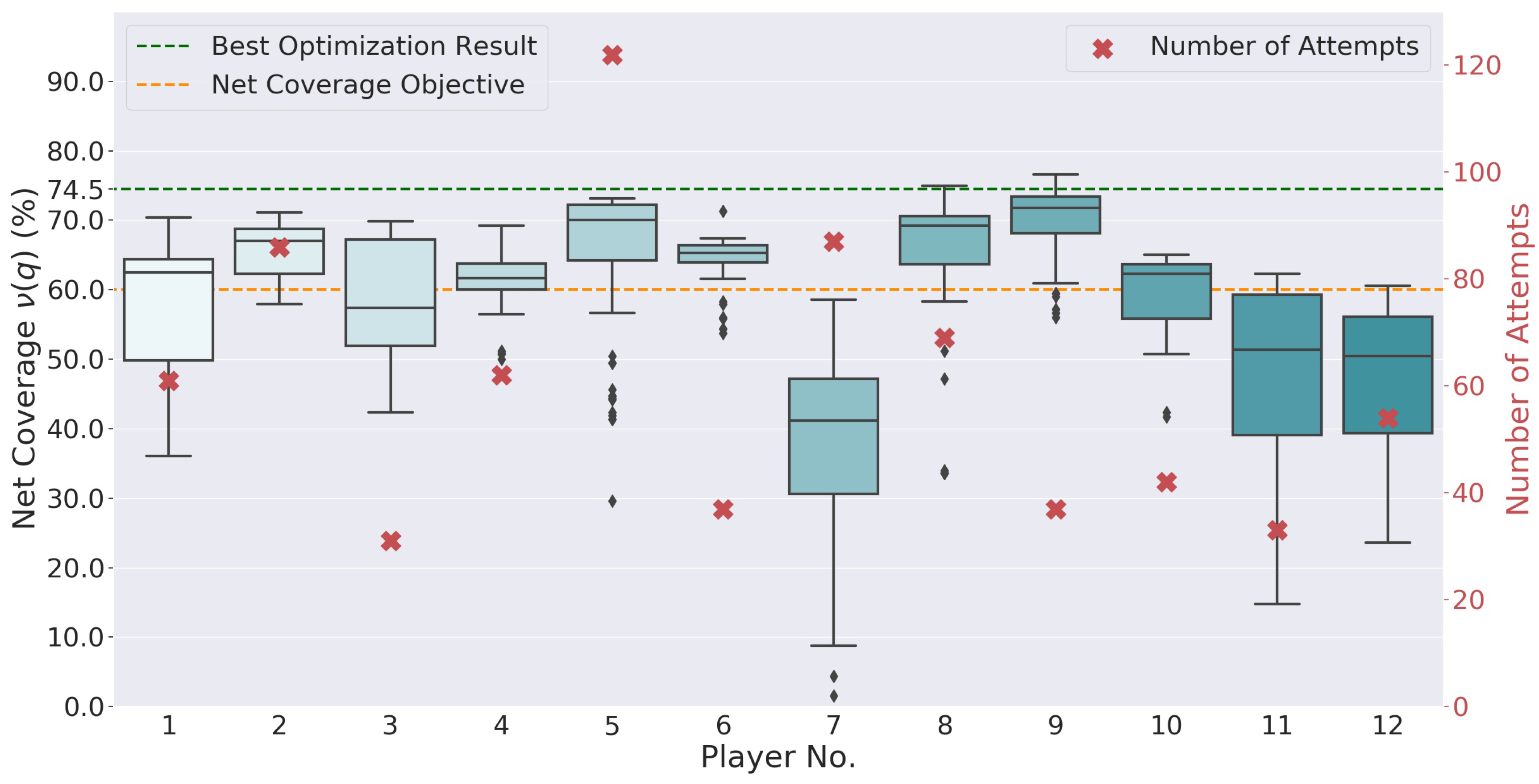
In this paper, a novel Serious Game in the field of water distribution research was presented. For this game, a net coverage with regard to leak localization capabilities based on the optimal sensor placement algorithm by Casillas et al. was introduced. On the one hand, a minimum net coverage should be reached by the players, while on the other hand, a maximum number of placed sensors should not be exceeded.
The game itself was implemented combining Flask, Leaflet, and PostgreSQL based on calculations made using OOPNET. Afterwards, the Serious Game was tested by 12 players who tried to find ideal sensor positions in the C-Town model. During the 20-min-long case study, the testers were able to reach results similar to those obtained through DE, while also enjoying the game experience. Since the testers in the case study were mainly students, SSP was tested in a setting that represents its main purpose: education. The questionnaire evaluation showed that the overall rating was positive and that the game intention (i.e., to motivate the players to further improve their solutions) was met. However, some players recommended improvements of the GUI. Still it can be said that even the current simple GUI was sufficient to activate a player’s intrinsic motivation to optimize his/her results.
Although SSP was only used for educational purposes so far, it could be helpful to demonstrate optimization tasks in WDS to a wider audience, as well.
In general, solving optimization problems with gaming approaches instead of classical optimization algorithms has the advantage of the users being able to apply their knowledge and expertise to solve the problem. The usage of "serious" planning tools, for instance, might lead to more practical results and could increase the commitment of the users compared to optimization-based approaches.
The presented Serious Game itself could also be extended to be used as a planning tool, since Leaflet is originally meant to be used for interactive 2D maps and could, therefore, be adapted to display real world WDS. However, further components would have to be implemented in SSP to create a suitable planning tool (e.g., cost estimations or the possibility to designate nodes, where the installation of measurement devices is infeasible).
Another aspect that should be investigated further is the impact of the level of a player’s knowledge on the quality of his/her results. Due to the anonymized results obtained during our case study and the small number of testers, we were yet unable to quantify this influence.


