Use of Energy-Based Domain Knowledge as Feedback to Evolutionary Algorithms for the Optimization of Water Distribution Networks

Abstract

The optimization of water distribution networks (WDN) has evolved, requiring approaches that seek to reduce capital costs and maximize the reliability of the system simultaneously. Hence, several evolutionary algorithms, such as the non-dominated sorting-based multi-objective evolutionary algorithm (NSGA-II), have been widely used despite the high computational costs required to achieve an acceptable solution. Alternatively, energy-based methods have been used to reach near-optimal solutions with reduced computational requirements. This paper presents a method to combine the domain knowledge given by energy-based methods with an evolutionary algorithm, in a way that improves the convergence rate and reduces the overall computational requirements to find near-optimal Pareto fronts (PFs). This method is divided into three steps: parameters calibration, preprocessing of the optimal power use surface (OPUS) results, and periodic feedback using OPUS in NSGA II. The method was tested in four benchmark networks with different characteristics, seeking to minimize the costs of the WDN and maximizing its reliability. Then the results were compared with a generic implementation of NSGA-II, and the performance and quality of the solutions were evaluated using two metrics: hypervolume (HV) and modified inverted generational distance (IGD+). The results showed that the feedback procedure increases the efficiency of the algorithm, particularly the first time the algorithm is retrofitted.

1. Introduction

Water is the source and sustenance of life, as it has unique properties that make it essential for all living things. However, there are still many people who do not have access to drinking water due to the investment and maintenance costs of water distribution systems (WDS). This problem is very common in developing countries. For this reason, one of the most common optimization problems is the minimum cost design of WDS, which serves to determine the diameter of the network pipes satisfying hydraulic conditions. Moreover, in recent years the optimal design of WDS has changed because a second objective was included in the optimization problem. For solving the new design problem, it was necessary to change from single-objective formulations to bi-objective formulations to obtain a Pareto front (PF) that includes a set of different optimal solutions.

It has been found that the optimal design in WDS belongs to the category of non-deterministic polynomial time-hard problems (NP-hard problems) [1], because of the polynomial given by the equations for energy conservation and the presence of discrete variables. This implies that finding an optimal solution using deterministic and exhaustive methods becomes practically impossible for real-sized networks. However, approximate methods can be implemented to provide near-optimal solutions. Different approaches have been made, including linear and nonlinear programming approximations [2], but metaheuristic algorithms replaced these approaches due to their easy applicability, a greater analysis of the solution space, and their ability to include the constraints given by the discrete-sized diameters. Some of the most common metaheuristic algorithms are genetic algorithms [3], simulating annealing [4], harmony search [5], shuffled frog leaping algorithm [6], and particle swarm optimization [7].

Another alternative, less explored due to the development of metaheuristic methods, was to compute and analyze the optimal design for simple networks and determine some patterns in the results and the hydraulic principles that generate them, to apply them in more complex systems. One of the first researchers to carry out this type of research was Wu [8], who developed an optimal criterion for the design of drip irrigation systems with uniform demands and varied topography. After analyzing many scenarios, he concluded that the optimal design was obtained by the hydraulic gradient line (HGL) followed a parabolic shape with a sag of 15% with respect to a straight HGL. In 1983, Featherson and El-Jumaily [9] suggested applying Wu’s criterion to looped networks. This procedure assumes an initial set of diameters for the pipes, and then adjusting them to fit an ideal hydraulic gradient line. Subsequently, Takahashi et al. [10] introduced the optimal power use surface (OPUS) methodology for looped networks, based on the optimal HGL criterion and other hydraulic criteria. In 2020, Saldarriaga et al. [11] implemented the OPUS methodology in four different benchmark networks to compare the efficiency of applying hydraulic principles with other metaheuristics algorithms. They concluded that OPUS is a suitable method that can be easily applied to real networks, minimizing construction costs in a lower number of iterations than other methodologies.

Nevertheless, the design of drinking water distribution systems cannot be based exclusively on the least-cost criterion, since other variables are also crucial for determining the optimal design solution, such as network resilience and reliability or water quality. For this reason, in the last two decades, multi-objective evolutionary algorithms (MOEAs) have been used to efficiently explore the solution space finding a suitable approximation of the PF. Deb et al. [12] proposed a non-dominated sorting-based multi-objective evolutionary algorithm (NSGA-II), which has been used on multiple occasions for the optimal design of WDS. For example, Farmani et al. [13] used the NSGA-II to minimize cost and number of nodes with head deficiency in a real benchmark network. Similarly, Prasad and Park [14] used the same methodology for designing a WDS, with the objectives of minimizing costs and maximizing the network resilience, obtaining a set of Pareto optimal solutions for two benchmark networks.

As stated before, reliability has become an important objective to guide the optimal design of water networks besides the cost. Hence, regarding the reliability of a WDS, it can be divided into two categories: mechanical and hydraulic. Mechanical reliability refers to the degree to which the WDS can continue to provide adequate levels of service during an atypical event [15]. One of the most widely used indicators of mechanical reliability for the analysis of WDS is the entropy reliability indicator (ERI) [16]. On the other hand, hydraulic reliability refers to the tolerance of the network for changes over time, such as demand variations [15]. Some of the most used indexes for measuring hydraulic reliability are Todini’s resilience index (RI), network resilience index (NRI), minimum surplus head (MSH), total surplus head (TSH), and modified resilience index (MRI)[16]. To determine which indicator best describes the reliability of the network, multiple authors have made comparisons between different indexes. Raad et al. [17] compared four reliability measures, three commonly used (RI, NRI, and flow entropy) and a new mixed reliability measure, by applying them in three WDS benchmarks. In conclusion, the RI showed the best performance under a demand variation, while NRI and the mixed reliability measure performed better after pipe failure conditions. Creaco et al. [18] compared entropy and two reliability indexes (NRI and RI) in two case studies with different topologies to determine which indicator best describes the reliability of a WDN. As a result, they obtained that the index that best describes the reliability of a simple and complex network is NRI. However, it is important to clarify that these indexes are not a measure of network resilience in some cases. Thus, Zhan et al. [19] compared four resilience-related indexes, that included Todini’s resilience index and three direct performance indicators for the optimization of three WDS networks. The results showed the existence of high correlations between the four resilience-related indicators, which served to improve the system resilience measure using any other index. However, each one of the indicators showed both advantages and disadvantages. For instance, Todini’s resilience index showed a high correlation with the direct resilience indicator in the networks without a water tank, but this index should not be used in networks with tanks because the correlation is weaker for those networks.

Hybrid algorithms have recently been developed to extend search efficiency within the solution space. Raad et al. [20] applied a meta-algorithm called AMALGAM and the jumping-gene genetic algorithm (NSGA-II-JG) to the design of WDS. The objectives of the design were to minimize cost and maximize a resilience measure. By implementing all the methods in one case study, AMALGAM obtained the best-quality results in comparison with NSGA-II and NSGA-II-JG. To determine the efficiency of different MOEAs, Wang et al. [21] compared five different multi-objective evolutionary algorithms in twelve benchmark networks. The MOEAs tested include two modern hybrid MOEAs: Ɛ-MOEA and Ɛ-NSGA-III, and three frequently used MOEAs: NSGA-II, AMALGAM, and Borg MOEA. They concluded that the NSGA-II is one of the best MOEAs, because it showed the best achievements in all the benchmarks. Furthermore, from the implemented MOEAs, Wang et al. [21] determined the best Pareto front for each benchmark network. Most recently, Cunha and Marques [22] developed a new multi-objective algorithm based on simulated annealing, including the new generation and re-annealing procedures (MOSA-GR) to minimize the total cost of pipes and maximize the network resilience for the design of WDS. By using this algorithm, there was an improvement in the convergence and diversity of the solutions found in the PF. Initially, it implements a new process for the generation of individuals. After these solutions are obtained, a new stage begins where the re-annealing procedure is implemented to improve the non-dominated individuals found. As a result, MOSA-GR improved the PF obtained by the MOEAs; it generated new solutions that redefine some parts of the best-known front and extended the established boundaries for nine benchmark networks (New York, Blacksburg, Hanoi, GoYang, Fossolo, Pescara, Modena, Balerma and the Exeter network). However, for the other three study cases (two-reservoir, two-toops and BakRyan networks) classified as small networks, the true PF were established by Wang et al. [21]. Given the size of their search space, a complete enumeration can be performed, reaching the true PF. Hence, no further improvements are possible to reach [22].

On the other hand, new hybrid algorithms have been developed from the combination of two methodologies. The first to propose a low-level hybrid procedure were Creaco and Franchini [23], who combined linear programming and the multiple objective genetic algorithm NSGA-II for the design of a group of branched networks. The new algorithm showed benefits in terms of computational and numerical efficiency. More recently, Yazdi et al. [24] developed a hybrid algorithm called non-dominated sorting harmony search differential evolution (NSHSDE), which is the combination of differential evolution (DE) and harmony search (HS). This new method was compared to NSGA-II, strength Pareto evolutionary algorithm II (SPEA-II), and MOEA/D. They obtained that NSHSDE provided better optimal solutions than the other MOEAs used.

The application of evolutionary algorithms (EA) to the WDS optimization problem may require high computational costs, due to their complexity. As a solution in recent years, engineering knowledge has been implemented to decrease the size of the initial population or the search space to obtain good results of the PF in less computational time. Keedwell and Khu [25] implemented a cellular automata approach for the design of WDS. In the generation of the initial population, they applied three rules which related the head at each node and the diameter of the pipes. For example, if the junction had a head deficit, it was necessary to increment the diameters of the pipes connected to that node.

On the other hand, Kang and Lansey [26] used engineering judgment to improve the results of genetic algorithms when applying it to the design of WDN. To determine the initial population of individuals, they used engineering knowledge about optimal flow velocities in WDNs. Bi et al. [27] developed a high-quality initial population by using the multi-objective prescreened heuristic sampling method (MOPHSM) for the optimal design of WDS. The MOPHSM assigns the diameter of the pipe depending on its distance to the source of water and the optimal flow velocity. More recently, Liu et al. [28] determined the first generation of individuals of GA, using a new methodology called head-loss-based design preconditioner (HDP). This method calculates the initial diameter of the pipes by analyzing head losses from the network. HDP was implemented in three WDS networks and compared with prescreened heuristic sampling method (PHSM) made by Bi et al. [29]. Finally, the results showed a better performance for HDP method in terms of computational cost and quality solution.

In order to evaluate the quality of the PFs generated by using MOEAs, different metrics are used. Among the most used are hypervolume index (HV), generational distance (GD), spacing (S), coverage set (CS), inverted generational distance (IGD+), and diversity comparison indicator (DCI). Bi et al. [27] used three run-time performance metrics to understand the speed at which the proposed multi-objective algorithm generated the PF for the optimization of cost and resilience of a WDS. The metrics used were hypervolume, generational distance, and extent of the front. Similarly, Yazdi et al. [24] analyzed four different metrics to solve the same problem, but they used a hybrid algorithm that combines the global search structure of differential evolution (DE) with the local search skills provided by harmony search (HS). Based on previous studies, the hypervolume (HV) and modified inverted generational distance (IGD+) were used in this research to evaluate the performance of the proposed algorithm, due to their advantages in respect to the properties of the PFs that they take into account, such as uniformity and convergence, among others.

This paper aims to present a methodology for the optimal design of water distribution networks (WDN), minimizing the capital cost of the system and maximizing its reliability. However, the proposed methodology seeks to emphasize the improvement of the convergence rate of the NSGA-II algorithm by using constant feedback from an optimal design reached using an energy-based method, in this case, the optimal power use surface (OPUS) [10]. First, a description of the optimization problem is made in which the objectives to maximize and minimize are described, including the corresponding constraints. Then, a description of OPUS and NSGA-II algorithms is presented as an introduction to the bases for the feedback procedure. Both NSGA-II and the proposed algorithm were tested in four benchmark networks (Hanoi, Fossolo, Modena, and Balerma), reaching an approximation to the optimal PF used as a reference [21]. Afterward, the performance of the algorithms was evaluated using the hypervolume (HV) and the modified inverted generational distance (IGD+). Finally, the results are shown and analyzed, evidencing that in three of the tested cases, the proposed algorithm reached a good-quality solution with increased efficiency, delivering better performance for large realistic networks. Hence, using an energy-based method to feedback an evolutionary algorithm was successfully proven as an efficient way to improve the convergence rate for these widely used methods.

2. Optimization Problem

The optimal design problem in WDSs is addressed as a multi-objective approach that seeks to (1) minimize the constructive costs of the network, and (2) maximize a reliability-based index of the network. In this research, the reliability of the network is assessed using a performance measurement known as the network resilience index (NRI), which is founded in the Todini’s resilience index [30]. However, this index incorporates both the effects of surplus power at the nodes and reliable loops in the system, considering the uniformity in the diameters connected to a node [14]. The two objectives used in this approach can be described as follows:

Minimize Cost:

$$C_{Total}={\displaystyle \sum }_{i=1}^{np}{U}_c·D_i·L_i$$

(1)

Maximize NRI

$$\mathrm{NRI}=\frac{{{\displaystyle \sum }}_{j=1}^m{U}_{j}D{M}_j\left(H_j-H_j^{*}\right)}{{{\displaystyle \sum }}_{r=1}^R{q}_r{H}_r^R-{{\displaystyle \sum }}_{j=1}^{m}D{M}_j\left(H_j^{*}+z_j\right)};U_j=\frac{{{\displaystyle \sum }}_{p\in M}{D}_p}{\left|M_j\right|·\underset{pϵM_j}{\max }\left\{D_p\right\}}$$

(2)

where C_Total is the total network cost, which includes the material and construction costs; np is the total number of pipes; D_i and L_i stand for the diameter and the length of the i-th pipe; and U_c corresponds to the unit pipe cost for the D_i diameter. Regarding the network resilience index, U_j represents an indicator for diameter uniformity; H_j and DM_j are the pressure head and the nodal demands for the j-th node; H_j^* is the minimum allowable pressure head at the j-th node; q_r and H_r^R are the total demands and total heads provided by the supply source, respectively; z_j is the elevation of the j-th node; D_p is the diameter that belongs to a set M_j, which represents all the pipes that are connected to the j-th node, and |M_j| is the cardinality of M_j.

The proposed optimization problem is subject to several constraints. In the first place, for service purposes, a minimum pressure is required in the demand nodes, whereas to avoid operational inconveniences, maximum pressure is required, as well as a maximum velocity in the pipes of the system. Secondly, the hydraulic constraints of the network must be met, which include mass and energy conservation in nodes and pipes, respectively, and finally, the selection of a discrete set of diameters for the pipes. While the hydraulic constraints are met by using a hydraulic simulator, such as EPANET, the service constraints were handled by using cost-to-completion static penalty functions incorporated into the algorithm and activated in case the constraints were not met.

The pressure constraints were handled by penalizing the objective functions according to the pressure penalty shown in Equation (3), which considers both minimum and maximum pressures. In this expression, PS_i stands for the maximum pressure surplus in the network, calculated as the difference between the pressure at each demand node and the maximum allowable pressure correspondingly; PS_max corresponds to the maximum allowable pressure surplus within the network; P_min stands for the minimum pressure required at each junction and NMP is the network minimum pressure registered for each individual.

$$Pressure Penalty=\max \left\{\frac{P{S}_i}{P{S}_{max}},\left(\frac{P_{min}-NMP}{P_{min}}\right)\right\}*P_{Ratio}$$

(3)

Similarly, the velocity constraint was ensured by using the velocity penalty shown in Equation (4). In this expression, V_max corresponds to the maximum velocity allowable in the pipes, and NMV stands for the network’s maximum velocity registered for each individual. This penalty function will be used only for the case studies that established a maximum velocity constraint.

$$Velocity Penalty=\max \left\{0,\left(\frac{V_{max}-NMV}{V_{max}}\right)\right\}*P_{Ratio}$$

(4)

Finally, the parameter P_Ratio used in both penalty functions establishes the magnitude of the penalization for the pressure and velocity penalties. This value ranges between 1E06 and 1E09, depending on the tested network, and it was calibrated with the other parameters of the algorithms, as described later in this paper.

3. Methodology for the Optimal Design of Water Distribution Systems

3.1. OPUS

OPUS is an optimized WDS design methodology based on the HGL criterion introduced by Wu [8] and other hydraulic criteria. In order to understand the energy flow of the network, the OPUS methodology is implemented in six steps. First, OPUS—a spanning tree structure is identified for the looped network based on two basic hydraulic principles: (1) the water demand of each node must be supplied from the water sources using a single route for the least-cost WDS case; and (2) the determination of an equation that relates the pipe diameter and its cost per length unit [11]. The first hydraulic principle is based on the fact that redundancy is hydraulically inefficient, even though it increases reliability. For this reason, this process aims to decompose the looped network into a spanning-tree because looped systems can be more expensive than open networks [10]. From this process, it is possible to identify the nodes that can be considered as sumps (i.e., nodes with a lower head than those that are nearby) [10]. The other principle uses the Hazen–Williams equation to determine that as the design flow rate of a pipe increases, the marginal cost decreases [11]. The spanning-tree begins to be built from the water source and increases by adding adjacent nodes, always ensuring that the search front reaches the highest cost-benefit value. This process ends until all the systems nodes have been added to the spanning tree [11].

The second step, optimal power surface, is to determine the head-losses of each pipe by assigning a target HGL for every node [11]. First, a minimum permissible pressure value is assigned to all sump’s nodes. Then, the HGL is calculated using the topological distance from each node to the reservoir and its head. It is possible to determine a series of parabolic functions that serve to find objective head values for each node using the topological distances and the head of each source and sump [10]. The methodology proposed by Ochoa [31] was used to estimate the optimal sag value. This value depended on the ratio between flow demands and pipe length, the cost function, and the demand distribution. The sag value should be calculated at each intersection; hence, the flow on each downstream route must be weighted [32]. For avoiding the assignation of head values that do not meet the pressure demand, nodes with high elevations should be analyzed. Once this process is finished, the optimal power use surface must be formed since all the nodes are assigned an objective head value [10].

The third step, known as optimal flow distribution, consisted of finding a single flow distribution in the network that describes the optimal power use surface calculated in the previous step, ensuring the mass conservation at each node. The optimal flow distribution is calculated by dividing the flow demand into the upstream pipes, starting from the sumps. Saldarriaga et al. [32] created three criteria for this procedure: (1) uniform distribution, where all pipes have the same flow, therefore the flow demand of each node is divided into the number of upstream pipes connected to it; (2) proportional distribution, where the flow is distributed proportionally to H/L², where L is the length of the pipes and H its head losses; and (3) all-in-one distribution, where all pipes are assigned with the design flow that corresponds to the minimum diameter available. The pipe with the highest value of hydraulic favorability is assigned with the residual flow when design with the minimum diameter is insufficient to transport the total flow demand [11].

Once the head of each node and the flow of every pipe are defined, the method calculates the continuous diameter using the Hazen–Williams or Darcy–Weisbach equations. After calculating the diameters, the method rounds the continuous values to discrete values found on the commercial pipeline list [11]. This approach can be made in multiple ways; however, it was found that the best results are obtained by approximating to the nearest flow. This is done by raising the continuous diameter values to a power of 2.6 and round them [32]. The last process of OPUS ensures all nodes have a pressure higher than the minimum value and reduce the diameters of the pipe, without violating any restrictions, to decrease capital costs.

3.2. NSGA-II

One of the most widely used multi-objective evolutionary algorithms in engineering optimization problems is NSGA-II, developed by Deb [12]. For the design of WDS, it has been used to determine the diameter of the pipes with the objectives of minimizing costs and maximizing a measure of reliability [21]. The procedure of the NSGA-II is as follows: first, the algorithm generates a random population between the upper and lower boundaries specified. Then, the individuals are sorted according to non-domination and crowding distance. The elements of the population are selected by the tournament method to create a mating pool with the best individuals. Those selected parents create new individuals by crossover and mutations. Once these processes have been finished, the population is twice as large as the original, in order to select the best individuals of these new population the process of rank and crowding distance must be done again.

In this research, the algorithm has been used to design WDS minimizing cost and maximizing a reliability surrogate measure, such as the NRI [21] by choosing the decision variables as the diameters of each pipe, allowing them to take values from an available diameters list. Finally, NSGA-II was implemented in this research because it is widely used for the design of WDS; however, any other multi-objective evolutionary algorithm could be used instead.

3.3. NSGA-II with Intermittent Feedback from Energy Based Methods

The proposed method (OPUS-NSGA-II) includes the domain knowledge acquired by using OPUS in the NSGA-II metaheuristic. It is divided into three steps as follows: (1) calibration process of the parameters of the tested algorithms; (2) preprocessing of OPUS results; and (3) an intermittent feedback to NSGA-II. These steps are described as follows.

3.3.1. Calibration Process

The calibration process performed in this research consisted of testing different values of the parameters within the recommended ranges and searching to determine a set of parameters that could better approximate the best-known Pareto front for each network.

An optimal set of parameters could be determined by the implementation of systematic approaches, such as optimization. However, these procedures were not applied, given that the proposed methodology sought to provide an improvement in the efficiency of the NSGA-II algorithm rather than the achievement of better solutions than the reported. Hence, the set of parameters determined in this procedure were sufficient to establish a baseline for the comparison between the proposed algorithm and NSGA-II by itself.

In relation with the NSGA-II algorithm, the following seven parameters were considered: population size, number of generations, the crossover distribution index and the crossover probability derived from using simulated binary crossover (SBX), the mutation distribution index and mutation probability derived from the use of polynomial mutation (PM) and finally the P_Ratio for both the pressure and velocity penalty functions. Then, concerning the proposed methodology, the feedback frequency was calibrated. Additionally, every network was tested with a different combination of parameters.

The population size and the number of generations for the study cases varied between (500, 4000) and (500, 5000), respectively, according to the network size. As stated in previous studies, these parameters have a high impact on the computational effectiveness of the algorithm. Hence, enough individuals may avoid a crowded population, while a better convergence can be ensured by performing a larger number of generations [33].

The crossover distribution index considered values that range between 2 and 5, where using greater values ensures fewer variations from parent chromosomes [34]. On the other hand, the mutation distribution index typically ranges between 20 and 100, where greater values also ensure fewer variations from parent chromosomes [35]. Regarding these operators, the probability of crossover and the probability of mutation remained constant and equal to 0.9 and 0.1, respectively, for all the simulations performed. These values were fixed for all networks, given their minor impact on the behavior of the NSGA-II algorithm, as previous studies have demonstrated [33].

For each parameter, the chosen values were selected after a visual inspection in which the convergence to the optimal PF, the spread and distribution of the resulting PFs were the desirable properties. Even though this was not an exhaustive search over the entire parameter space, it covered different values within the ranges, and it allowed the definition of a robust NSGA II for every tested WDS. Moreover, the set of parameters determined by the procedure described above was used in both NSGA-II and the proposed algorithm.

As an example, the comparison between different tested values for the mutation distribution index for Modena after 500 generations is shown in Figure 1.

Regarding the proposed algorithm, the parameter $m$ describes the frequency in which feedback from OPUS is given to NSGA-II, as described in the next sections. For determining the corresponding value for the parameter m at each case study, values between 1 and 100 were tested. This analysis was performed after the other parameters were calibrated, and it sought to determine the best possible values for the parameter to enhance the performance of NSGA-II by the retrofitting process with OPUS. As a result, the effect of this enhancement could be assessed by comparing both algorithms.

After the described procedure was performed, the recommended feedback frequency m was established to be between 5 and 50 generations.

Finally, based on the previous analyses, the calibration procedure was performed, seeking to determine a robust set of parameters for both algorithms, considering each WDS tested. The results of the tests in each case study are described lately in Section 5.

3.3.2. Preprocessing of OPUS Results

The first step requires running the OPUS algorithm up to the step in which continuous diameters are assigned to each pipe (i.e., $D_i\in ℝ \forall i)$. That diameter configuration is used in a hydraulic simulation and the unit-headloss $\left(S_f\right)$ is computed and stored for each pipe.

Then, an envelope curve for the $S_f$ vs. $D$ relationship is computed by using all the unit headloss and diameters for all pipes in the network, as shown in Equation (5):

$$S_f{}_{max}=f_1\left(D\right)$$

(5)

It was found that the function for the envelope curve was always best adjusted by a power function, although this is not a requirement to apply the proposed method.

Then, a pipe friction function relating the flow rate capacity of a pipe $Q$, with the pipe diameter $D$ and the unit head-losses $S_f$, is used (e.g., Hazen–Williams, or Darcy–Weisbach), as shown in Equation (6).

$$Q=f_2\left(D,S_f\right)$$

(6)

Finally, a function representing the OPUS recommended diameter given a flow rate is computed, as shown in Equation (7):

$$Q=f_2\left(D,f_1\left(D\right)\right)=f_3\left(D\right) \to D=f_3^{-1}\left(Q\right)$$

(7)

Considering that $f_1\left(D\right)$ was typically a power function as is $f_2\left(D,S_f\right)$, it was observed that $f_3^{-1}\left(Q\right)$ also was well fitted by a power function.

3.3.3. Intermittent OPUS Feedback to NSGA-II

NSGA-II is applied in the design of WDSs by using the pipe diameter values as the chromosomes, and each particular configuration of diameters in the network as an individual. For computing the performance/fitness of an individual, the cost and NRI objective functions need to be computed, as well as the pressures in the demand nodes to evaluate the compliance of every design with the minimum pressure constraint (as well as maximum velocity constraint if applicable).

The computation of the cost is straight forward—by applying Equation (1). However, the computation of NRI and the minimum pressure constraint requires a hydraulic simulation of the individual’s diameters’ configuration (using a hydraulic simulation engine, in this case, EPANET [36]). This process allows having access to other hydraulic results for each individual, including the flow rate in each pipe.

These values of flowrates can be used as inputs in Equation (7), allowing to compute the OPUS recommended diameters for the particular flow-rates’ configuration of the individual. This new diameter configuration defines the OPUS-updated-individual.

The feedback process starts by taking one generation of individuals from NSGA-II and computing the OPUS-updated-individuals for the whole generation. The following generation is then computed, not by using the crossover and mutation procedures from NSGA-II, but by combining the original individual with their own OPUS-updated-individual. The combination procedure that produces better results (PFs closer to the best-know PF in fewer generations) was found to be a simple averaging between the two individuals, to generate an offspring individual that is tested for fitness and constraint compliance by running a hydraulic simulation as:

$$\begin{array}{cc}individual\hfill & =\left[\begin{array}{c}{D}_1\\ D_2\\ ⋮\\ D_{np}\end{array}\right] ;\mathrm{OPUS}-\mathrm{updated}-\mathrm{individual}=\left[\begin{array}{c}{f}_3^{-1}\left(Q_1\right)\\ f_3^{-1}\left(Q_2\right)\\ ⋮\\ f_3^{-1}\left(Q_{np}\right)\end{array}\right] ;offspring\hfill \\ & =\left[\begin{array}{c}\left(D_1+f_3^{-1}\left(Q_1\right)\right)/2\\ \left(D_2+f_3^{-1}\left(Q_2\right)\right)/2\\ ⋮\\ \left(D_{np}+f_3^{-1}\left(Q_{np}\right)\right)/2\end{array}\right]\hfill \end{array}$$

where $D_i$ is the diameter assigned to pipe $i$ by the original individual, and $Q_i$ is the computed flow rate at pipe $i$ according to the hydraulic simulation of the original individual.

The feedback procedure is used intermittently between generations after a sensitivity analysis showed that continuous or too frequent feedback is detrimental for the spread of the population, generating discontinuous PFs [37]. Therefore, the frequency at which the feedback procedure is applied is a parameter of the proposed method, and the recommended values are $m\in \left(5, 50\right)$, to balance the trade-off between convergence-rate (improved by low $m$ values) and quality of the PF (improved by high $m$ values).

4. Metrics for the Performance of the Algorithms

For studying the effect that adding periodic OPUS feedback has over the NSGA II algorithm’s progress, it was necessary to use a quantitative measure. Bi et al. [27] used three run-time performance metrics to understand the speed at which their proposed multi-objective algorithm generated the PF for the optimization of cost and resilience of a WDS. For this research, these kinds of metrics were estimated in each of the algorithms’ generations, which allows us to see the evolution of the performance of the PFs along with its development. Due to the wide range of metrics available, it was necessary to select the metrics that best described the quality of the PFs obtained with the proposed methodology. After analyzing various metrics and weighing their advantages and disadvantages, the hypervolume (HV) and the modified inverted generational distance (IGD+) were selected. Both metrics were used, because both are unary metrics with uniformity, convergence, and spread quality properties [38]. For both metrics, the fronts were normalized so as not to give more importance to cost respect to resilience.

In the first place, the hypervolume [39] was selected because it is one of the most used indicators and its mathematical properties allow it to be Pareto compliant. This metric indicates the amount of n-dimensional space that is contained by a solution set (the PF) relative to some reference point. In this problem, the optimization algorithms search the best solutions according to two objectives, so the hypervolume is a 2-D space, an area. For a normalized front, the indicator goes from zero to one, where zero is the worst qualification and one is the best. A hypothetical PF that includes a water distribution network with 100% resilience and zero cost would have a hypervolume of one.

The second metric implemented was the modified inverted generational distance (IGD+) [40]. This is a metric that indicates the average separation between a PF and a reference front, in this case, the benchmark front. This indicator is weakly Pareto compliant because it does not consider the distance of the points that are dominated in the reference front. Consequently, the fronts that are entirely equal or better than the reference front will have an IGD+ of zero.

5. Study Cases

The proposed methodology was tested using four water distribution systems, which are well-known benchmark networks. The aim of selecting these networks consisted of testing systems with different sizes, topologies, and even design constraints. As a result, the networks of Hanoi [41], Fossolo [42], Modena [42], and Balerma [43] were used. The characteristics of these networks are shown in

Table 1. Characteristics of the networks used as study cases.

Network	Size 1	Links	Reservoirs	Search Space	Pressure Constraint	Velocity Constraint
Hanoi [41]	Medium	34	1	2.87 × 106	Pmin 30 m	No
Fossolo [42]	Intermediate	58	1	7.25 × 1077	Pmin 40 m Pmax Variable	Vmax 1 m/s
Modena [42]	Large	317	4	1.32 × 10353	Pmin 20 m Pmax Variable	Vmax 2 m/s
Balerma [43]	Large	454	4	1.00 × 10455	Pmin 20 m	No

¹ The size classification is based on [21].

.

For the sake of comparison, two algorithms were tested in the described networks: A NSGA-II algorithm implemented by the authors, and the same NSGA-II retrofitted by the least-cost design reached by OPUS. The parameters required by the algorithms were calibrated following the procedure described in Section 3.3.1 for each network, leading to the values showed in

Table 2. Parameters used for the implementation of the NSGA-II and retrofitted approach.

Network	Individuals	Generations	Mutation Distribution Index	Crossover Distribution Index	Retrofitted Frequency
Hanoi	500	500	20	3	5
Fossolo	500	500	100	10	20
Modena	2000	4000	20	7	50
Balerma	2000	4500	100	2	10

.

Finally, to calculate the hypervolume (HV) and IGD+ metrics for each tested algorithm, the normalization points shown in

Table 3. Reference points used for the normalization of Pareto fronts (PFs).

Network	Cost		Resilience
	Minimum	Maximum	Minimum	Maximum
Hanoi	$15,885,458.05	$111,518,300.50	19.39%	37.15%
Fossolo	€121,012.49	€11,745,019.15	28.19%	100.00%
Modena	€12,412,466.10	€126,059,584.60	34.27%	100.00%
Balerma	€11,898,698.50	€121,068,892.60	37.38%	100.00%

were used to avoid distortions in the results. These reference points were selected as the most extreme points of each objective, both in the best front obtained in the tested methodologies and the benchmark front [21]. Moreover, there was considered a 5% tolerance on each objective, in addition to the most extreme points.

6. Results and Discussion

As a result of this multi-objective optimization procedure, a PF was obtained for each tested approach, considering both the capital costs of the network and the corresponding network resilience index (NRI). In the first subsection below, the evolution along generations of the PFs for each network is shown, considering three different approaches: NSGA-II, NSGA-II with intermittent feedback from OPUS, and the best-known approximation for the optimal PF [21]. Then, the results for the performance assessment of the algorithms are shown, considering hypervolume (HV) and IGD+. The numerical values of the PFs and the metrics are in the Supplementary Materials.

6.1. Approximations to the Best-Known Pareto Fronts

The evolution of the PFs along the tested generations is shown in the figures below for each case study, using a common color-scale where the best-known PF is shown in black, the results for the NSGA-II is shown in light blue, and the results for the retrofitted NSGA-II by OPUS is shown in dark blue.

For the Hanoi network, the evolution of the PFs is shown in Figure 2a–d, showing the results for 50, 100, 200, and 500 generations. In this first case, the NSGA-II algorithm showed a faster approach to the benchmark front for the first 50 generations. However, when the algorithms reached approximately 100 generations, the difference among the approaches tends to reduce significantly. Additionally, the greater differences between the PFs occur during the first generations, but as soon as it overpasses the 200 generations, they do not change considerably. This statement will be discussed later, aided by the performance metrics.

In this case, it is important to highlight that the results for the Hanoi network could be affected by the number of available commercial diameters. Several authors have stated before that the diameters’ list for this benchmark lacks for a higher diameter than the current one, which is 40 in [11]. Consequently, given that the OPUS design is made considering continuous diameters, it is not possible to find a correspondingly good solution when the NSGA-II algorithm tries to round it to the nearest diameter. Therefore, the effect of the retrofitting process is not an advantage for the proposed algorithm, and instead, it slows down its efficiency.

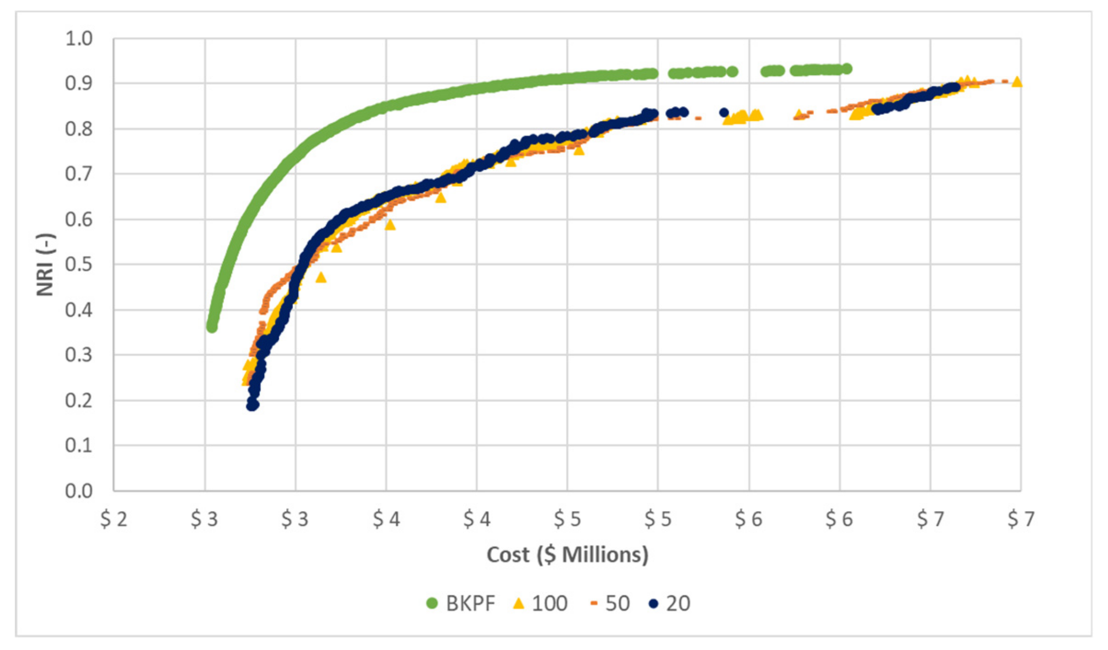
For the Fossolo network, the evolution of the PFs is shown in Figure 2a–d, showing the results for 20, 100, 300, and 500 generations. In this case, the PF obtained using the proposed algorithm is closer to the benchmark front than the obtained by using the NSGA-II by itself since the beginning of the simulations. Additionally, there are some gaps presented in Figure 3a, which are a consequence of the penalty functions used to meet both velocity and pressure constraints. Despite the presence of these gaps, as the algorithm evolves, they tend to disappear until the front is completed. Moreover, the most significant changes in the fronts occurred in the first 200 to 300 generations, and after that, the PF did not change significantly.

The evolution of the PFs for the Modena network is shown in Figure 4a–d, showing the results for 50, 500, 2000, and 4000 generations. Once again, the PF obtained using the proposed algorithm is closer to the benchmark front than the obtained by using the NSGA-II by itself since the beginning of the simulations. Analogous to the Fossolo network, Modena’s design is constrained by a maximum velocity. Therefore, a penalty function was included in the algorithms, explaining the gaps observed in the first 50 generations. In the following graphs, the PF is filled and do not show a significant variation in the last generations.

Finally, the evolution of the PFs for the Balerma network is shown in Figure 5a–d, showing the results for 50, 500, 2500, and 4500 generations. For this network, the proposed algorithm developed with a significant advantage regarding the NSGA-II by itself, as it is shown in Figure 5. Additionally, the approximation of the algorithms described in this research could be closer to the best-known PF if a higher number of generations is used. However, it is important to highlight the increase in the efficiency of the NSGA-II when it is retrofitted by the OPUS algorithm aiming to reach a good solution for the design of the network.

The size of the networks tested seems to have a direct impact on the increase of the efficiency reached by the algorithm when it is retrofitted by an energy-based method such as OPUS. When a medium network such as Hanoi was tested, the difference in the PF between the proposed algorithm and the NSGA-II by itself was not as significant as they were when Balerma, a large water supply system, was tested.

6.2. Results for Performance Metrics

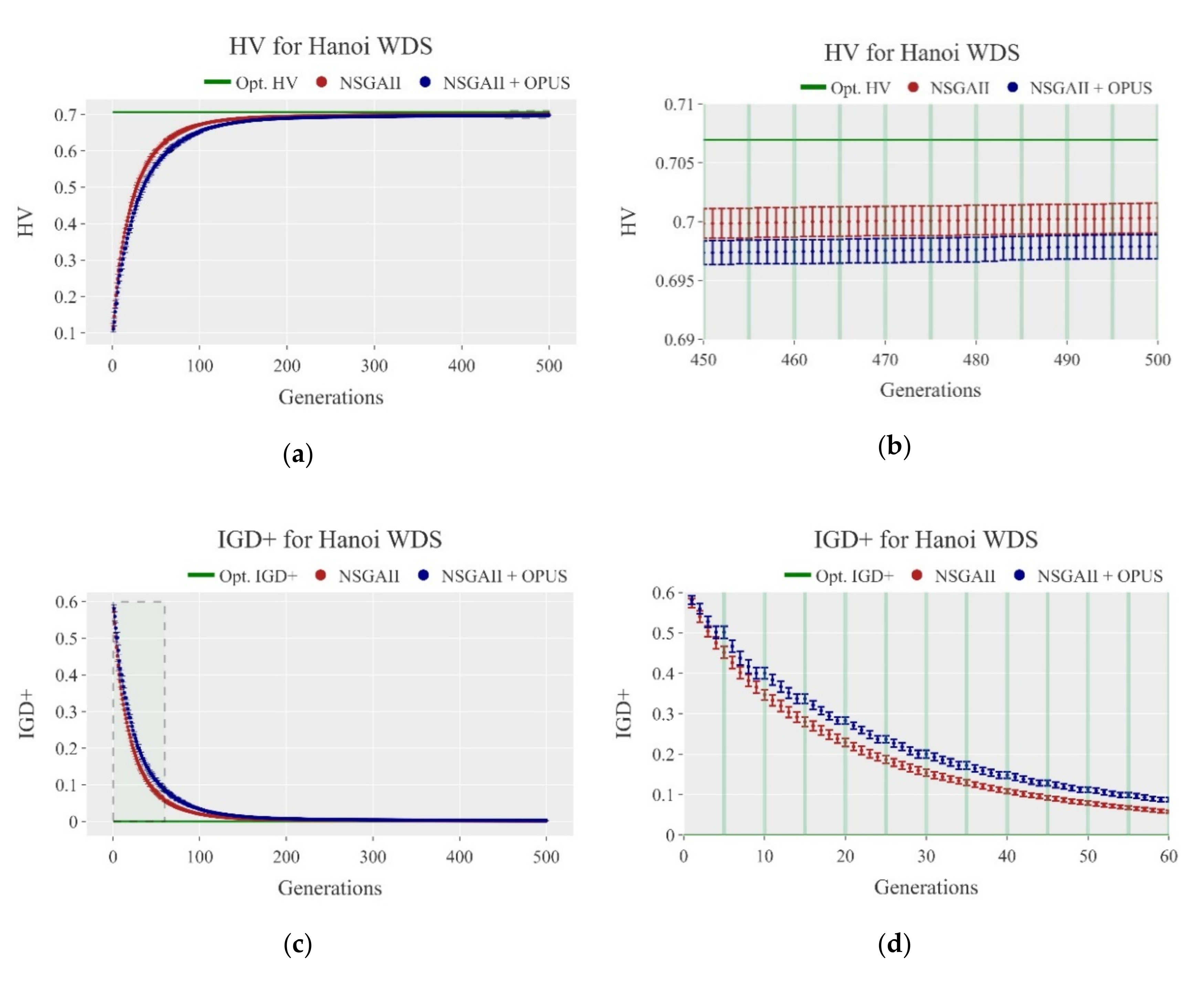
The assessment of the performance of the tested algorithms was performed using hypervolume (HV) and modified inverted generational distance (IGD+). Thus, the evolution of the metrics for NSGA-II and the proposed algorithm are shown in Figure 6a–d, and Figure 7a–d for the HV and IGD+, respectively, organized from the smallest (Hanoi) to the largest (Balerma) tested networks. In the mentioned graphs, the results for NSGA-II are shown in red, the proposed algorithm in green, and the corresponding value to the best-known PF is shown as a continuous red line.

Additionally, when HV is analyzed, the differences between the best-known PF and the obtained results were 1.83%, −0.35%, 7.10%, and 9.79% for Hanoi, Fossolo, Modena, and Balerma, respectively. In this case, the resulting differences are less than 10%, validating the quality of the results.

In the case of the IGD+, given that the best-known PF corresponds to 0, it is expected that high-quality designs are close to this value. Hence, the IGD+ values obtained for the four tested cases were 0.0041, 0.0045, 0.035, and 0.028, respectively, supporting the conclusion led by the HV.

Nevertheless, regarding the performance of the algorithms, the results for both HV and IGD+ metrics show the advantage of the retrofitted algorithm respect to the NSGA-II itself, specifically during the first generations, where the more significant gaps occur as a measurement of the acceleration in the convergence rate of the algorithms. Moreover, the metrics show that for Hanoi and Modena networks, both algorithms tend to converge to a similar value after a certain number of generations. However, in Modena, the jump resulting from the feedback helps the proposed algorithm to stabilize in earlier generations than NSGA-II by itself. Regarding Fossolo and Balerma, a similar result is observed, giving a clear advantage to the proposed algorithm.

The quantification of the advantage of the proposed algorithm respect NSGA-II was performed by determining the percentage difference between both. The latter was calculated in terms of the HV showed in Figure 6, resulting in a positive value the generations in which the retrofitted algorithm obtained a higher HV than the evolutionary algorithm by itself, and a negative value otherwise. Hence, the results for this approach is shown in Figure 8a–d for the four tested networks.

In these plots, Hanoi was retrofitted with a frequency of 5 generations, which is reflected in the oscillatory trend during the first 100 generations. Although the results for Hanoi showed this behavior, the other case studies presented an evident trend in their results. Fossolo, Modena, and Balerma showed a percentage difference of 2.07%, 3.32%, and 14.90% respectively in the generation number 20, 50, and 10 correspondingly. Moreover, the generation in which the maximum gap for the HV occurred matches the time for the first feedback using the OPUS algorithm.

However, the gap between the tested algorithms tends to reduce in further feedbacks, until there is a moment when there is not a significant difference in the HV from both algorithms as the number of generations increases. Summarizing, this means that the proposed methodology has a major impact the first time that feedback occurs, and later this effect will tend to be reduced, making OPUS a good hot-start for evolutionary algorithms.

Additionally, in Figure 8, it is confirmed that the magnitude of the gaps obtained by using the proposed algorithm increases with the size of the network, being 2.07% and 3.32% for Fossolo and Modena networks correspondingly (intermediate to large WDN), and of 14.90% for Balerma network, which is the largest of the tested systems.

Furthermore, although several authors have proposed different approaches to the multi-objective design problem for WDS, the results may vary in terms of efficiency, spread, and even the quality of the solutions. Therefore, it is possible to reach slightly better solutions than the best-known PF obtained by Wang et al. [21], except for those networks where their search space is small enough to have a complete enumeration of the solutions, leading to a true PF [22].

As an exemplification, Bi et al. [27] presented a solution for Fossolo and Hanoi networks where the hypervolume (HV) was greater than 0.95, which corresponded to the best-known PF established by Wang et al. [21]. These solutions were accomplished using the multi-objective prescreened heuristic sampling method (MOPHSM). A similar result was obtained by Yazdi et al. [24], where the non-dominated sorting harmony search differential evolution (NSHSDE) algorithm was implemented, reaching for Fossolo network a PF that was better than the best-known PF in terms of the resilience of the solutions. 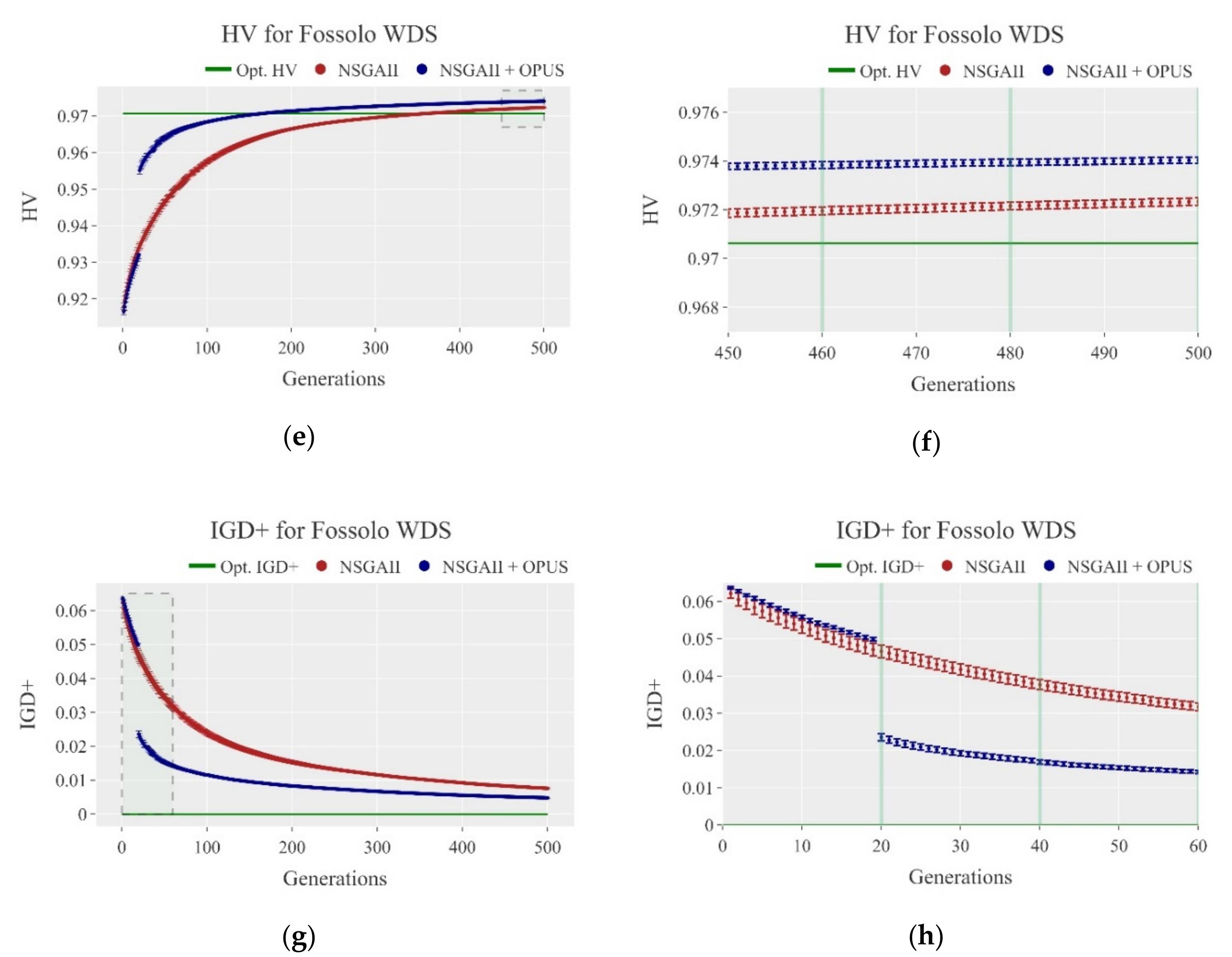In a most recent approach, Cunha and Marques [22] established new best-known PF for nine benchmark networks, classified as medium to large sizes using the multi-objective simulated annealing (MOSA) algorithm, including the Fossolo network. Finally, in this research, authors also reached slightly better solutions for the Fossolo network in terms of its resilience, using the proposed retrofitted NSGA-II algorithm with OPUS as well as the NSGA-II itself. This is validated in Figure 5b, where the HV for both approaches are compared with the best-known results.

6.3. Statistical Analysis of the Results

Due to the inherent randomness of the NSGA II algorithm, it was necessary to perform a statistical analysis of the behavior of the PFs. In such a manner, the effect of using OPUS could be distinguished from mere chance. This evaluation considered the two smaller networks, Hanoi and Fossolo, to assess the performance of the fronts due to their computational speed.

The examination consisted of the execution of 30 simulations of each algorithm for both WDS so that the results drawn from it were statistically valid. Therefore, the values for the metrics as functions of the generations are shown in Figure 9a–h. Each point has a 95% confidence interval calculated using the data from the simulations and a Student’s t distribution with 29 degrees of freedom.

The confidence intervals provide further insights into the development of the PFs. First, the width of the intervals decreased as the algorithm developed. The intervals were wider at the beginning of the process because the solutions were random. Hence, as they were far from optimal, the variance tended to increase. Whereas, at later stages, it was harder to find better solutions as the PFs stabilized. Secondly, the widths of the intervals were small compared to the values of the metrics, which indicated low uncertainty on the results. Although the solutions sampled by NSGA-II were random, the overall behavior of the PFs was stable. Therefore, it produced very similar HV and IGD+ results for different simulations, which, consequently, generated low standard deviations and narrow confidence intervals. Finally, for any generation, after the first OPUS retrofitting occurred, the confidence intervals of both methodologies did not overlap, which indicated that the average values of the metrics were statistically different.

Even though a rigorous statistical analysis requires multiple simulations, the overall behavior of the smaller networks’ PFs (represented by the metrics and their variance) indicates that a single simulation of both algorithms is highly representative of their performance. Therefore, for Modena and Balerma, we implemented this one-simulation approach. These bigger networks involve extensive time and computational cost, and, as previously stated, one simulation is enough to compare sufficiently the algorithms’ functioning.

7. Conclusions

The multi-objective optimal design of WDN, considering the capital costs and the reliability of the systems, was addressed by comparing two approaches: a traditional NSGA-II algorithm and a proposed algorithm in which this evolutionary algorithm was retrofitted with an energy-based method. These methodologies were tested into four well-known design benchmarks (Hanoi, Fossolo, Modena, and Balerma), and then compared their performance and quality of solutions to the corresponding best-known PF [21] using two metrics: hypervolume (HV) and modified inverted generational distance (IGD+). These metrics were selected because they are unary metrics with uniformity, convergence, and spread quality properties [38].

Before the two algorithms were tested in the case studies, a calibration procedure was performed. Although neither an exhaustive nor an optimal search of the values of the parameters were accomplished given the scope of the paper, the set of determined values sought to make a better approximation to the best-known Pareto front within the recommended ranges for each parameter. Hence, after performing several simulations testing different values for each parameter within their corresponding range for each tested network, the values were selected after a visual inspection of the resulting PFs pursuing three characteristics: the spread, distribution, and convergence to the optimal PF. For further research, a wider range of parameters could be tested to analyze their performance in the development of the NSGA-II algorithm.

The set of calibrated parameters were used for both NSGA-II and the retrofitted algorithm to make a plausible comparison between them. Moreover, the retrofitting frequency, or parameter m, was tuned for each network seeking to increase the performance of the proposed algorithm. For further research, it is recommended to test the overall effect of this parameter over the other NSGA-II parameters, as well as its correlation with the size of the networks. Additionally, the calibration procedure could be improved by implementing a systemic approach if the scope of the study is to achieve better PF rather than improving the efficiency of the algorithm.

Regarding Hanoi, the NSGA-II algorithm showed better results than the retrofitted algorithm. This occurs given that the maximum diameter available for this benchmark is not enough to reach a near-optimal design when using energy-based methods, as it has been stated by several authors such as Saldarriaga et al. [11]. Therefore, when OPUS is used to make feedback on NSGA-II, as it performs a continuous design, the input diameters resulting from this process that are greater than 40 in. are going to be rounded off to that value. Hence, the proposed algorithm will lose efficiency because a loop-wide behavior, in which the continuous design from OPUS will try to reach a near-optimal solution with a higher diameter, and NSGA-II will try to round it to 40 in.

Despite the results obtained in Hanoi, in the remaining study cases, the proposed algorithm reached closer solutions to the best-known PF in a more efficient manner than a traditional NSGA-II. Moreover, the feedback process of the proposed algorithm tended to accelerate the convergence of the evolutionary algorithm, which is reflected in the gaps in the HV obtained in the first retrofitting generation for each network: 2.07% in Fossolo, 3.32% in Modena, and 14.90% in Balerma. However, these impacts were substantial only the first time the algorithm was retrofitted, and in further feedbacks, the magnitude of the gaps started to reduce until there is no significant difference between the HV evolution for the tested algorithms.

The previous analysis also made evident an important conclusion: when the PFs were compared, the size of the network seems to play a key role in the efficiency of the proposed algorithm. Hence, when the network is bigger, the impact of the feedback is more significant in the improvement of the solutions. Therefore, the effect of using OPUS for retrofitting the NSGA-II was higher when Balerma was analyzed (14.90% in the first feedback) rather than Fossolo, which was an intermediate-size network (2.07% in the first feedback).

Regarding the HV and IGD+, which were the metrics used for assessing the performance and quality of the algorithms, it can be concluded that they were useful to quantify the closeness of the results obtained against the best-known PF for each network. For HV, the differences between the value obtained for the best-known PF and the results were 1.83%, −0.35%, 7.10%, and 9.79% correspondingly for Hanoi, Fossolo, Modena, and Balerma. In the case of the IGD+, considering that the best-known PF corresponds to 0, then the values obtained for the four tested cases were 0.0041, 0.0045, 0.035, and 0.028 correspondingly. Hence, it can be concluded that the proposed algorithm can reach PFs with a difference of less than 10% regarding the benchmark fronts.

In the results for Fossolo, the HV at the last generation for the proposed algorithm had a difference of −0.35% regarding the best-known PF established by Wang et al. [21], representing a slightly better solution. Similar situations have been exposed by Bi et al. [27], Yazdi et al. [24], and Cunha and Marques [22]. Even though it is possible to improve the quality of the solution slightly in medium, intermediate, and large-size networks, there are small networks in which is possible to perform a complete enumeration given the size of their search space, leading to a true PF and consequently avoiding further improvements [22]. For further research, it is recommended to test a higher number of networks while considering more sizes and topologies than the ones considered in this paper, to explore a potential relationship between the size and characteristics of the networks. Hence, the user of the algorithms will be capable of establishing the potential benefit of using an energy-based method to retrofit an evolutionary algorithm, in this case, NSGA-II, before its implementation.

Additionally, the evolution of the metrics along with the number of generations made evident the behavior of the tested algorithms. During the first generations, the most significant changes in the metrics occurred; as the methodologies developed, the change in the metrics got less significant until they stabilized, meaning that a set of solutions (PF) was reached. This behavior can be oriented to take advantage of two aspects: (1) the use of an approach that allows navigating faster into the search space, as in this case, an energy-based input; and (2) the determination of an optimal number of generations required to reach a near-optimal solution, avoiding additional computational efforts.

The statistical analysis of the PFs’ metrics indicated that the overall behavior of the PFs for different simulations was stable. Consequently, the variances of the metrics for every generation of the algorithms was small, and it decreased as the fronts converged in later generations. Thus, the confidence intervals calculated with these variances were sufficiently narrow to discard multiple simulations. Conversely, it was possible to use a one-simulation approach for every method and still be able to compare them validly. Furthermore, the confidence intervals did not overlap, which indicates that the average values of the metrics were statistically different.

The approach of energy-based methods such as OPUS, to WDS optimal design problem, has the capabilities of reaching near-optimal solutions in a reduced number of iterations; besides, it represents a practical approach for engineers who are not familiarized with optimization procedures. Furthermore, in the algorithm presented in this paper, the capabilities of OPUS are extended to a wider range, allowing it to be a high-quality and feasible start for an evolutionary procedure. Thus, the convergence rate of these algorithms can be speeded up, achieving closer solutions to benchmark PFs, especially in larger networks.

Finally, the proposed algorithm proved that it is feasible to reach a near-optimal set of solutions (or PF) close enough to the benchmark front in an efficient manner. Given that the most considerable effect of the feedback is obtained during the first time the algorithm is retrofitted, derived methodologies should focus on using energy-based methods to perform a hot-start for evolutionary algorithms. Afterward, in further stages of the algorithm, the feedback procedure can be modified to maintain a significant effect on its convergence. However, the proposed methodology presented in this research ensures a good approach to the optimal design problem considering different objectives related to the cost and the reliability of the network.