Abstract
Similarity analysis of small- and medium-sized watersheds mainly depends on manual work, and there is no complete automated analysis method. In order to solve this problem, we propose a similarity analysis method based on clustering ensemble model. First, the iterative clustering ensemble construction algorithm with weighted random sampling (WRS-CCE) is proposed to get great clustering collectives. Then, we combine spectral clustering with the fuzzy C-means method to design a consensus function for small- and medium-sized watershed data sets. Finally, the similarity analysis of small- and medium-sized watersheds is carried out according to the clustering results. Experiments show that the proposed clustering ensemble model can effectively find more potential similar watersheds and can output the similarity of these watersheds.
1. Introduction
Flood disaster is one of the most dangerous natural disasters. In recent years, the management of large rivers has tended to be perfect. However, many small- and medium-sized river basins have not received enough attention in flood control, and hydrological workers cannot issue flood warnings of small- and medium-sized river basins timely. According to incomplete statistics, there are more than 50,000 small- and medium-sized river basins in China, and 85% of the cities are located along the coast of these river basins. The frequent abnormal climate and extreme weather conditions have brought tremendous pressure to flood control in small- and medium-sized river basins these years. Therefore, it is urgent to control flood in small- and medium-sized watersheds. However, many small- and medium-sized watersheds lack corresponding hydrological data, they cannot carry out hydrological analysis, which leads to great difficulties in the management of these watersheds [1]. In hydrology, hydrological analysis is accomplished by parameter transplantation. The first step of parameter transplantation is analyzing the similarity of these unknown watersheds to find similar watersheds [2]. Therefore, it is very important to select appropriate and accurate similar watersheds.
Many hydrological scholars have studied basin similarity analysis. Considering that the differences in spatial distribution of some elements in different watersheds will eventually lead to different hydrological characteristics, Wood and Hebson [3] first proposed the concept of watershed hydrological similarity. Merz et al. [4] first used attribute similarity method to find similar river basins in order to complete parameter transplantation between similar watersheds in 2004. Young et al. [5] chose to use distance nearest algorithm for watershed similarity analysis. In 2006, Young et al. carried out a similarity analysis on 260 UK Watersheds with a distance nearest algorithm. Through the analysis of similar watersheds, the parameters of the missing data watersheds were transplanted. Finally, the accuracy of the similar watersheds was verified according to the transplanted results. Zhang and Chiew [6] consulted the ideas of the former two methods and combined the distance nearest method with the attribute similarity method, which improves the accuracy of watershed similarity analysis. Considering that the concept of watershed similarity is not clearly defined and bounded, we can consider the concept of watershed similarity to be a fuzzy concept. Therefore, Shouyu Chen [7] proposed the use of fuzzy set method to establish a similar watershed selection model and find similar watersheds. Yaya Song proposed a similar watershed optimization algorithm based on fuzzy weighted recognition model [8]. In order to minimize the uncertainty in the optimization of hydrological similar watersheds, Ming Zhang [9] created a maximum entropy optimization model in 2012 by studying the ambiguity and difference in the importance and comprehensive values of the similarity indicators of the data. Li Qisong [10] and Fan Mengge [11] combined Principal Component Analysis (PCA), cluster analysis, and watershed similarity again in 2012 and 2015, respectively. Among them, Fan [11] put forward that the hydrological similar determinants such as multi-year maximum flood peak and flood volume analysis of similar basins should be used to verify the results of similar basin analysis.
Although there have been many related studies, there are still many problems in similarity analysis of small- and medium-sized watersheds. Nowadays, the analysis and determination of similar watersheds basically depends on the artificial decision of hydrological experts. There are many impersonal and inaccurate situations in this way. At present, there is no similar analysis method for small- and medium-sized watersheds, especially clustering ensemble method. Due to the data of small- and medium-sized watersheds often having more characteristic dimensions, the existing watershed similarity analysis methods may not achieve ideal results for such high-dimensional and complex data sets. Therefore, we make full use of the geographical data and hydrological data of small- and medium-sized watersheds and use data mining technology to study and analyze watershed similarity. This paper puts forward a similarity analysis method of small- and medium-sized watershed based on clustering ensemble. The contributions of this paper are as follows:
- (1)
- This paper proposes a novel cluster ensemble model to analyze the similarity problem of small- and medium-sized watersheds.
- (2)
- For small- and medium-sized watershed data, we propose an iterative clustering collective construction algorithm based on weighted random sampling (WRS-CCE) to construct clustering groups with high clustering quality and difference.
- (3)
- For small- and medium-sized watershed clustering groups, we design the corresponding consensus function. We use the connected triple similarity matrix (CTS) as the input matrix of spectral clustering algorithm and combine it with fuzzy C-means (FCM) method to get the final clustering results.
- (4)
- A comprehensive evaluation index (OCQ-NMI) based on quality and diversity is proposed to screen clusters with high quality and diversity in multiple iterations.
2. Basic Theory
In this section, we introduce the hydrological similarity assessment indicators and clustering related theories.
2.1. Hydrological Similarity Assessment Indicators
According to the various hydrological similarity assessment indicators proposed in reference [12] and the existing data situation, we use topographical and meteorological elements, a total of 27 indicators as characteristic indicators of similarity analysis data sets for small- and medium-sized watersheds. The following two categories of indicators are introduced separately.
- (1)
- Topographical indicators. The topographic, geomorphological, and soil conditions of a basin will have a great impact on the generation and change of runoff in the basin. These indicators are the decisive parameters for hydrological simulation and soil erosion prediction [12]. In this paper, 18 topographical and geomorphological indicators are selected as follows: basin area, basin length, basin average slope, morphological factor, elongation ratio, river network density, river maintenance constant, average river chain length, average catchment area of river chain, total length of river network, river frequency, river chain frequency, main channel length of constant flow, ratio gradient of main channel of constant flow, maximum distance of flow path, area of elevation curve of river basin, approximate constant K, and area slope. Eighteen topographical and geomorphological index data need to be extracted from Digital Elevation Model (DEM) data through the toolbox provided by the software and related manual operations. Generally speaking, we need to calculate the runoff direction of DEM area first, identify and fill the marsh, and calculate the runoff direction of non-marsh area. Then the accumulation of confluence is calculated and the grid map of river network can be obtained according to the accumulation of confluence. Finally, the required topographical and geomorphological index data can be extracted from the grid map according to the relevant formulas.
- (2)
- Meteorological indicators. Meteorological elements promote the whole hydrological process of the basin and play an important role in the analysis of hydrological similarity. They make the confluence characteristics of different basins have similarities [12]. In this paper, 9 meteorological indicators are selected as follows: annual average rainfall, average rainfall in flood season (June-September), maximum rainfall in 1-h, maximum rainfall in 3-h, maximum rainfall in 6-h, and maximum rainfall in 12-h. The extraction of 9 meteorological indicators needs to be divided into two main steps. The first step is to get the longitude and latitude information of all stations from the list of stations in the basic hydrological database, then map all stations to the map by ArcGIS software, and find out the coding of one or more stations in each small- and medium-sized watershed. The second step is to extract precipitation data from precipitation excerpt table, monthly precipitation table and annual precipitation table according to these codes, and to process them with Extract-Transform-Load (ETL), finally we can obtain 9 meteorological index data of small- and medium-sized watershed.
2.2. Clustering Algorithm
2.2.1. Clustering Evaluation Index
Here we introduce two index: Clustering Quality (Ocq) and Normalized Mutual Information (NMI).
1. Clustering Quality (Ocq)
Clustering is an unsupervised learning method, so it is necessary to evaluate the quality of the clustering results after the clustering is completed. The quality evaluation of a clustering result is based on the following two indicators: compactness and separation [13]. In reference [14], clustering quality based on clustering density and clustering proximity is proposed as a quality evaluation index for each cluster member.
Clustering Quality (Ocq): By combining clustering density with clustering proximity, an evaluation method can be defined to measure the quality of a clustering result. Its definition is as follows:
where represents clustering intensiveness; represents clustering proximity; is a weight used to represent the ratio between the two, generally set to 0.5, which means that the two are of equal importance.
The clustering quality defined by Equation (1) is for one of the cluster members in the clustering group. Therefore, this paper uses the average of the cluster members’ qualities in the clustering group to represent the entire clustering quality of the entire clustering group, which is defined as OCQ. It can be concluded that the larger the OCQ, the better the clustering quality of the clustering group.
2. Normalized Mutual Information (NMI)
In [15], it is proposed that in integrated machine learning, the greater the inconsistency between the learners of the integrated learning, the better the integration effect and the higher the efficiency. This inconsistency represents the difference between the collectives. If the difference between the groups is greater, it means that the relevance of the learner is lower, which means that the effect of integrated learning is better. Clustering ensemble, as a kind of integrated machine learning, also has this feature. Specifically, the greater the difference between cluster members in the clustering group, the better the clustering integration effect.
Mutual Information (MI) is a measure of the degree of interdependence between two random variables. Unlike correlation coefficients, mutual information is not limited to real-valued random variables. It is generally determined by the joint distribution of two random variables and their respective edge distributions. Its definition is as follows:
where is the joint probability distribution function of and , and are the edge probability distribution functions of and , respectively.
In the literature [16], Strehl and Ghosh normalized the mutual information by using the entropy value of the random variable and proposed the Normalized Mutual Information (NMI). The role of the NMI is to limit mutual information to a range of 0 to 1. First, the definition of the random variable entropy value is given:
Then according to the entropy value of two random variables and mutual information, the standardized mutual information size is obtained. Its definition is as follows:
Applying Equations (2)–(4) to the cluster members, you can get the NMI values between the two cluster members. Its definition is as follows:
where and represent the respective number of clusters of cluster members and ; represents the number of identical data points in the th cluster of cluster member and the th cluster of cluster member ; represents the number of data points in the th cluster of ; represents the number of data points in the th cluster of cluster member .
In order to calculate the difference of the clustering ensemble, the literature [17] proposes to use the average of NMI values between the cluster members in the clustering group as the final NMI value of the entire cluster. The definition is as follows:
where represents the number of cluster members.
2.2.2. Spectral Clustering Algorithm
The spectral clustering algorithm is based on spectral partitioning, which converts clustering into multiple partitioning of undirected graphs [18]. For spectral clustering, clustering of a dataset can be understood as the optimal segmentation of the graphs formed by the dataset. The following are the core steps of spectral clustering:
- (1)
- Add the numbers on each column of the similarity matrix , and after obtaining numbers, fill them into the diagonal position of the matrix (filling zeros at other positions of the matrix), and finally get an . The matrix is recorded as the degree matrix . Then, the Laplacian matrix is obtained from the similarity matrix and the degree matrix .
- (2)
- According to the correlation algorithm, the first eigenvalues and the corresponding eigenvectors of the matrix are obtained in order from small to large.
- (3)
- -character vectors are spliced into a matrix of in a column manner. Each row vector of the matrix is each attribute vector of the -dimensional space. Finally, the algorithm is applied to the matrix to obtain the final Clustering results.
2.2.3. Fuzzy C-Means Clustering
The FCM clustering algorithm is a combination of hard partitioning clustering and fuzzy mathematics theory, which was proposed by Dunn in the literature [19], refined and propagated by Bezdek [20]. In fact, the FCM clustering is a simple change on K-Means, and the membership degree is used to replace the original hard partition, making the edge smoother.
For the input data set , where represents the number of data points, after FCM clustering, a membership degree matrix is obtained, where represents the number of clusters, and denotes the membership degree of the th data point in the data set belonging to the th cluster. The FCM algorithm finds the cluster center that can make the objective function the smallest by continuously iterating and returns the membership matrix at this time.
3. Similarity Analysis of Small and Medium Rivers based on Clustering Ensemble Model
Clustering ensemble applies the integrated learning idea to the clustering algorithm. The main idea is to use a single clustering algorithm to generate multiple cluster members to form a clustering group, and then use the consistency function to cluster the members. This enables the final clustering results to get the information in the cluster members to a maximum extent, which is more accurate than the clustering results of a single clustering algorithm [21].
Cluster integration is mainly divided into two steps. The first step is to construct the cluster collective, and the second step is to design the consistency function. Then, how to construct a high-quality cluster collective based on small- and medium-sized watershed data sets has become the prerequisite for similarity analysis using cluster integration. After we obtain the cluster group, how to design a consistency function for them becomes the key to similarity analysis of that. For the characteristics of small and medium watershed data, this paper first proposes the constructing clustering ensembles by weighted random sampling (WRS-CCE) to obtain high quality clustering groups. Then combining Spectral Clustering (SC) with fuzzy C-means (FCM) clustering algorithm to get clustering results and the specific watershed similarity analysis can be performed. The clustering ensemble processes are shown in the Figure 1.
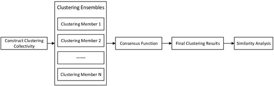
Figure 1.
Clustering Ensemble Processes.
3.1. Constructing Clustering Ensembles by Weighted Random Sampling
Nowadays, most of the studies focus on the design of consistency function, but few on the construction of clustering groups in clustering ensemble. The commonly used traditional clustering collective construction method is to randomly construct clustering members by multiple clustering and the randomness of initialization. This method is difficult to ensure that clustering members have high quality and high diversity. Therefore, we propose an iterative constructing clustering ensembles by weighted random sampling (WRS-CCE) algrithm, and use OCQ-NMI comprehensive index as the evaluation index (shown in Figure 2).
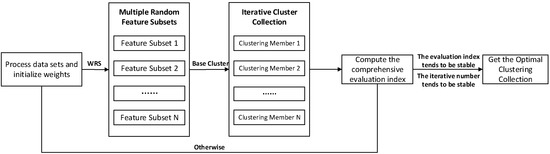
Figure 2.
Iterative constructing clustering ensembles by weighted random sampling.
3.1.1. Constructing Feature Subsets
Since the small- and medium-sized watershed datasets select multiple feature dimensions from the DEM elements and the meteorological elements respectively, it can be said that the datasets have high dimensional data characteristics. So, it is difficult to construct a clustering group with high quality and high diversity at the same time. In this paper, the weighted random sampling method is used to sample the characteristic indicators of data sets to get several different feature subsets. Then, the weights of the characteristic indicators are adjusted in each iteration process. The specific construction steps of the feature subset are as follows:
- (1)
- If it is the first iteration, assign initial weights to all feature metrics of the dataset. Then, according to the weight ratio of the feature index, it is weighted and randomly sampled, and some feature indicators are selected as the feature subset.
- (2)
- The obtained feature subset is input into the iterative algorithm to construct the clustering group. Then we update the weight of the feature index according to the OCQ-NMI index of the clustering group.
- (3)
- Repeat step 1 and step 2 until the number of iterations is met or the iteration is over.
The random sampling ensures that the feature subset can maintain diversity and difference, and the method can reduce the selection probability of the feature index which has bad effects on the cluster by initializing the weight and adjusting the feature index, thereby improving the efficiency of the iteration and stability.
3.1.2. Generating Base Cluster Member
The small- and medium-sized watershed datasets involve a lot of hydrological data and underlying surface data, which are affected by human operations during the acquisition process. Therefore, if the datasets are dimensionally reduced and projected into a two-dimensional space, it will have a lot of noise points. In the traditional clustering group construction algorithm, the algorithm is used for clustering, but the algorithm is easily affected by noise points. Therefore, this paper uses clustering algorithm to replace the commonly used clustering algorithm as the base clustering algorithm, which will effectively improve the quality of clustering members in the cluster group.
First, we need to determine the number of clusters. There is a generally accepted upper limit of the number of clusters, i.e., the maximum number of clusters, which is defined as follows:
Among them, is the maximum clustering number and is the sample number of the data set.
Therefore, this paper will select the commonly used cluster number judgment indicators. After calculating the corresponding cluster number of these indicators, select the maximum value that does not exceed as the optimal cluster number of base cluster. The judgment indicators here include the Dunn index proposed by Dunn [19], the Calinski-Harabasz (CH) index proposed by Calinski [22], and the Davies-Bouldin (DB) index proposed by Davies [23]. Through the comparison of multiple indicators and the limitation of the upper limit of the clusters number, it is possible to obtain the number of clusters that are not too large or too small, and to ensure that the subsequent clustering algorithm can get better clustering results.
The specific steps of cluster member generation are as follows:
- (1)
- Randomly select k data points from the data set and use it as the initial clustering center.
- (2)
- Traverse the points in the data point set, and assign them to the nearest central point according to the distance from the initial cluster center to form k clusters.
- (3)
- Traverse the non-central point p in each cluster, calculate the cost E if we replace the cluster center o with p, and select the smallest p of E to replace the original center point o.
- (4)
- Repeat step (2) and (3) until the cluster center no longer changes.
As a basic clustering algorithm, can perform high-quality clustering on small- and medium-sized watershed datasets which have more noise points, and can get better clustering results and great cluster members to constitute clusters.
3.1.3. OCQ-NMI Comprehensive Evaluation Index
A clustering group is composed of multiple cluster members, and each cluster member in a high-quality clustering group should be different, and the quality of each cluster member is also very important. In this paper, we combine two indicators to get a comprehensive evaluation index and use it as an evaluation index of the WRS-CCE algorithm to select clusters with high quality and high diversity in multiple iterations.
The OCQ-NMI comprehensive evaluation index combines the quality evaluation index based on OCQ and the difference evaluation index based on NMI. It measures the comprehensive quality of clustering group by setting the balance weight of the two. Its definition is as follows:
where represents the balance weight of the cluster member quality and difference, and the greater the , the more affected by the quality of the cluster members. In order to balance the quality and difference of aggregates, the value of is chosen to be 0.5.
It can be seen from the above formula that the larger the OCQ-NMI index is, the higher the quality of the clustering ensemble is, and the greater the difference is. Therefore, the OCQ-NMI indicator can be used as an evaluation index for each iteration in the algorithm.
3.1.4. WRS-CCE Method
In this paper, the WRS-CCE algorithm is used to construct the clustering group of the medium and small watershed datasets, and the OCQ-NMI index is used to evaluate the clusters obtained in each iteration. The algorithm steps are as follows:
- (1)
- Judge the pre-processed data set. Initialize the weight first, and then we use weighted random sampling for feature selection to construct a plurality of different feature subsets.
- (2)
- Use algorithm to perform basic clustering on these feature subsets, and a clustering group containing multiple cluster members is constructed.
- (3)
- Use the OCQ-NMI index to evaluate the clustering collective obtained in this iteration. According to the evaluation result, we need to determine whether to record the clustering ensemble obtained in the current iteration and whether to adjust the weight of the feature index in the specified feature subset. Then restart the next iteration from step (1).
- (4)
- End the iteration after satisfying the number of iterations or the OCQ-NMI comprehensive evaluation index tends to be stable.
After the iteration is completed, we can obtain multiple cluster members based on the small- and medium-sized watershed datasets. These cluster members not only have higher clustering quality, but also have greater differences with each other. They together form clustering ensemble based on small and medium watershed datasets.
3.2. Consistency Function with SC-FCM
The consistency function is a process of clustering and merging all of the cluster members included in the clustering ensemble to obtain the final clustering result. In this paper, for the characteristics of small- and medium-sized watersheds, the Connected Triple Similarity (CTS) matrix is constructed by Weighted Connected-Triple (WCT) algorithm and used as the similarity matrix.
Then, the matrix is clustered and fused by the Spectral Clustering with the fuzzy C-means (SC-FCM). Finally, we can obtain the clustering results and complete the similarity analysis of small- and medium-sized watersheds (shown in Figure 3).
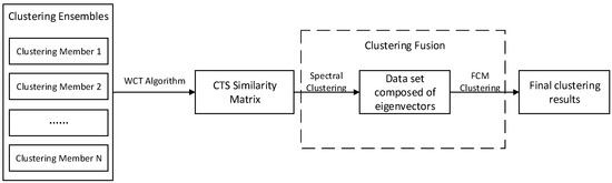
Figure 3.
Spectral Clustering with the fuzzy C-means (SC-FCM) clustering fusion algorithm.
3.2.1. Connected Triple Similarity Matrix
For clustering algorithms, especially the spectral clustering algorithm used in this paper, the clustering effect depends on the similarity matrix. So, the similarity matrix is very important. The traditional similarity matrix generally uses Fred’s similar cross-correlation matrix, mainly because the construction of it is relatively simple. However, its shortcomings are also obvious. First, if the cluster members do not reach a certain scale, the cross-correlation matrix cannot accurately reflect whether the two data points can appear in the same cluster. Second, the matrix can only reflect the similarity between some data points, and the hidden relationship between many data points has not been found. In order to find out the potential similarity between these data points, this paper uses the Connected Triple Similarity Matrix (CTS) proposed by N.Iam-on [24] as the input matrix of the clustering fusion algorithm.
The Connected Triple first proposed by Klinks [+] to solve the problem of repetitive author names when searching for paper authors in the paper database. Its definition is as follows:
For vertex set and edge set , where vertex and vertex respectively have two sides and with the same vertex , then vertex and vertex are considered to be similar. The vertices composed of these three vertices and edges formed by the two sides together form a Connected Triple .
When the concept of Connected Triple is applied to clustering ensemble, it can be understood in conjunction with Figure 4. In Figure 4, denotes the th clustering member, represents the first th data. The superscript of denotes the label of the cluster, and the subscript denotes the label of the cluster members. That is, represents the th cluster of the th cluster member. If belongs to cluster , they are connected by a straight line.
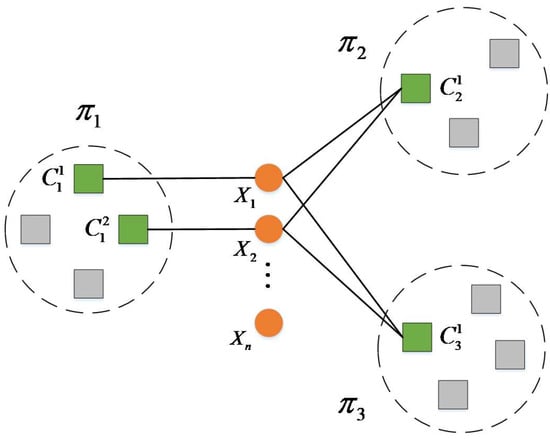
Figure 4.
Application of Connected Triple in clustering ensemble.
According to Figure 4, if we use the concept of cross-correlation matrix, we can only judge that data points and are similar in cluster members and . It is because Cluster in Cluster Member and Cluster in Cluster Member contain both data points and , which belong to Cluster and respectively in Cluster Member . For Interrelation Matrix, data points and are different in Cluster Member . According to the concept of the Connected Triple, since Cluster and Cluster simultaneously contain data point , Cluster and Cluster simultaneously contain data point , Clusters , and Cluster together form a Connected Triple. The Clusters , and also form a Connected Triple. Then, for the Connected Triple, the data points and are similar in the cluster member , and the similarity between the two can be calculated by the WCT algorithm.
The WCT algorithm can calculate and expand the similarity between data points, and finally get the CTS similarity matrix. In WCT, the similarity between data points is calculated by calculating the weight between clusters. Some basic definitions are as follows:
Definition 1.
Data set:, whererepresents the data point and N represents the number of data points contained in the data set.
Definition 2.
Clustering collective:, whererepresents a cluster member and M represents the number of cluster members included in the clustering ensemble.
Definition 3.
Cluster member:, whererepresents the cluster in the cluster member and K represents the number of clusters included in the cluster member.
Definition 4.
Cluster:represents the kth cluster of cluster member.
Equation (9) is given below to calculate the weight between two clusters:
where represents the magnitude of the weight between clusters and , and and represent the set of data points in clusters and , respectively (see Supplementary Material Algorithm S4–S6).
3.2.2. SC-FCM Clustering Fusion Algorithm
The spectral clustering algorithm is based on spectral partitioning, which converts clustering into multiple partitioning of undirected graphs [18]. The spectral clustering algorithm is simple to use, and its processing effect on complex data types is often better than that of direct algorithm.
The FCM clustering is a simple change on K-Means. It uses the membership degree to replace the original hard partition, makes the edge smoother. Compared with the traditional algorithm, FCM clustering algorithm does not impose any specific category on the data object to be clustered. It uses the membership degree (the degree of belonging to this category) to represent the similarity degree of the data objects belonging to each category. This idea corresponds to the purpose of seeking the similarity degree between watersheds in the watersheds similarity analysis. Therefore, we use fuzzy C-means algorithm instead of K-Means method as the final step of spectral clustering algorithm to obtain the final clustering result.
The core step of spectral clustering is to simplify the dimension [25]. We first use the spectral clustering algorithm to deal with the CTS matrix obtained above to get the first k eigenvectors and form an eigenvector matrix. The feature vector in the matrix largely represents the feature information of each data point in the original data set. Therefore, using the CTS matrix as the input can get the eigenvector matrix reflecting the data characteristics of the small and medium watershed dataset. Then, the eigenvector matrix gained from the spectral clustering is used as the data set and input into the FCM clustering algorithm. Finally, we can obtain the clustering result based on the small- and medium-sized watershed dataset and perform the specific watershed similarity analysis.
3.2.3. Consistency Function Based on SC-FCM
This paper constructs the CTS similarity matrix of clustering group based on WCT algorithm, and then uses SC-FCM Clustering Fusion Algorithm to cluster the clustering group, so as to get the final clustering results. The general steps are as follows:
- (1)
- Use WCT algorithm to get the similarity between the data points contained by each cluster and form the CTS matrix.
- (2)
- Transform the CTS matrix into Laplacian Matrix.
- (3)
- Use the Laplacian Eigenmaps (LM) to decompose the matrix, the smallest k eigenvalues and corresponding eigenvectors of the CTS matrix are generated and selected.
- (4)
- The data set consisting of k eigenvectors is processed using the FCM clustering algorithm to get the final result.
According to the clustering results, the final similarity analysis can be performed on the small- and medium-sized watershed.
4. Experiment and Analysis
Small and medium watershed-sized datasets: Generally, the watershed with a drainage area of less than 1 square kilometer is a small and medium watershed, while the water conservancy department in China stipulates that the watershed with a drainage area of less than 50 square kilometers is a small and medium watershed [1].
This paper uses the Digital Elevation Models (DEM) data of Jiangxi as the original data, the resolution is 90 m, with 6708 rows and 5889 columns, totaling nearly 40 million grid cells, and its geographic longitude and latitude range is 24.488927–30.079224 in the north latitude and 113.575079–118.482839 in the East longitude.
Firstly, according to the screening criteria stipulated by the Ministry of Water Resources in China, the small- and medium-sized watersheds with catchment area less than 50 square kilometers are selected from the DEM data, and then according to the 27 evaluation indicators (Table 1) proposed in Section 2.1, we select 69 small- and medium-sized watersheds (Figure 5) with complete data from the hydrological database. Since the data set contains 69 watersheds and 27 characteristic indexes, the size of the data set is Considering that the magnitudes of the various feature indicators in the data set are too different, the dataset is selected to be normalized. The data of each dimension is processed to the same magnitude, and finally the small and medium watershed dataset which can be directly used in the small and medium watershed similarity analysis experiment is obtained.

Table 1.
27 hydrological similarity assessment indicators.
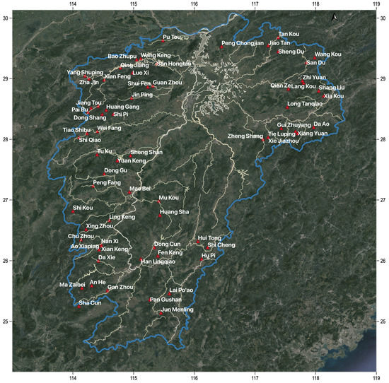
Figure 5.
Distribution of 69 hydrological stations in Jiangxi Province.
We conduct two groups of experiments. The first group of experiments is to construct clustering collectives, including several groups of comparative experiments. The second group of experiments is to carry out cluster fusion, including the construction of similarity matrix and similarity analysis.
Experiment 1: Construct Clustering Collectives
(1) Comparison of and
First, we generate clustering groups by the traditional clustering ensemble generation algorithm based on and , aiming to illustrate the superiority of in the small and medium watershed datasets.
The specific content is to call and multiple times on the input data set to obtain multiple clustering results. These clustering results are cluster members, which together form a clustering group. Then, the obtained clustering ensemble use evaluation indexes are calculated and compared. Considering that and will result in different results due to the random selection of the initial center point, the comparison is made here by averaging after multiple experiments. The specific parameters of the algorithm are as follows:
Input data: data collection of small and medium watersheds in Jiangxi Province;
Number of cluster members I: 10;
Experiment according to the above parameter settings, and the final result is shown in Table 2:
Table 2.
Comparison of clustering effects of traditional clustering construction algorithm based on K-Means and K-Medoids.
From the Table 2, we can see that when is used as the basic clustering algorithm, the clustering quality of the generated cluster members is better. It is because that the small- and medium-sized watershed data set used as the experimental input contains some noise points. We verify that the 27-dimensional small and medium watershed data set is reduced to a two-dimensional data set and then mapped to the map through MDS. For details, see Figure 6 below. This experiment can explain that the special performance of not affected by noise points improves the clustering quality of each cluster member in the clustering ensemble to some extent.
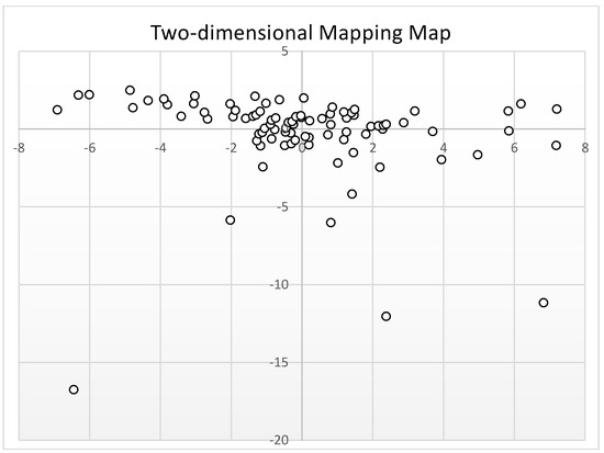
Figure 6.
Two-dimensional map of small and medium watershed data sets.
Since the center point of is selected from the points in the dataset, it can be seen from the Table 2 that the difference between cluster members finally generated by the algorithm is much smaller than that obtained by and the OCQ-NMI index obtained by the traditional algorithm based on is slightly lower than that based on . However, we need to find a method which can get results with high clustering quality and not affected by noise points to improve the clustering group quality. So, we choose algorithm. Aiming at the difference between cluster members, the method of constructing feature subsets by random sampling can effectively increase the difference among cluster members in the cluster group.
(2) Comparison of different clustering group construction algorithm
In the case of basic clustering using , the traditional clustering construction method, constructing clustering ensembles by random sampling (RS-CCE) and WRS-CCE are used to construct the clustering group, and several evaluation indicators are used to compare the clustering effects. The specific parameters are as follows:
Input data: . data collection of small and medium watersheds in Jiangxi Province;
Number of cluster members I: 10;
Number of iterations S: 1000;
Experiment according to the above parameter settings, and the final result is shown in Figure 7:
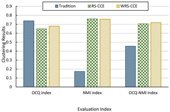
Figure 7.
Comparison of traditional construction method, constructing clustering ensembles by random sampling (RS-CCE) and clustering ensemble construction algorithm with weighted random sampling (WRS-CCE) clustering effect.
According to the experimental results in Figure 7, it can be seen that the comprehensive evaluation index of the clustering group constructed by the traditional construction method is very low because the difference index is too low, that is, the cluster members in the clustering group are too similar. It is because the method always takes the complete data set as input and cannot maintain the difference of the input data. The second reason is that the algorithmic nature of leads to a decrease in the difference. The RS-CCE will form a diversity feature subset by randomly selecting the feature indicators of the complete data set, and use it as an input data set to improve the difference between each cluster member in the cluster group. Although the quality of the cluster has decreased due to the lack of dimensions, the comprehensive quality of the clustering ensemble has been greatly improved from the comprehensive indicators. However, the RS-CCE randomly selects the feature subsets, so it is difficult to guarantee the stability of the clustering ensemble quality. The clustering collective generated by the WRS-CCE algorithm in this paper is slightly higher than the clustering group generated by the RS-CCE algorithm, but the difference is slightly lower. The reason is that WRS reduces the probability of selecting feature indicators which have bad effects on clustering and ensures the stability of cluster member quality. However, it also reduces the diversity of feature subsets and the differences between cluster members.
It can be seen from Figure 8 that the comprehensive index of the clustering ensemble generated by the RS-CCE algorithm will generate many peaks, and the fluctuations are very large. After iterations are repeated many times, it may still be in an unstable state. It is necessary to complete all iterations before ending the iteration, the clustering efficiency is low. The WRS-CCE algorithm achieves a large value and tends to be stable after the number of iterations reaches 100. The reason is that the algorithm quickly ends the iteration by dynamically updating the feature index weights and reducing the probability that the feature indicators that have bad effects on the cluster are selected. Therefore, it can be concluded that the clustering efficiency of WRS-CCE is much higher than that of RS-CCE.
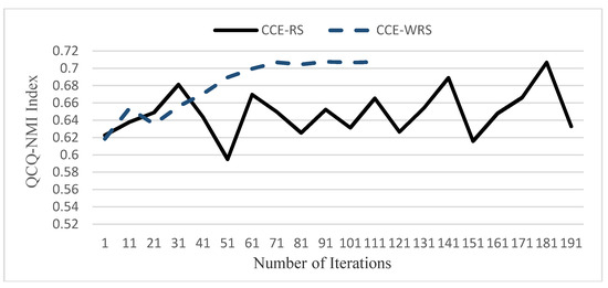
Figure 8.
Comparison of clustering efficiency between RS-CCE and WRS-CCE algorithms.
Experiment 2: Carry Out Clustering Fusion
(1) Comparison of different similarity matrix
This experiment processes the clustering groups based on the small- and medium-sized watershed dataset and generates the clustering cross-correlation matrix and CTS matrix respectively. It is intended to illustrate that the CTS matrix can reflect the similarities between data points to a greater extent than the cross-correlation matrix. The specific parameters of the experiment are as follows:
Input data: use the clustering groups based on the small and medium watershed data set of Jiangxi Province in Experiment 1;
The cross-correlation degree of the input data is calculated to obtain the cross-correlation matrix of the clustering ensemble. The partial results of the matrix are shown in Table 3:
Table 3.
Cross-correlation matrix obtained by clustering collectively based on the data set of small and medium watersheds in Jiangxi Province.
Input data: clustering groups based on the data set of small- and medium-sized watersheds in Jiangxi Province;
The input data is calculated by using the WCT algorithm to obtain the CTS matrix of the cluster. The partial results of the matrix are shown in Table 4:
Table 4.
Clustering Connected Triple Similarity (CTS) matrix based on small and medium watershed dataset.
According to the experimental results, it can be compared that the values in the CTS matrix are all larger than the values in the cross-correlation matrix, so that it can be verified that the CTS matrix does find the hidden relationship between the data points, that is, the degree of similarity between the data points is enhanced. Therefore, this paper chooses CTS matrix as the clustering similarity matrix and uses it as the input matrix of SC-FCM clustering fusion algorithm.
(2) Comparison of different clustering fusion algorithm
The experiment was carried out by direct FCM clustering experiment and SC-FCM clustering fusion experiment, and the results of two clustering experiments were analyzed to show that clustering integration can be more accurate than direct clustering method. It can find similar watersheds accurately in the design basin, make specific comparisons and analysis of the similarity of the basin. The specific parameters of the experiment are as follows:
Input data: data collection of small and medium watersheds in Jiangxi Province;
According to the above input data, the experiment is directly performed using the FCM clustering algorithm, and the final results are shown in Table 5:
Table 5.
Clustering results after direct FCM clustering (C represents Cluster).
Input data: use the CTS matrix obtained in above experiment;
According to the above input data, the SC-FCM clustering fusion algorithm was used for the experiment. The final results are shown in Table 6:
Table 6.
Clustering results after SC-FCM clustering fusion (C represents Cluster).
According to some data in Table 5 and Table 6, it can be seen that among the clustering results directly using FCM clustering, Mukou Station and Xianfeng Station have a high degree of membership belong to the same cluster (cluster 7), while the Sandu station has a low degree of membership in cluster 7. Among the clustering results after SC-FCM clustering, Mukou Station, Xianfeng Station, and Sandu Station belong to the same cluster (cluster 2), which means that Mukou Station, Xianfeng Station, and Sandu Station are likely to be similar.
In the literature [11], Fan Mengge proposed that if the two-year maximum flood peak and flood volume of the two stations are within 10%, they can basically be considered similar. Therefore, this paper uses this method of multi-year peak and flood comparison analysis to verify the similar situation with Mukou Station, Xianfeng Station and Sandu Station. Table 7 shows the comparison of the maximum flood peak flow and the maximum floods in 1, 3, 6, and 12 h of Mukou, Xianfeng, and Sandu stations.
Table 7.
Comparison of flood amount analysis.
It can be concluded from the above table that the gap between the flood peak and the flood volume of Sandu Station and Mukou Station is similar to that of Xianfeng Station and Mukou Station, almost within 10%. Therefore, it can be considered that Sandu Station and Mukou Station are similar, that is, the watershed where Sandu Station is located is also a similar watershed in the basin where Mukou Station is located, which proves that the similarity analysis of small and medium watersheds based on clustering integration can more accurately find similar watersheds in the design basin.
Secondly, the gap between the Sandu Station and the Mukou Station is much larger than that between the Xianfeng Station and the Mukou Station. Therefore, it can be considered that the basin where Mukou Station is located is more similar to the basin where Xianfeng Station is located. This conclusion is consistent with the case where the membership degree of Xianfeng Station is greater than that of Sandu Station in Table 6.
Figure 9 is the result of 69 small- and medium-sized watersheds similarity analysis based on clustering ensemble, and stations with the same color and shape are similar. The clustering integration method proposed in this paper can directly and effectively find out more similar basins.
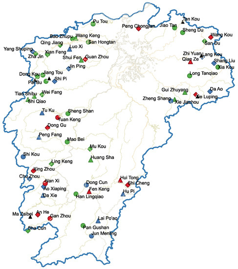
Figure 9.
The clustering results of clustering ensemble model.
5. Conclusions
Based on the characteristics of small- and medium-sized watershed and the theory of clustering ensemble, this paper studies the clustering ensemble model on the similarity analysis of small- and medium-sized watershed emphatically.
First, according to the characteristics of small- and medium-sized watershed data and OCQ-NMI comprehensive evaluation index, an iterative clustering collective construction algorithm based on weighted random sampling is proposed. The algorithm is applied to the pre-processed data sets of small- and medium-sized watersheds to construct clusters with high clustering quality and diversity.
Then, the consistency function is designed for the small- and medium-sized watershed data sets. The CTS matrix of clustering group is constructed by WCT algorithm, and then the matrix is clustered and fused by SC-FCM Clustering Fusion algorithm. Finally, the final clustering result is obtained, and the similarity analysis of small- and medium-sized watersheds is made according to the result.
Although some achievements have been made, there are still many problems to be solved. One problem is that the model proposed in this paper needs a lot of parameters. The selection of these parameters has not found a perfect algorithm to calculate the optimal value. It also needs continuous experiments and verification in the later period. In addition, the clustering ensemble algorithm designed in this paper only tests and verifies the data of small- and medium-sized watersheds. How to apply this algorithm to other levels of watersheds is the focus of future research.
Supplementary Materials
The following are available online at https://www.mdpi.com/2073-4441/12/1/69/s1, Algorithm S1: WRS Algorithm, Algorithm S2: getClusterK(D), Algorithm S3: kMediods(D), Algorithm S4: get SWT, Algorithm S5: getS (Data Points), Algorithm S6: getS (Data Sets).
Author Contributions
Conceptualization, Q.Z. and Y.L.; data curation, Q.Z.; formal analysis, Q.Z.; funding acquisition, Y.Z. and D.W.; investigation, Q.Z. and Y.Y.; methodology, Q.Z. and Y.L.; project administration, Y.Z. and D.W.; resources, Y.Z. and D.W.; software, Q.Z.; supervision, D.W.; validation, Y.Y.; visualization, Q.Z. and Y.Y.; writing—original draft, Q.Z. and Y.L.; writing—review and editing, Y.Z., D.W. and Y.Y. All authors have read and agreed to the published version of the manuscript.
Funding
This research has been supported by the National Key Research and Development Program of China (No. 2018YFC1508100), the National Key Research and Development Program of China (Nos.2018YFC0407900) and the CSC Scholarship.
Acknowledgments
In this section you can acknowledge any support given which is not covered by the author contribution or funding sections. This may include administrative and technical support, or donations in kind (e.g., materials used for experiments).
Conflicts of Interest
The authors declare no conflict of interest.
References
- Lei, J. Research on Flood Forecasting and Early Warning System for Small and Medium Watersheds. Master’s Thesis, Zhengzhou University, Zhengzhou, China, 2014. [Google Scholar]
- Wensheng, W.; Yueqing, L. Selection method of watershed area in waterless literature. J. Chengdu Univ. Technol. 2015, 18, 7–10. [Google Scholar]
- Wood, E.F.; Hebson, C.S. On hydrologic similarity: 1. Derivation of the dimensionless flood frequency curve. Water Resour. Res. 1986, 22, 1549–1554. [Google Scholar] [CrossRef]
- Merz, R.; Blöschl, G. Regionalisation of catchment model parameters. J. Hydrol. 2004, 287, 95–123. [Google Scholar] [CrossRef]
- Young, A.R. Stream flow simulation within UK ungauged catchments using a daily rainfall-runoff model. J. Hydrol. 2006, 320, 155–172. [Google Scholar] [CrossRef]
- Zhang, Y.; Chiew, F.H. Relative merits of different methods for runoff predictions in ungauged catchments. Water Resour. Res. 2009, 45. [Google Scholar] [CrossRef]
- Chen, S. Fuzzy Model and Method for Choosing Analogy Basins. Adv. Water Sci. 1993, 4, 288–293. [Google Scholar]
- Yaya, S.; Zheng, Z.; Zhengping, Z. Study on optimization of analogical watershed based on fuzzy weighted pattern recognition model. Yangtze River 2014, 21, 54–57. [Google Scholar]
- Ming, Z.; Guizuo, W.; Yanxi, Z. Study on maximum entropy optimization model for catchments with hydrological similarity. Water Resour. Hydropower Eng. 2012, 2, 14–16. [Google Scholar]
- Yusong, L.; Weimin, B.; Qian, L. Research on watershed clustering based on principal component analysis. Hydropower Sci. 2012, 3, 23–26. [Google Scholar]
- Mengge, F.; Jiufu, L. Hydrological similar watershed based on clustering analysis. J. Water Resour. Hydropower Eng. 2015, 4, 106–111. [Google Scholar]
- Xiaoming, Z. Research on Several Problems of Watershed Hydrological Scale. Ph.D. Thesis, Hohai University, Nanjing, China, 2006. [Google Scholar]
- Weizhen, Z.; Chunhuang, L.; Fangyu, L. Evaluation Method of Clustering Quality. Comput. Eng. 2005, 20, 10–12. [Google Scholar]
- Yan, Y.; Fan, Y.; Mohamed, K. Review of clustering effectiveness evaluation. J. Comput. Appl. 2008, 6, 1630–1632. [Google Scholar]
- Huilan, L. Research on Key Technologies of Clustering Integration. Ph.D. Thesis, Zhejiang University, Hangzhou, China, 2007. [Google Scholar]
- Strehl, A.; Ghosh, J. Cluster ensembles—A knowledge reuse framework for combining multiple partitions. J. Mach. Learn. Res. 2002, 3, 583–617. [Google Scholar]
- Fern, X.Z.; Brodley, C.E. Random projection for high dimensional data clustering: A cluster ensemble approach. In Proceedings of the Twentieth International Conference on Machine Learning (ICML-03), Washington, DC, USA, 21–24 August 2003; AAAI Press: Palo Alto, CA, USA, 2003. [Google Scholar]
- Von Luxburg, U. A tutorial on spectral clustering. Stat. Comput. 2007, 17, 395–416. [Google Scholar] [CrossRef]
- Dunn, J.C. A fuzzy relative of the ISODATA process and its use in detecting compact well-separated clusters. J. Cybern. 1973, 3, 32–57. [Google Scholar] [CrossRef]
- Bezdek, J.C. Pattern Recognition with Fuzzy Objective Function Algorithms; Springer Science & Business Media: Berlin, Germany, 2013. [Google Scholar]
- Bingyi, L. Clustering Integration Algorithm and Application Research. Master’s Thesis, Nanjing University of Science and Technology, Nanjing, China, 2012. [Google Scholar]
- Caliński, T.; Harabasz, J. A dendrite method for cluster analysis. Commun. Stat.-Theory Methods 1974, 3, 1–27. [Google Scholar] [CrossRef]
- Davies, D.L.; Bouldin, D.W. A cluster separation measure. IEEE Trans. Pattern Anal. Mach. Intell. 1979, 2, 224–227. [Google Scholar] [CrossRef]
- Iam-On, N.; Boongoen, T.; Garrett, S. Refining Pairwise Similarity Matrix for Cluster Ensemble Problem with Cluster Relations; Springer: Berlin, Germany, 2008. [Google Scholar]
- Xiaowei, C.; Guanzhong, D.; Libin, Y. Overview of Spectral Clustering Algorithms. Comput. Sci. 2008, 07, 14–18. [Google Scholar]
© 2019 by the authors. Licensee MDPI, Basel, Switzerland. This article is an open access article distributed under the terms and conditions of the Creative Commons Attribution (CC BY) license (http://creativecommons.org/licenses/by/4.0/).