Quantitative Evaluation of Groundwater–Surface Water Interactions: Application of Cumulative Exchange Fluxes Method

Abstract
1. Introduction
2. Materials and Methods
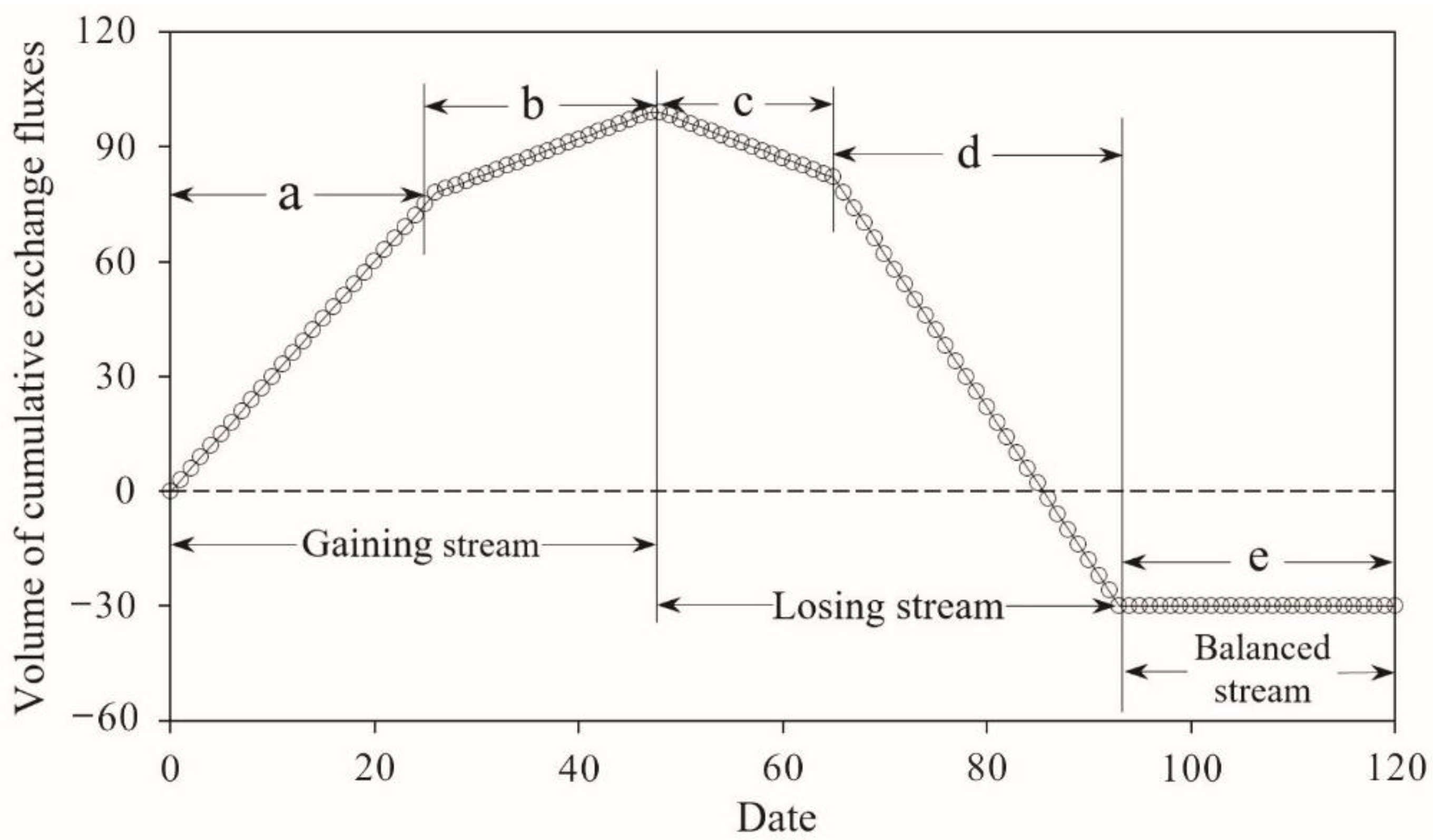
2.1. Theory of Cumulative Exchange Fluxes Method
2.2. Study Area
2.3. Data Collection
3. Results and Discussion
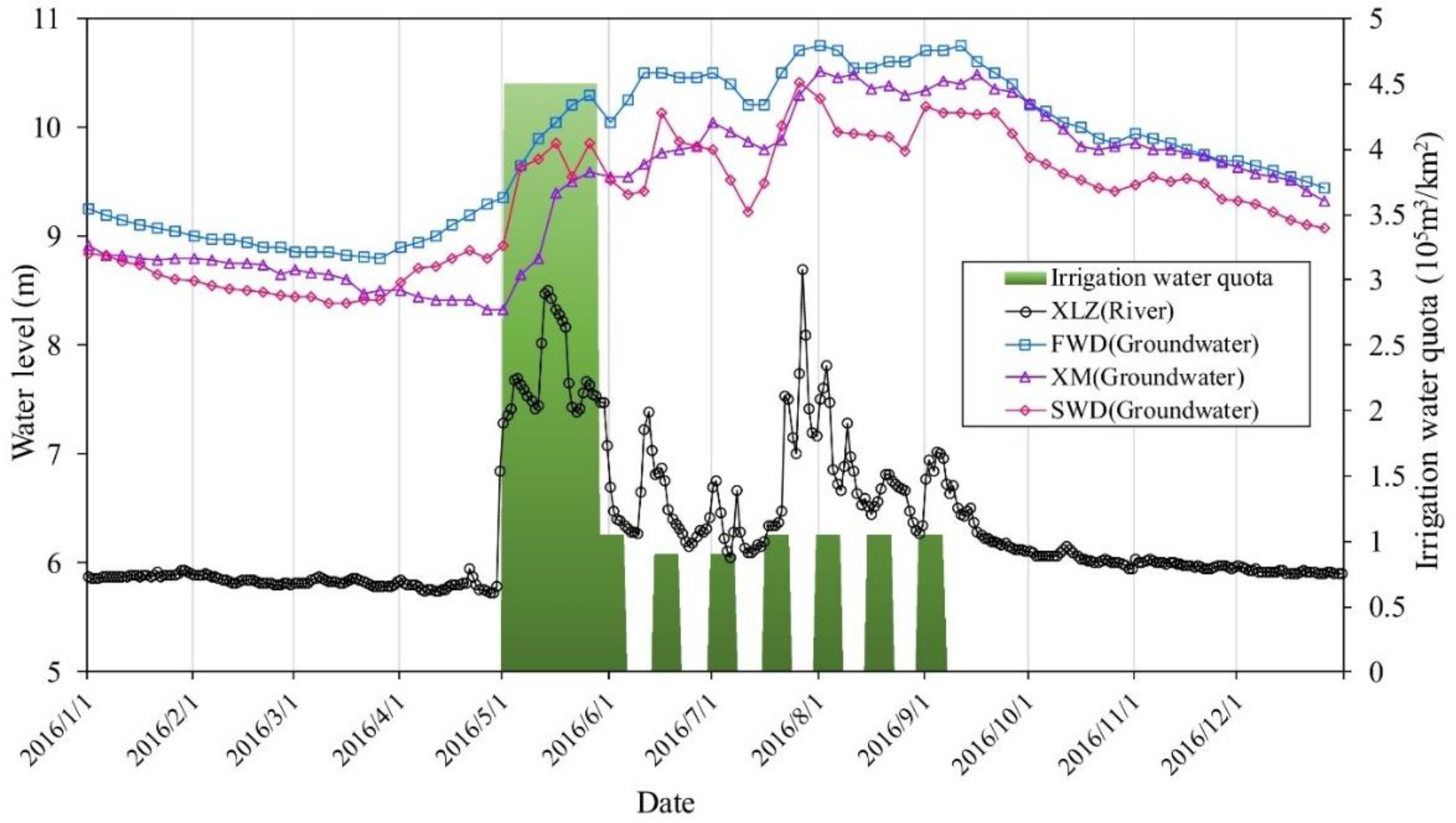
3.1. Calculation of the Exchange Fluxes in 2016
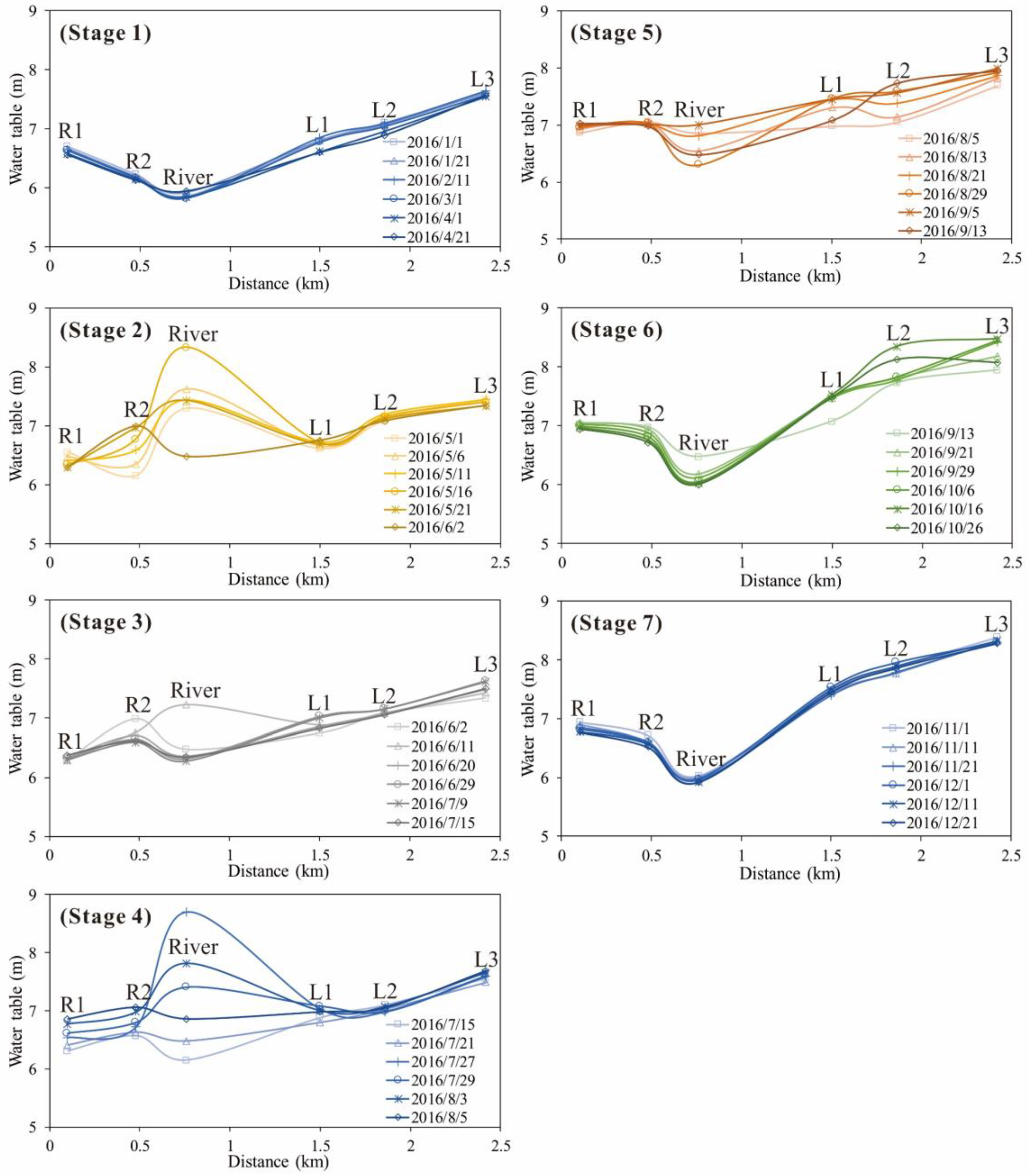
3.2. Analysis of the Exchange Fluxes in 2016
3.3. Verification of Method’s Accuracy
3.4. Error Analysis of Exchange Fluxes Calculation
3.5. The Applicability of Cumulative Exchange Fluxes Method
3.6. Support for Other Research Methods
4. Conclusions
Author Contributions
Funding
Conflicts of Interest
References
- Jolly, I.; Mcewan, K.; Holland, K. A review of groundwater-surface water interactions in arid/semi-arid wetlands and the consequences of salinity for wetland ecology. Ecohydrology 2010, 1, 43–58. [Google Scholar] [CrossRef]
- Kalbus, E.; Reinstorf, F.; Schirmer, M. Measuring methods for groundwater-surface water interactions: A review. Hydrol. Earth Syst. Sci. Discuss. 2006, 10, 873–887. [Google Scholar] [CrossRef]
- Sophocleous, M. Interactions between groundwater and surface water: The state of the science. Hydrogeol. J. 2002, 10, 52–67. [Google Scholar] [CrossRef]
- Martinez, J.L.; Raiber, M.; Cox, M.E. Assessment of groundwater-surface water interaction using long-term hydrochemical data and isotope hydrology: Headwaters of the Condamine River, Southeast Queensland, Australia. Sci. Total Environ. 2015, 536, 499–516. [Google Scholar] [CrossRef] [PubMed]
- Li, M.; Liang, X.; Xiao, C.; Cao, Y.; Hu, S. Hydrochemical Evolution of Groundwater in a Typical Semi-Arid Groundwater Storage Basin Using a Zoning Model. Water 2019, 11, 1334. [Google Scholar] [CrossRef]
- Lambs, L. Interactions between groundwater and surface water at river banks and the confluence of rivers. J. Hydrol. 2004, 288, 312–326. [Google Scholar] [CrossRef]
- Kumar, M.; Ramanathan, A.; Keshari, A.K. Understanding the extent of interactions between groundwater and surface water through major ion chemistry and multivariate statistical techniques. Hydrol. Process. 2010, 23, 297–310. [Google Scholar] [CrossRef]
- Winter, T.C. Recent Advances in Understanding the Interaction of Groundwater and Surface Water. Rev. Geophys. 1995, 33, 985–994. [Google Scholar] [CrossRef]
- Ji, C.M.; Hou, J.Y.; Wang, Z.X. Groundwater Development in the World and Guidelines for International Cooperation; Seismological Press: Beijing, China, 1996. (In Chinese) [Google Scholar]
- Werner, A.D.; Simmons, C.T. Impact of sea-level rise on sea water intrusion in coastal aquifers. Groundwater 2010, 47, 197–204. [Google Scholar] [CrossRef]
- Devito, K.J.; Hill, A.R.; Roulet, N. Groundwater-surface water interactions in headwater forested wetlands of the Canadian Shield. J. Hydrol. 1996, 181, 127–147. [Google Scholar] [CrossRef]
- Hu, L.T.; Chen, C.X.; Jiao, J.J.; Wang, Z.J. Simulated groundwater interaction with rivers and springs in the Heihe river basin. Hydrol. Process. 2010, 21, 2794–2806. [Google Scholar] [CrossRef]
- Mccallum, A.M.; Andersen, M.S.; Giambastiani, B.M.S.; Kelly, B.F.J.; Ian Acworth, R. River-aquifer interactions in a semi-arid environment stressed by groundwater abstraction. Hydrol. Process. 2013, 27, 1072–1085. [Google Scholar] [CrossRef]
- Weissteiner, C.J.; Pistocchi, A.; Marinov, D.; Bouraoui, F.; Sala, S. An indicator to map diffuse chemical river pollution considering buffer capacity of riparian vegetation—A pan-European case study on pesticides. Sci. Total Environ. 2014, 484, 64–73. [Google Scholar] [CrossRef] [PubMed]
- Knight, R.R.; Gain, W.S.; Wolfe, W.J. Modelling ecological flow regime: An example from the Tennessee and Cumberland River basins. Ecohydrology 2012, 5, 613–627. [Google Scholar] [CrossRef]
- Jiang, Y.; Wu, Y.; Groves, C.; Yuan, D.; Kambesis, P. Natural and anthropogenic factors affecting the groundwater quality in the Nandong karst underground river system in Yunan, China. J. Contam. Hydrol. 2009, 109, 49–61. [Google Scholar] [CrossRef]
- Murdoch, L.C.; Kelly, S.E. Factors Affecting the Performance of Conventional Seepage Meters. Water Resour. Res. 2003, 39, 1163. [Google Scholar] [CrossRef]
- Anderson, M.P. Heat as a ground water tracer. Groundwater 2010, 43, 951–968. [Google Scholar] [CrossRef]
- Barthel, R.; Banzhaf, S. Groundwater and Surface Water Interaction at the Regional-scale—A Review with Focus on Regional Integrated Models. Water Resour. Manag. 2016, 30, 1–32. [Google Scholar] [CrossRef]
- Constantz, J.; Cox, M.H.; Su, G.W. Comparison of heat and bromide as ground water tracers near streams. Groundwater 2010, 41, 647–656. [Google Scholar] [CrossRef]
- Zhang, Y.; Wang, D.; Wang, X.; Meng, W. Effects of reservoir construction on flow regimes in the Taizi river. Res. Environ. Sci. 2012, 25, 363–371. [Google Scholar]
- De Serio, F.; Mossa, M. Analysis of mean velocity and turbulence measurements with ADCPs. Adv. Water Resour. 2015, 81, 172–185. [Google Scholar] [CrossRef]
- Fu, G.; Liu, C.; Chen, S.; Hong, J. Investigating the conversion coefficients for free water surface evaporation of different evaporation pans. Hydrol. Process. 2014, 18, 2247–2262. [Google Scholar] [CrossRef]
- Lobo, J.; Costa, P.M.; Caeiro, S.; Martins, M.; Ferreira, A.M.; Caetano, M.; Cesário, R.; Vale, C.; Costa, M.H. Reconstruction of a Daily Large-Pan Evaporation Dataset over China. J. Appl. Meteorol. Clim. 2011, 51, 1265–1275. [Google Scholar]
- Liaoning Provincial Department of Water Resources. Water Resources in Liaoning Provence; Liaoning Science and Techinology Publishing House: Shenyang, China, 2005. (In Chinese)
- Sriwongsitanon, N.; Taesombat, W. Effects of land cover on runoff coefficient. J. Hydrol. 2011, 410, 226–238. [Google Scholar] [CrossRef]


| Flux and Other Data | Method of Quantification | |
|---|---|---|
| Gauged Qdown, Qup and Qt | Daily gauging station data | |
| Ungauged, Qc | Estimated based on runoff coefficients | |
| Qd (for example, canal diversions) | Daily operational gauge measurements | |
| Qo | Change in weir storage | Daily operational weir volume measurements |
| River pumping | Daily operational estimates | |
| Area of river surface | Simply mean river width multiplied by length or Landsat-based image interpretation | |
| Precipitation | Daily mean precipitation from nearest climate station | |
| Evaporation | Daily mean evaporation from nearest climate station | |
| Runoff coefficient | Estimated from regional hydrological studies that have passed acceptance | |
| Month | April | May | June | July | August | September | October | November | December–March |
|---|---|---|---|---|---|---|---|---|---|
| Conversion coefficient C | 0.56 | 0.56 | 0.57 | 0.59 | 0.60 | 0.63 | 0.58 | 0.57 | 0.5 |
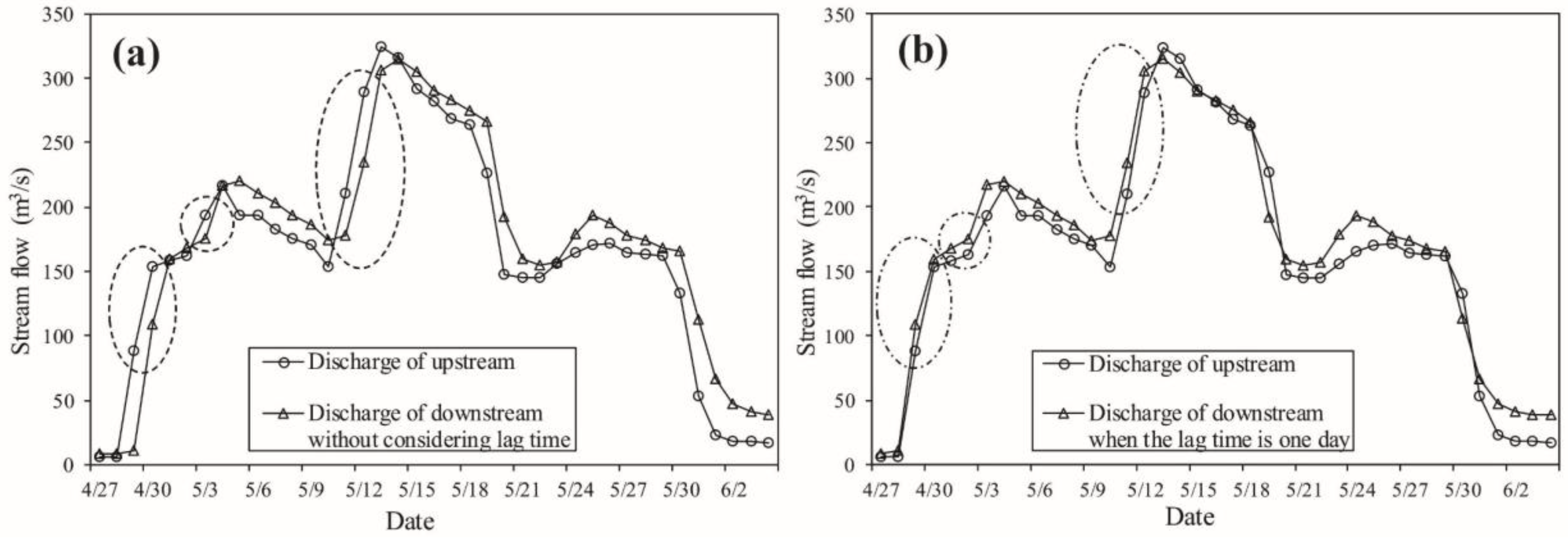
| Date in 2016 | 4/19 | 4/30 | 5/13 | 6/10 | 7/1 | 7/22 | 7/26 | 8/2 | 8/8 | 8/19 |
|---|---|---|---|---|---|---|---|---|---|---|
| Peak flow at upstream (m3/s) | 33.52 | 153.57 | 324.3 | 118.91 | 55.4 | 137.8 | 258 | 202.2 | 126.2 | 71.89 |
| Peak flow at downstream (m3/s) | 19.6 | 160 | 315 | 154 | 86 | 185 | 347 | 216 | 144 | 86.5 |
| Lag time (day) | 2 | 1 | 1 | 2 | 1 | 0 | 1 | 1 | 1 | 1 |
| State | Period | Duration Time (day) | Amount of Exchange Fluxes (107 m3) | GW-SW Interaction | Exchange Rate (105 m3/day) |
|---|---|---|---|---|---|
| 1 | 1.1–4.27 | 117 | 3.67 | Gaining stream | 3.13 |
| 2 | 4.27–6.2 | 36 | 0.13 | Mainly gaining stream, sometimes losing stream | 0.36 |
| 3 | 6.2–7.19 | 47 | 5.28 | Gaining stream | 11.24 |
| 4 | 7.19–8.5 | 17 | 0.46 | Mainly gaining stream, sometimes losing stream | 2.69 |
| 5 | 8.5–9.13 | 39 | 6.75 | Gaining stream | 17.32 |
| 6 | 9.13–10.31 | 48 | 3.11 | Gaining stream | 6.48 |
| 7 | 10.31–12.31 | 61 | 2.29 | Gaining stream | 3.76 |
| Sum | 1.1–12.31 | 365 | 21.69 | Gaining stream | 5.94 |
© 2020 by the authors. Licensee MDPI, Basel, Switzerland. This article is an open access article distributed under the terms and conditions of the Creative Commons Attribution (CC BY) license (http://creativecommons.org/licenses/by/4.0/).
Share and Cite
Li, M.; Liang, X.; Xiao, C.; Cao, Y. Quantitative Evaluation of Groundwater–Surface Water Interactions: Application of Cumulative Exchange Fluxes Method. Water 2020, 12, 259. https://doi.org/10.3390/w12010259
Li M, Liang X, Xiao C, Cao Y. Quantitative Evaluation of Groundwater–Surface Water Interactions: Application of Cumulative Exchange Fluxes Method. Water. 2020; 12(1):259. https://doi.org/10.3390/w12010259
Chicago/Turabian StyleLi, Mingqian, Xiujuan Liang, Changlai Xiao, and Yuqing Cao. 2020. "Quantitative Evaluation of Groundwater–Surface Water Interactions: Application of Cumulative Exchange Fluxes Method" Water 12, no. 1: 259. https://doi.org/10.3390/w12010259
APA StyleLi, M., Liang, X., Xiao, C., & Cao, Y. (2020). Quantitative Evaluation of Groundwater–Surface Water Interactions: Application of Cumulative Exchange Fluxes Method. Water, 12(1), 259. https://doi.org/10.3390/w12010259