Article

A Continuous Drought Probability Monitoring System, CDPMS, Based on Copulas

by
João Dehon Pontes Filho
1,
Maria Manuela Portela
2,*,
Ticiana Marinho de Carvalho Studart
1 and
Francisco de Assis Souza Filho
1
1
Hydraulic and Environmental Engineering Department (DEHA), Federal University of Ceará, 60020-181 Fortaleza-CE, Brazil
2
Civil Engineering Research and Innovation for Sustainability (CERIS), Instituto Superior Tecnico (IST), University of Lisbon, 1649-004 Lisboa, Portugal
*
Author to whom correspondence should be addressed.
Water 2019, 11(9), 1925; https://doi.org/10.3390/w11091925
Submission received: 29 July 2019 / Revised: 24 August 2019 / Accepted: 11 September 2019 / Published: 14 September 2019
(This article belongs to the Special Issue Management of Hydrological Extremes: Floods and Droughts)

Abstract

:
The standardized precipitation index (SPI), is one of the most used drought indices. However, it is difficult to use to monitor the ongoing drought characteristics because it cannot be expeditiously related to precipitation deficits. It also does not provide information regarding the drought probability nor the temporal evolution of the droughts. By assigning the SPI to drought-triggering precipitation thresholds, a copula-based continuous drought probability monitoring system (CDPMS), was developed aiming to monitor the probability of having a drought as the rainy season advances. In fact, in climates with very pronounced rainy seasonality, the absence of precipitation during the rainy season is the fundamental cause of droughts. After presenting the CDPMS, we describe its application to Mainland Portugal and demonstrate that the system has an increased capability of anticipating drought probability by the end of the rainy season as new precipitation records are collected. The good performance of the system results from the ability of the copula to model complex dependence structures as those existing between precipitations at different time intervals. CDPMS is an innovative and user-friendly tool to monitor precipitation and, consequently, the drought probability, allowing the user to anticipate mitigation and adaptation measures, or even to issue alerts.

1. Introduction

Drought is a natural phenomenon without a clear onset which makes it difficult to recognize. It is the world’s costliest natural disaster and can provide impacts in a global perspective, not restricted to places with low average precipitation amounts [1,2,3]. In Europe, the total cost of drought damages recorded from 1976 to 2006 amounted to 100 billion € [4]. Therefore, the continuous monitoring of the probability of drought events is crucial to deploy short term emergency measures and to mitigate the social, environmental and economic costs and losses associated with those events.
Considerable disagreement exists about the definition of drought. However, all the definitions relate the event to below-average precipitation over a period of time. If the event persists long enough, it can progressively affect soil moisture, water resources, and, consequently, economic and social development. According to its impacts, the droughts can be classified into four categories: meteorological, agricultural, hydrological, and socioeconomic [1,5].
Drought indices are the most suitable tool for drought monitoring and evaluation. Many different indices have been proposed in the last decades. Among the hydrological variables adopted to detect and characterize drought occurrences, precipitation is the most widely used, not only due to its intrinsic link with the phenomenon and its consequences but also because precipitation is widely monitored and there are relatively long historical records.
In 2009, the World Meteorological Organization (WMO) recommended the standardized precipitation index (SPI) [6] to monitor meteorological drought conditions. Since then, the SPI is used worldwide to detect anomalous precipitation over different time scales. The SPI has the advantage of being independent of the magnitude of the mean precipitation, because it is a standardized index, and hence, able to compare droughts in different climatic zones. However, because it provides a standardized numerical value, it is difficult to connect it expeditiously to precipitation deficits, and, consequently, to use it to recognize or to predict drought events.
The droughts have traditionally been studied in a univariate context, mostly aiming at identifying and describing their occurrences. However, as many of the hydrological phenomena, they are characterized by multiple aspects some of them expectably correlated. Since a univariate approach ignores the dependence structure among those aspects, it may result in a poorer representation of the phenomenon.
Before copulas approach, some multivariate techniques were introduced in hydrological studies, such as in the case of the analysis of floods, droughts, and storms. Those techniques contribute to improving the accuracy of the estimates and provide information about the dependence structure among the characteristics. Most of them used bivariate probability distributions, such as bivariate gaussian, exponential, gamma, and extreme value distributions. The disadvantage of such approaches is that the marginals must have the same probability distribution and extensions to more than the bivariate case are not clear [7,8]. However, copulas can overcome such difficulties [9]. The advantages of using copulas to model complex relationships among variables are (1) flexibility in choosing arbitrary marginals and structures of dependence, (2) capability to model more than two variables, and (3) splitting of marginal and dependence structure analysis [7,8,10,11].
Multiple dependent random variables need more advanced and complex copulas than the common ones that are applied to the bivariate case. An example is the vine-copulas, which are able of coupling multiple variables into a pair-to-pair manner [12].
The application of copulas in hydrology has gained some relevance in the last decades. Regarding drought analysis, one of the main uses of copulas is to model the frequency analysis, combining different characteristics of the drought events (e.g. intensity, duration, magnitude, and spatial distribution) [13,14,15,16,17]. Another important use of copulas is its application to the joint modeling of drought indexes of different drought categories, such as meteorological, hydrological and agricultural [18,19,20].
In climatic regions like Mainland Portugal, insufficient precipitation during the short-duration and well-defined rainy season is the main trigger of the drought events. An innovative use of copulas could be its application in a multivariate context to monitor the evolution of the drought probability during that season, based on the continuous updating of precipitation that already occurred and the one that needs to occur, so that there is (or not) a drought by the end of the rainy season (a typical conditional probability problem). The conditional probability theory coupled with copulas is frequently used in hydrological applications to analyze multivariate dependence [17,21,22] and will be applied in this study.
Aiming at exploring copula’s forecasting capabilities in a drought monitoring context, the concept of a precipitation threshold for drought recognition developed by [23,24,25] was used. In each rain gauge, if the cumulative precipitation in a given timespan falls below the precipitation threshold for that timespan, a drought with a severity (from moderate to extreme), defined by the threshold, will occur. Figure 1 exemplifies the application to Mainland Portugal of the precipitation surface threshold concept applied to recognize moderate to extreme droughts from October to March (the rainy season). If in a certain location the precipitation registered falls below the value given by one of the maps, then the location experienced a drought, with the intensity given by the threshold to which the map relates.
The application of the precipitation threshold concept in the scope of the present study can be formulated as follows: for a season of N months to which the time scale of the SPI and the precipitation threshold, R N * , refer, let R n denote the observed precipitation in the first n months ( 1 n N ) and R N the total seasonal precipitation.
A drought will occur by the end of the N -month period if R n added to the (unknown) precipitation in the remaining ( N n ) months, R ( N n ) , is not enough to meet the threshold, R N * , i.e.,:
R n +   R ( N n ) R N * R N R N *
Consider, for example, the six-month season, N = 6, from October to March (during which most of the precipitation in Portugal falls) and, that at the end of December of a given year, an estimate of the probability of a moderate, severe or extreme drought occurrence is envisaged. Given the observed precipitation from October to December ( R n with n = 3), the problem to be addressed for each drought intensity can be stated as what is the probability the precipitation from January to March (still unknown) added to the precipitation from October to December being below the drought threshold? The solution is the drought probability given by the following equation:
P   ( R N R N * | R n ) P   ( R 6 R 6 * | R 3 )
By coupling a copulas approach with the precipitation threshold concept, the main objectives of this study were as follow: 1) to develop a methodology for a Continuous Drought Probability Monitoring System, CDPMS, 2) to evaluate the performance of CDPMS, and 3) to apply the CDPMS to a study area. To demonstrate the methodology, Mainland Portugal and its rainy season (from October to March) were selected. In Portugal, the precipitation regime is characterized by very pronounced seasonality, in average with 80% of the precipitation occurring from October to March, which makes it relevant to be able to anticipate if drought conditions are expected by the end of that period.

2. Materials and Methods

The development of the CDPMS was based on the stepwise approach described in Section 2.1.1, Section 2.1.2 and Section 2.1.3 and shown in Figure 2, steps (a) to (c). First, the drought threshold for a given time span or scale of the SPI, N , and drought severity is defined. After that, the copula candidates aiming at modeling the precipitation correlation structure are evaluated and those with best-fit are selected. Finally, the drought probability given by Equation (2) is computed. Having in mind that the goal of the CDPMS is to continuously monitor the probability of drought by the end of a N -month period, steps (b) and (c) are repeated from n = 1 to n = N − 1. The Leave-One-Out Cross-Validation (LOOCV) methodology (steps (b) and (c) repeated from x = 1 until the length x of time series) was used to evaluate the model performance using the Brier and the Brier Skill scores (d).
The CDPMS was applied to Mainland Portugal based on precipitation records at 45 rain gauges (described later in Section 3).

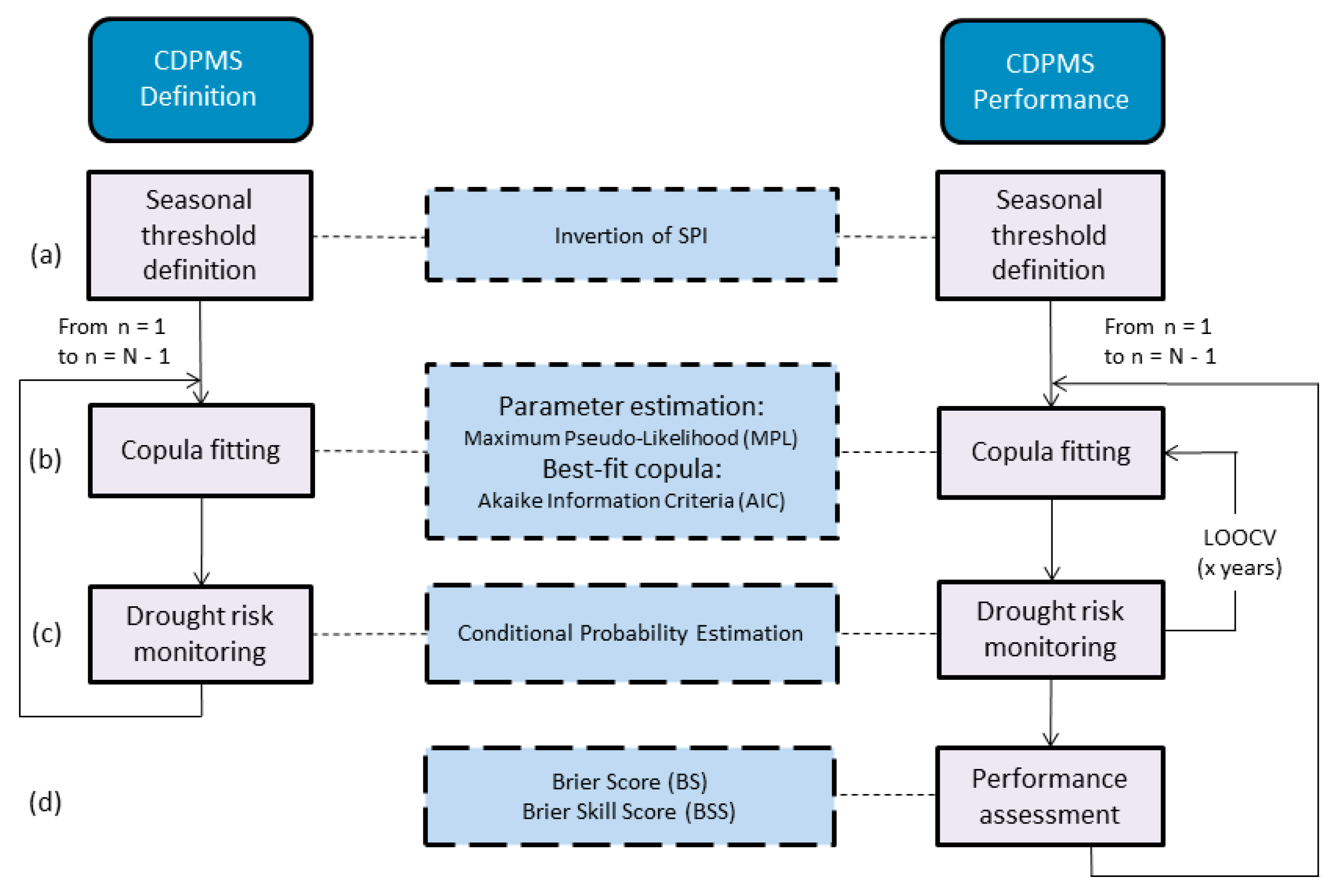
2.1. CDPMS Definition

2.1.1. Seasonal Threshold Definition

The precipitation in Mainland Portugal falls mainly from October (beginning of the hydrological year) to March, representing, on average, almost 70% and 85% of the annual precipitation in the North and South, respectively. Therefore, it was considered relevant to estimate the probability of drought occurrence by the end of the rainy season. The corresponding precipitation thresholds were obtained by inverting the SPI from October to March, SPI6, for each of the drought intensities proposed by Agnew [26] and presented in Table 1. For a given rain gauge and drought severity, the precipitation threshold, R N * , give the SPI value back to the precipitation field [23,24,25].

2.1.2. Copula Fitting

The analysis of the dependency structure between two or more random variables can be used to indicate predictive relationships among them. The most common method is to measure the linear relationship using the Pearson correlation coefficient. One of the main weaknesses of linear correlation is that it tends to detect only the degree of dependence despite its dependence structure.
The consideration of non-linear dependence is possible by applying a rank correlation coefficient such as Spearman rank correlation and Kendall’s Tau. The last coefficient is more used because its value indicates directly the probability of observing concordant or discordant pairs. There exists a relationship between the rank correlation coefficient and copula function that allows the use of copulas to study non-linear dependences.
According to Sklar’s theorem [27], if the random variables x1, …, xm follow a marginal probability distribution function F1(x1), …, Fm(xm), respectively, there exists a copula, C, that can join these marginal distribution functions in the form of a joint distribution function (Equation (3)),
H ( x 1 ,   x 2 ,   x m ) = C [ ( F 1 ( x 1 ) ,   F 2 ( x 2 ) , ,   F m ( x m ) =   C ( u 1 ,   u 2 ,   , u m )
where, Fk(xk) = uk for k = 1, ..., m, with uk ~ u(0,1) and C(u1, ..., um ) being the copula function.
Although copulas may be implemented in multiple dimensions only bivariate copulas were considered in the present study.
Different families of copulas have been described by Nelsen [27]. The families are commonly classified in four main groups: Meta-elliptical copulas (Gaussian and t Student), Archimedean copulas (Clayton, Gumbel, Frank, and Joe), Extreme value type (Gumbel, Husler-Reiss, Galambos, Tawn, and t-EV), and miscellaneous type (Plackett and Farlie–Gumbel–Morgenstern).
The Archimedean copulas are very popular for hydrological analyses as they allow modeling a great diversity of dependence structures, especially for dependent tail structures, and because of its accessible generation properties [8,14,28]. At higher orders, the use of Archimedean copulas is limited because their structure imposes restrictions related to dependence characteristics that are extremely difficult to satisfy for more than two variables [29]. Meta-Elliptical copulas, on the other hand, can model higher-order due to their simple structure that can better fit the complex dependence of multi-dimensional problems [9,30].
The parameters for the copulas families can be estimated either by the method of moments, inversion of Kendall’s Tau or by maximum likelihood estimation (MLE). The first method has the disadvantage of being applicable only to one-parameter copulas. As for the MLE method, two possibilities exist: The inference functions from margins (IFM) [31] or the maximum pseudo-likelihood method (MPL) [32]. How the transformation to [0,1] interval was made will dictate which is the best method, parametric for IFM and MPL for rank-based [33].
To model the dependence structure between the precipitation in a given sub-period of the rainy season and the seasonal precipitation itself, as is the case of the current application, the most popular Meta-Elliptical copulas (Gaussian and t Student), and Archimedean copulas (Clayton, Gumbel, and Frank) were tested as candidates. The copula formulation for each candidate family and its parameters’ interval are presented in Table 2. For each month of the rainy season, the bivariate model was constructed based on the two variables: precipitation in its initial n months ( R n ) and the total seasonal precipitation ( R N ).
The parameters θ for Archimedean copulas and ρ and v for Meta-Elliptical copulas, with v standing for the degrees of freedom (only needed for t Student copulas), were estimated for the candidate copulas. The MPL method was used as in [9]. This method was chosen because it can estimate both one and two parameters of the copula without requiring the establishment of the marginal distributions.
The Akaike Information Criterion (AIC) was applied to compare the bivariate copula models for the candidate families. The AIC method penalizes the models with the highest number of parameters, allowing to find the model with maximum explanatory power and fewer parameters, according to the parsimony principle.

2.1.3. Conditional Probability

The conditional probability theory associated with copulas is highly used in hydrological applications to analyze multivariate dependence [17,21,22] and can be expressed by Equation (4). Let two random variables X and Y with U 1 = Fx(x), U 2 = Fy(y) and u 1 and u 2 being specific values. The conditional distribution of X given Y = y is given by:
H ( X x   | Y = y ) = C θ ( U 1 | U 2 =   u 2 ) = u 2 C θ ( u 1 , u 2 )

2.2. CDPMS Performance Assessment

The CDPMS performance was measured by the Brier Score based on the previous computation of the probability of the coupled precipitation events for all the years with data but one (x − 1), according to the LOOCV. The validity of the probabilistic prediction was evaluated by the Brier Skill Score. In the LOOCV method, each of the x observed years is evaluated by removing one year of the time series, by fitting the model to the remaining x − 1 years, and by estimating the removed data [34]. The process is repeated x times to exclude any bias in performance verification. It is important to note that LOOCV is not part of CDPMS, as it was used only to assess the model’s performance, as shown in Figure 2. The model performance is compared against a random reference forecast.

2.2.1. Brier Score (BS)

The drought probability provided by the proposed copula-based model for each month can be analyzed using the Brier Score (BS), a verification measure of binary events (yes/no) that is used in multivariate models [35,36]. BS can mainly be regarded as the mean squared error between the probability of the drought prediction ( p i ), and a value of a binary variable associated with the observations ( o i ) by assigning 1, if the event occurs, and 0, if it does not, where x is the length of the time series. The BS takes values in the range 0 to 1, with 0 being a perfect prediction, according to [34]:
B S =   1 x i = 1 x ( p i o i ) 2

2.2.2. Brier Skill Score (BSS)

The Brier Skill Score (BSS) was used to evaluate the reliability of the probabilistic prediction (or skill). The score is calculated from the BS for the CDPMS (BSCDPMS) and from the BS for a reference forecast (BSREF) according to Equation (6), whose results range from −∞ to 1. BSS = 0 means no skill in comparison to the reference, and BSS = 1, perfect skill.
B S S = 1 B S C D P M S B S R E F
In the application carried out, the reference forecast selected for the evaluation of the prediction performance is the random probability of occurrence of a drought with a given intensity. Since this score was only applied to moderate droughts (SPI < −0.84, corresponding to the 20th percentile [26]) the p i for the BSREF was set equal to 0.20.

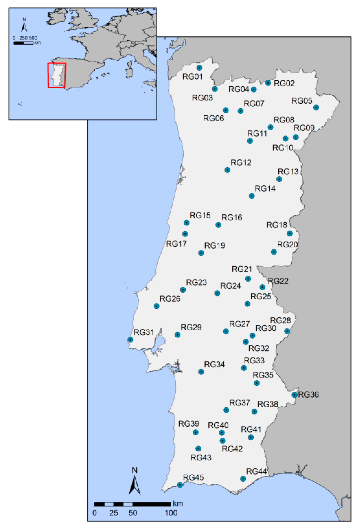
3. Precipitation Data

In order to construct a reliable bivariate statistical model for concurrent precipitation distributions, long historical continuous observations are needed. In the application presented herein, 45 rain gauges evenly distributed over mainland Portugal were selected (Figure 3, Table 3).
The monthly precipitation records were acquired by the Portuguese Environmental Agency, APA, and made available via the SNIRH database (Sistema Nacional de Informacão de Recursos Hídricos, http://snirh.pt), which has high data quality standards. The SNIRH is the main source of Portuguese hydrological and hydrometeorological data used by researchers and practitioners of water resources engineering and science.
Some of the precipitation series had missing values that were filled by applying an approach based on a linear regression analysis [37]. For each monthly gap in a given rain gauge, the approach identifies the candidate rain gauges that can be used for filling it. These gauges are next ranked according to the correlation coefficient between paired series for that month at the rain gauge with the gap and at each of the candidate rain gauges. The candidate rain gauge with higher correlation coefficient is next selected and used to fill the gap based on a linear regression model that is specific for each gap [37]. The length of the series after filling the missing values was x = 100 hydrological years, from 1918/1919 to 2017/2018.

4. CDPMS for Mainland Portugal: Definition and Performance

The following items describe the stepwise development and the performance assessment of the CDPMS developed to continuously monitor the drought probability over Mainland Portugal during the rainy season, based on the precipitation records at the 45 rain gauges of Figure 3. The application to a specific site is presented in Section 5.

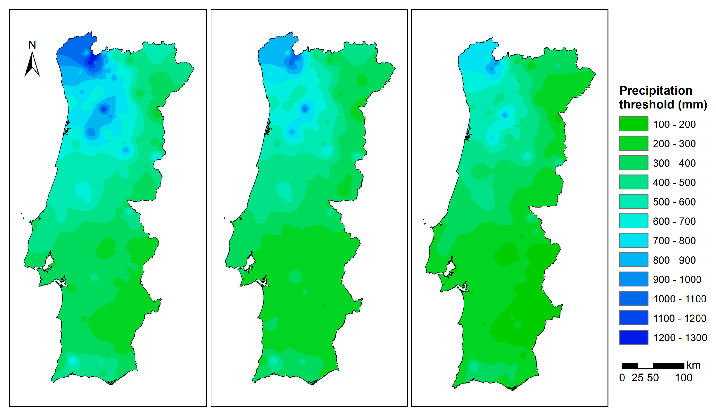
4.1. Precipitation Thresholds for Drought Recognition
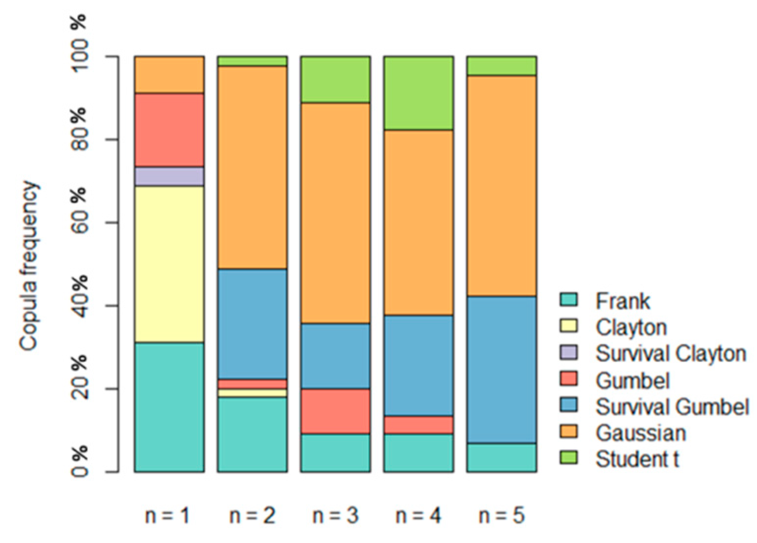
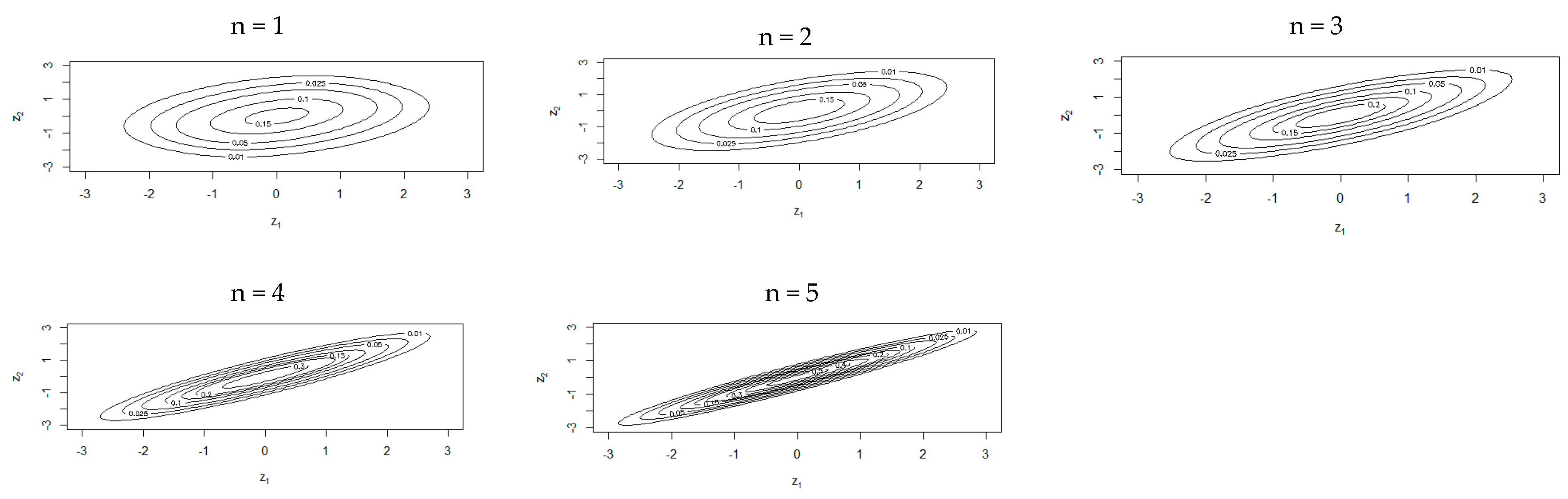
Table 4 presents the precipitation thresholds, R N * , in the 45 rain gauges obtained by inverting the SPI for the time span of 6 months (SPI6), from October to March, for the different drought intensities (moderate, severe and extreme). By the end of March, a drought with a given intensity occurs in a given rain gauge whenever the precipitation for the period is smaller than the precipitation threshold for that intensity.

4.2. Copula Fitting

In each rain gauge, the bivariate model was constructed by coupling the precipitation in the rainy season, R N for N = 6, with the precipitation in the initial n months of that season, R n (i.e., the precipitation in October, for n = 1, from October and November, for n = 2 and so on until n = 5, from October to February). The length of each coupled ( R N , R n ) series is equal to the length of the recording period (x = 100 years). The parameters were estimated by the MPL method, and the candidate copula families were selected based on the AIC.
For the 45 rain gauges, the frequency of the copula families chosen for each value of n is presented in Figure 4. Considering, for example, n = 1, the percentage of rain gauges where the different types of families where selected is as follows: 31% copula Frank, a symmetric Archimedean copula, 38% Clayton copula, an asymmetric copula with lower tail dependence, 4% Survival Clayton copula, a 180 degrees rotated Clayton with upper tail dependence, 18% Gumbel copula, an asymmetric copula with upper tail dependence, and 9% Gaussian copula, a symmetric Meta-Elliptical copula.
As n increases, the percentage of rain gauges where Frank copula is selected decreases from 31 (n = 1) to 7% (n = 5). This is explained by the increase of the linear dependence between variables as the precipitation in additional months of the rainy season is progressively known and provided to the model. The same applies to the Meta-Elliptical copulas, Gaussian and t Student: less than 10% of the rain gauges for n = 1 to approximately 60% of the rain gauges for n from 3 to 5.

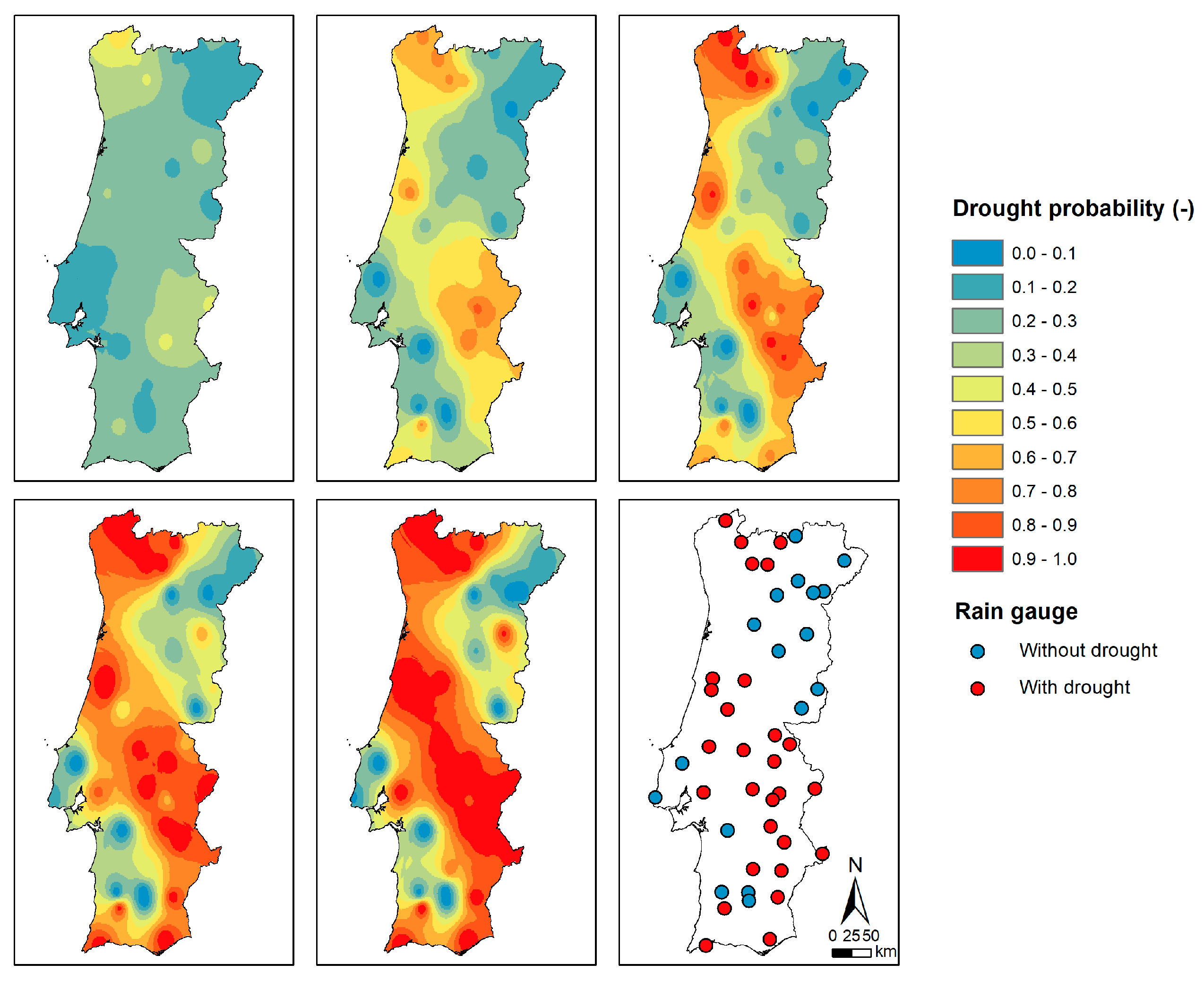
4.3. Drought Risk Monitoring

After the bivariate model has been set up for each rain gauge, the CDPMS was applied to estimate the drought probability, i.e., the temporal evolution of the conditional probability of drought occurrence as new precipitation records are progressively acquired (Equation (2)).
Figure 5 shows the spatial distribution of the moderated drought probability thus achieved for the rainy season of October 2012 to February 2013, chosen as an example. The probability surfaces were obtained by averaging the results at the 45 rain gauges according to the inverse distance weighting (IDW) method with exponent 2.
It is possible to see that, for n = 1 (that is, by the end of October), two regions presented a higher probability of drought occurrence: northwest and southeast regions. For n = 3 (end of December), the probability of drought in those regions increased and even expanded into some of the central areas. As the precipitation in the following months is progressively known, only a few regions of the country have a drought risk smaller than 50%. This could justify issuing an alert regarding a possible drought at the end of March—with caution in December (n = 3), for sure in January (n = 4) and definitely in February (n = 5). Such an early warning could raise the awareness of water resources managers and of civil protection authorities, urging the implementation of some anticipatory measures aiming at mitigating the consequences of a possible scenario of drought and water scarcity.
The last map of Figure 5 shows what happened by the end of March. The almost perfect match between the areas where the drought probability progressively increased with n (areas shaded from blue to orange and red) and those that in fact experienced drought by the end of March (red circles) clearly indicates the ability of the model to identify areas of increasing drought probability.

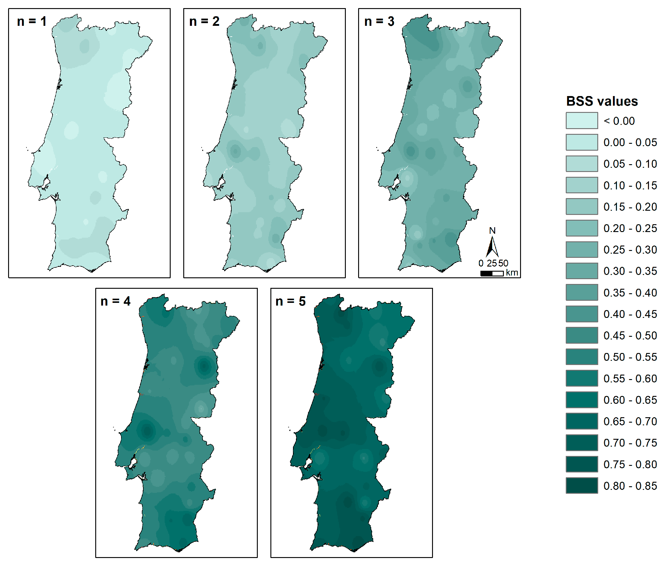
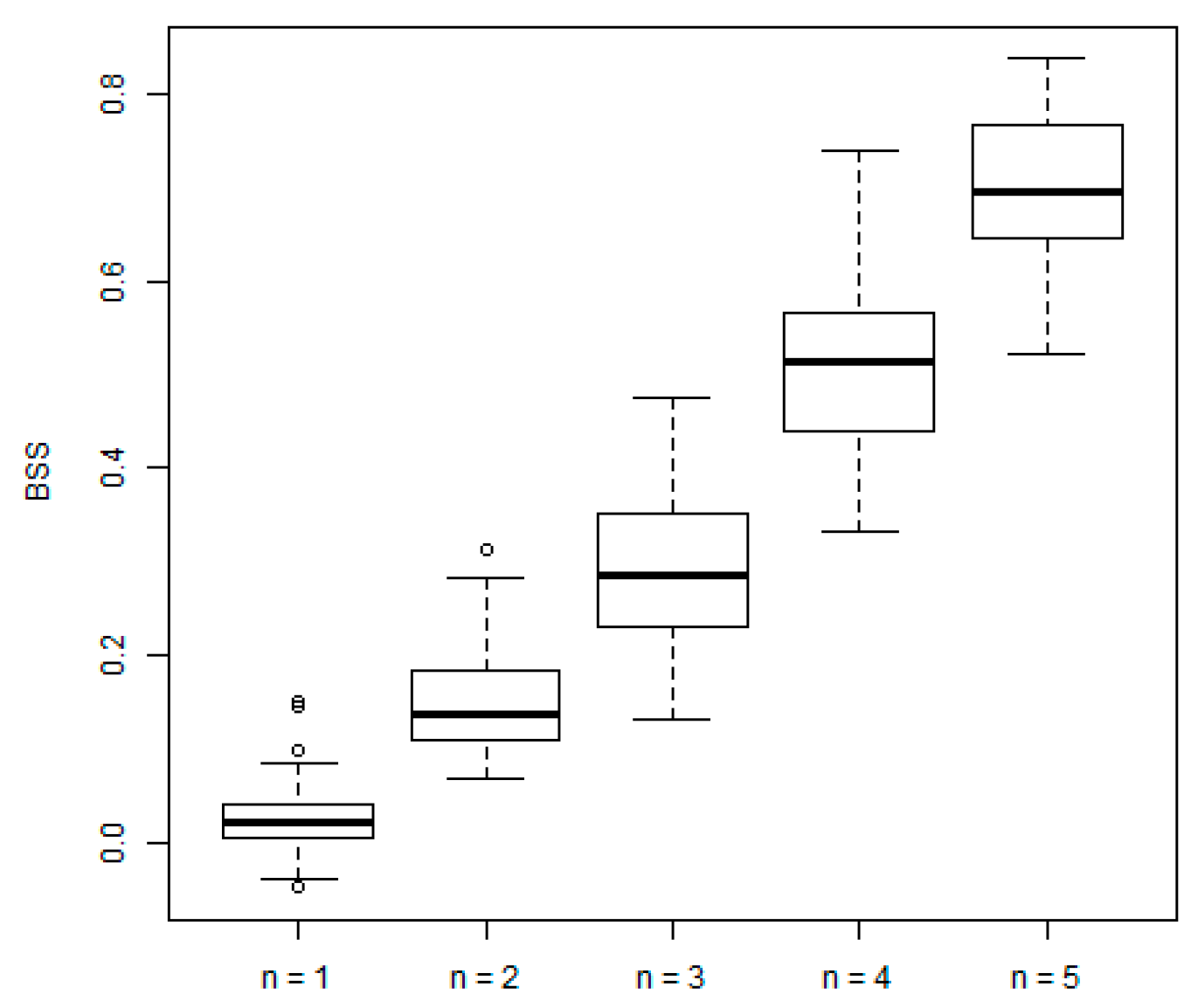
4.4. CDPMS Performance Assessment

The performance of the CDPMS was assessed based on the BSS computed for each one of the 45 rain gauges and values of n, according to the LOOCV methodology (Section 2.2).
The results achieved for predicted moderate droughts are presented in Table 5. The values closer to 1 indicate better model performance, and the negative values indicate that the reference forecast outperformed the CDPMS. The ability of the CDPMS to predict the drought probability increases as the number of months, n, with known precipitation increases: for n = 1 the average performance for the complete set of rain gauges is 0.03 while for n = 5 is 0.70.
The rain gauges where CDPMS had a better performance for n = 1 were RG01, RG06, RG33, RG38, RG41, RG42, and RG43 indicating a higher correlation between the precipitation in October and from October to March (BBS ≥ 0.07). Only for n = 1 and for seven rain gauges (RG02, RG09, RG13, RG19, RG26, RG30, and RG37) did the CDPMS perform worse than the reference forecast (BBS < 0). This means that for these rain gauges the knowledge of the precipitation in October does not allow accurate forecasts of the probability of having or not having drought by the end of March. However, the CDPMS performance increases every month, indicating sustained improvement in the monitoring capabilities as new precipitation data is being collected and provided to the model.
Figure 6 shows the spatial distribution and the evolution of the BSS values for moderate droughts as a function of n, allowing to identify the areas where the CDPMS has better monitoring capabilities (higher values of BSS). The spatial interpolation technique used was also the inverse distance weighting (IDW) with exponent 2.
In order to further analyze the variance of the CDPMS performance, box plots were drawn based on the values of BSS for all rain gauges (Figure 7). The whiskers have a maximum length of 1.5 × IQR (interquartile range), and the values outside the whiskers are outliers.
Figure 7 shows that the variance of the performance measure, BSS, increases in the last two months (n = 4 and n = 5) indicating that, in some rain gauges, a high probability may not result in a drought event as there is still precipitation to fall. The opposite is also true, low risk does not mean drought cannot happen, because the above threshold precipitation tendency presented in the initial months of the rainy season may not be enough to counterbalance the deficits during the last months. However, both specific cases are less likely to occur.
Drought occurrence in mainland Portugal is associated with a substantial interannual and decadal variability, strongly linked to precipitation shortage during the rainy season [38,39]. The dynamic interactions among weather types associated with mainland Portugal due to its location between the Atlantic Ocean and the Mediterranean Sea, strong orographic influence and small size contribute to explain high spatial variability and relative disconnection from general circulation [39,40,41,42]. The complex interactions between different weather types during the rainy season, also as a result of the different geographic conditions, might explain the variability between the model performances.
Overall, due to copula’s high flexibility, a great variety of copula families can be chosen to model the temporal dependence structure of the precipitation in each specific rain gauge, and, by this way, to represent its spatial variability.
The increasing performance of the CDPMS over time means that it consistently learns with the addition of the precipitation in the following months. It also consistently outperforms the reference forecasts, indicating that it can be a valuable source for assessing drought probability.
The application of the LOOCV excluded any bias in the performance verification by not choosing specific years that could best fit the expected performance, such as very dry or very wet years. Therefore, the CDPMS proved to be a valuable tool for drought probability monitoring. However, its application to Mainland Portugal to monitor under real-time conditions the probability of drought by the end of the rainy season requires a continuous updating of the precipitation records at the rain gauges of Figure 2, which may not be an easy task. Alternatively, the CDPMS can be applied to a specific site, as exemplified in the next item.

5. CDRMS Applied to a Single Site

This item refers to the CDPMS development and application to a single site in Mainland Portugal aiming at exemplifying how the system can be operated as a drought monitoring, but also forecasting tool. For this purpose, the rainy season of the hydrological year of 2017/2018 (October 2017 to March 2018) at the rain gauge of Santa Marta da Montanha (RG07) was selected. It was assumed that the precipitation was progressively recorded and provided to the model until February 2018 aiming at estimating the drought probability by the end of the rainy season. As already said, such knowledge is extremely important to develop anticipatory actions and to mitigate impacts related to water scarcity.

5.1. CDRMS Development for Santa Marta da Montanha

The dependence structure for each coupled ( R N , R n ) precipitation series in RG07 rain gauge was modeled by the Archimedean (Frank) and Meta-Elliptical copulas (Gaussian and t Student). Table 6 presents the bivariate models selected for each n, from October (n = 1) to February (n = 5). The parameters θ (for the Archimedean copulas) and ρ and v (for the Meta-Elliptical copulas) were estimated using MPL, and the copula families were selected based on the AIC, as described in Section 2.1.2. The Kendall’s Tau was applied to verify the non-linear dependence between R N and R n modeled by the copulas. A hypothesis test was applied to determine whether R N and R n presented a relevant dependence structure, a small p-value provides strong evidence against the null hypothesis that they are independent, for the 95% confidence level.
The values of the empirical Kendall Tau correlation coefficient presented in Table 6 indicate that as the precipitation in the rainy season is progressively recorded and introduced in the model, the dependence between R N and R n becomes stronger. In fact, for n = 1 the precipitation in October explains only 19% of the precipitation of the rainy season, while for n = 2 it explains 40%, and for n = 5, 83%. The small differences between model and empirical Kendall’s Tau values show that the dependence between R N and, R n was properly modeled by the copulas.
The bivariate model adopted for each coupled ( R N , R n ) series in Santa Marta da Montanha rain gauge is presented in Figure 8. The axes in the figure were graduated in terms of the standard normal deviates that correspond to the non-exceedance probability given by the marginal distributions. The figure shows that as n increases the copulas become narrower due to stronger correlations between R N and R n .

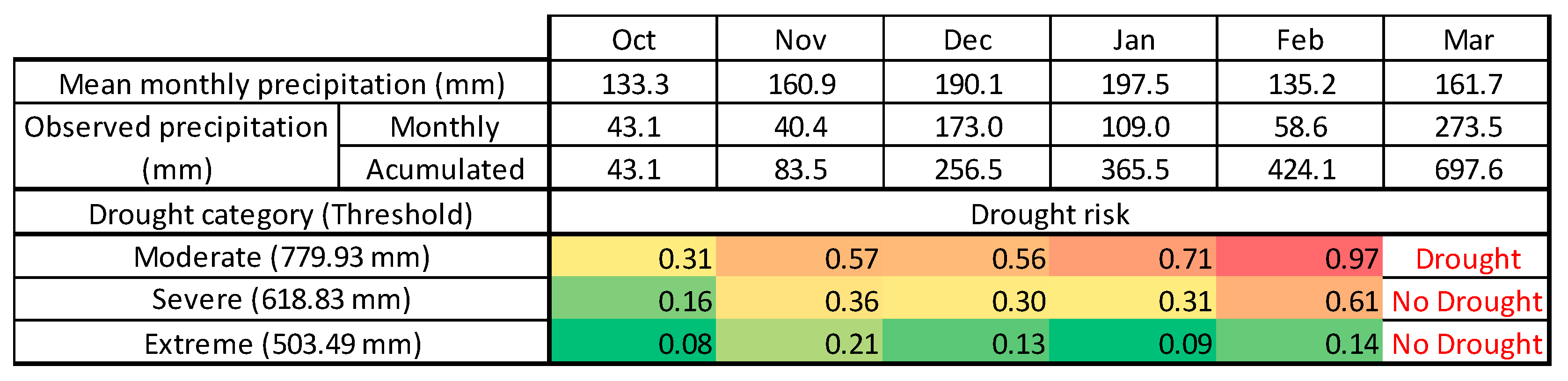
5.2. CDRMS Application—Drought Risk Monitoring

After the bivariate model has been established, the CDPMS was applied to monitor the drought probability in Santa Marta da Montanha rain gauge during the rainy season of 2017/2018. The results obtained are exemplified in the table of Figure 9 for the three categories of droughts, moderate, severe, and extreme droughts. The figure includes the precipitation thresholds, R N * , for the different droughts categories, the precipitation that fell along the season (monthly and cumulative precipitations) and the historical average monthly precipitations.
From October 2017 to March 2018, the total precipitation was 697.6 mm, i.e., below the threshold for moderate drought and above the thresholds for the other drought categories, meaning that a moderate drought event really occurred by the end of March.
In what concerns the moderate droughts, the CDPMS proved to the able to detect the increasing probability of drought: 31% (October 2017), 57% (November 2017), 56% (December 2017), 71% (January 2018), and 97% (February 2018) which could justify issuing a drought alert, at least in January and for sure in February. Despite the considerable above-the-average precipitation that occurred in March, there was a moderate drought, confirming the prediction of CDPMS.
The CDPMS also identified an increased risk of severe drought by the end of March, though with much smaller probability, only 31% in January and 61% in February. However, there was not a severe drought event, which suggests a poorer performance of the CDPMS. This circumstance can be explained by the anomalous and unforeseeable precipitation that took place in March that dampened the expectations of a severe drought.
The last row of the table of Figure 9 indicates very small probabilities of having an extreme drought by the end of March, which was confirmed.
This example shows the capability of CDPMS in detecting moderate droughts. However, the model was not able to distinguish the intensity of the event, once severe and extreme droughts are very sensitive to an individual precipitation event. Precipitation thresholds for the droughts with higher intensity are lower and can be easily exceeded by a few millimeters of precipitation.

6. Discussion and Conclusion

Drought is a harsh natural disaster with onsets difficult to perceive. Therefore, it is relevant and challenging to develop a trustful tool able to recognize its occurrences and to initiate actions aiming at mitigating its impacts. This study developed such a tool, based on copulas applied to the continuous monitoring of the drought probability, using only precipitation data, the CDPMS.
Such a model uses a kind of stepwise procedure applied to each specific location where the drought probability evaluation is required. It starts with the computation of drought-triggering precipitation thresholds, which enable assigning precipitations to the drought categories given by the SPI [23]. The next step refers to the setting up of the copula-based bivariate model that, by using historical monthly precipitation data, “couples” the seasonal precipitation of the rainy season ( R N ) with the precipitation until the last but one month of such season ( R n ), according to the dependence structure between R N and R n .
The last step relates to the application of the CDPMS under current conditions to monitor the drought probability during the rainy season aiming to answer the following question: will there be a drought by the end of the rainy season? Once the precipitation in each month of the current rainy season is progressively known and incorporated into the CDPMS, the model returns the drought probability, that is, the probability of the precipitation being smaller than the one required to avoid drought conditions by the end of the season. Based on that probability, drought warnings can be issued and anticipatory drought mitigation and adaptation measures implemented. The application based on a single rain gauge was exemplified for the rainy season from October 2017 to March 2018.
The CDPMS can also be applied to monitor the evolution of the drought probability during the rainy season in a region, instead of a single site, based on the continuous updating of the precipitation deficits or surplus in the region. Such an innovative application was demonstrated by the application of the CDPMS to Mainland Portugal to monitor the drought probability during the rainy season from October 2012 to March 2013, based on 100-year of precipitation data at 45 rain gauges evenly distributed over the country. The application demonstrated that the CDPMS is able to anticipate the regions that later experienced, in fact, drought conditions.
The study showed that the continuous drought probability monitoring system has the ability to detect drought events simply based on precipitation data. However, it has lower confidence in distinguishing among the drought intensities, probably because the differences among precipitation thresholds for the different intensities are too small and can be easily exceeded by also small, but unforeseeable, amounts of precipitation during the rainy season. The dynamic interactions among weather types associated with Mainland Portugal due to its location between the Atlantic Ocean and the Mediterranean Sea, the strong orographic influence in the precipitation spatial and temporal patterns and its small area may result in the CDPMS performing better in some regions than in others.
Notwithstanding, the CDPMS can help decision-makers to anticipate actions and strategies to decrease potential negative impacts, based on the assignment of a quantitative measure (the probability) to the imminence of a drought event. It also contributes to a systematic warning for water managers and civil protection authorities, allowing them to gradually adjust the public awareness as the threat of a possible drought event becomes more reliable.
The marked seasonality of the rainfall regime in Mainland Portugal makes the precipitation shortages during the rainy season a fundamental trigger of droughts, which explains the good performance of CDPMS despite only based on precipitation data. However, previous studies suggest that, due to the location of the country, the addition of other variables linked to climate, such as teleconnection indexes (North Atlantic Oscillation and sea surface temperature), may improve the drought forecasting capabilities [43,44]. In addition, other climatic and hydrological variables such as temperature and runoff could also be incorporated into the model. Further studies could also try to implement a time-varying copula model for bivariate modeling precipitation ( R N and R n ) designed to address the nonstationary behavior of some of the hydrological variables that is expected to result from climate change [45].

Author Contributions

Conceptualization, methodology, validation, formal analysis, investigation, writing—original draft preparation: J.D.P.F., M.M.P., and T.M.d.C.S.; software, J.D.P.F.; writing—review and editing, supervision: M.M.P., T.M.d.C.S., and F.d.A.S.F.

Funding

Except for the second author, the resaerch was partially supported by grants from the Coordenação de Aperfeiçoamento de Pessoal de Nível Superior—Brasil (CAPES), Conselho Nacional de Desenvolvimento Científico e Tecnológico—Brasil (CNPq), and Fundação Cearense de Apoio ao Desenvolvimento Científico e Tecnológico (FUNCAP)—Finance Code 001.

Conflicts of Interest

The authors declare no conflict of interest.

References

  1. Wilhite, D.A.; Glantz, M.H. Understanding: The Drought Phenomenon: The Role of Definitions. Water Int. 1985, 10, 111–120. [Google Scholar] [CrossRef]
  2. Keyantash, J.; Dracup, J.A. The quantification of drought: An evaluation of drought indices. Bull. Am. Meteorol. Soc. 2002, 83, 1167–1180. [Google Scholar] [CrossRef]
  3. Mishra, A.K.; Singh, V.P. A review of drought concepts. J. Hydrol. 2010, 391, 202–216. [Google Scholar] [CrossRef]
  4. European Commision. Report on the Review of the European Water Scarcity and Droughts Policy; European Commision: Brussels, Belgium, 2012. [Google Scholar]
  5. Heim, R.R. A review of twentieth-century drought indices used in the United States. Bull. Am. Meteorol. Soc. 2002, 83, 1149–1165. [Google Scholar] [CrossRef]
  6. Mckee, T.B.; Doesken, N.J.; Kleist, J. The relationship of drought frequency and duration to time scales. In Proceedings of the 8th Conference on Applied Climatology, Anaheim, CA, USA, 17–22 January 1993; pp. 179–184. [Google Scholar]
  7. Genest, C.; Favre, A.-C. Everything You always wanted to know about copula modeling but were afraid to ask. J. Hydrol. Eng. 2007, 12, 347–368. [Google Scholar] [CrossRef]
  8. Singh, V.P.; Zhang, L. IDF Curves Using the Frank Archimedean Copula. J. Hydrol. Eng. 2007, 12, 651–662. [Google Scholar] [CrossRef]
  9. Chen, L.; Singh, V.P.; Guo, S.; Mishra, A.K.; Guo, J. Drought analysis using copulas. J. Hydrol. Eng. 2013, 18, 797–808. [Google Scholar] [CrossRef]
  10. Lazoglou, G.; Anagnostopoulou, C. Joint distribution of temperature and precipitation in the Mediterranean, using the Copula method. Theor. Appl. Climatol. 2019, 135, 1399–1411. [Google Scholar] [CrossRef]
  11. Hao, Z.; Singh, V.P. Review of dependence modeling in hydrology and water resources. Prog. Phys. Geogr. 2016, 40, 549–578. [Google Scholar] [CrossRef]
  12. Aas, K.; Czado, C.; Frigessi, A. Pair-copula constructions of multiple dependence Projektpartner Pair-copula constructions of multiple dependence. Insur. Math. Econ. 2009, 44, 182–198. [Google Scholar] [CrossRef]
  13. Shiau, J.T. Fitting drought duration and severity with two-dimensional copulas. Water Resour. Manag. 2006, 20, 795–815. [Google Scholar] [CrossRef]
  14. Xu, K.; Yang, D.; Xu, X.; Lei, H. Copula based drought frequency analysis considering the spatio-temporal variability in Southwest China. J. Hydrol. 2015, 527, 630–640. [Google Scholar] [CrossRef]
  15. Chen, X.; Li, F.; Li, J.; Feng, P. Three-dimensional identification of hydrological drought and multivariate drought risk probability assessment in the Luanhe River basin, China. Theor. Appl. Climatol. 2019. [Google Scholar] [CrossRef]
  16. Ayantobo, O.O.; Li, Y.; Song, S.; Javed, T.; Yao, N. Probabilistic modelling of drought events in China via 2-dimensional joint copula. J. Hydrol. 2018, 559, 373–391. [Google Scholar] [CrossRef]
  17. Montaseri, M.; Amirataee, B.; Rezaie, H. New approach in bivariate drought duration and severity analysis. J. Hydrol. 2018, 559, 166–181. [Google Scholar] [CrossRef]
  18. Kao, S.C.; Govindaraju, R.S. A copula-based joint deficit index for droughts. J Hydrol. 2010, 380, 121–134. [Google Scholar] [CrossRef]
  19. Chang, J.; Li, Y.; Wang, Y.; Yuan, M. Copula-based drought risk assessment combined with an integrated index in the Wei River Basin, China. J Hydrol. 2016, 540, 824–834. [Google Scholar] [CrossRef]
  20. Liu, Y.; Zhu, Y.; Ren, L.; Yong, B.; Singh, V.P.; Yuan, F.; Jiang, S.; Yang, X. On the mechanisms of two composite methods for construction of multivariate drought indices. Sci. Total Environ. 2019, 647, 981–991. [Google Scholar] [CrossRef]
  21. Tosunoglu, F.; Can, I. Application of copulas for regional bivariate frequency analysis of meteorological droughts in Turkey. Nat. Hazards 2016. [Google Scholar] [CrossRef]
  22. Shin, J.Y.; Chen, S.; Lee, J.-H.; Kim, T.-W. Investigation of drought propagation in South Korea using drought index and conditional probability. Terr. Atmos. Ocean. Sci. 2018, 29, 231–241. [Google Scholar] [CrossRef] [Green Version]
  23. Portela, M.M.; dos Santos, J.F.F.; Naghettini, M.; Matos, J.P.; Silva, A.T. Superfícies de limiares de precipitação para identificação de secas em Portugal continental: Uma aplicação complementar do Índice de Precipitação Padronizada, SPI. Rev. Recur. Hídricos. 2012, 33, 5–23. [Google Scholar] [CrossRef]
  24. Dos Santos, J.F.F.; Portela, M.M.; Naghettini, M.; Matos, J.P.; Silva, A.T. Precipitation thresholds for drought recognition: A complementary use of the standardized precipitation index, SPI. River Basin Manag. 2013. [Google Scholar] [CrossRef]
  25. Dos Santos, J.F.F. Drought Analysis in Mainland Portugal: Spatial Distribution, Frequency and Hindcasting. Ph.D. Thesis, Instituto Superior Técnico, Lisbon, Portugal, 2012. [Google Scholar]
  26. Agnew, C. Using the SPI to identify drought. Drought Netw. News 2000, 12, 5–12. [Google Scholar]
  27. Nelsen, R.B. An Introduction to Copulas, 2nd ed.; Springer: New York, NY, USA, 2006; pp. 1–656. [Google Scholar]
  28. Ayantobo, O.O.; Li, Y.; Song, S. Multivariate drought frequency analysis using four-variate symmetric and asymmetric archimedean copula functions. Water Resour. Manag. 2019, 33, 103–127. [Google Scholar] [CrossRef]
  29. Zhang, Q.; Xiao, M.; Singh, V.P.; Chen, X. Copula-based risk evaluation of hydrological droughts in the East River basin, China. Stoch. Environ. Res. Risk Assess. 2013. [Google Scholar] [CrossRef]
  30. Sharifi, E.; Saghafian, B.; Steinacker, R. Copula-based stochastic uncertainty analysis of satellite precipitation products. J Hydrol. 2019, 570, 739–754. [Google Scholar] [CrossRef]
  31. Joe, H. Multivariate Models and Dependence Concepts; Chapman & Hall: London, UK, 1997. [Google Scholar]
  32. Genest, C.; Ghoudi, K.; Rivest, L.P. A semiparametric estimation procedure of dependence parameters in multivariate families of distributions. Biometrika 1995, 82, 543–552. [Google Scholar] [CrossRef]
  33. Brechmann, E.C.; Schepsmeier, U. Modeling Dependence with C- and D-Vine Copulas: The R Package CDVine. J. Stat. Softw. 2013, 52. [Google Scholar] [CrossRef]
  34. Wilks, D.S. Statistical Methods in the Atmospheric Sciences; Academic Press: Cambridge, MA, USA, 2011; pp. 2–676. [Google Scholar]
  35. Klein, B.; Meissner, D.; Kobialka, H.-U.; Reggiani, P. Predictive Uncertainty Estimation of Hydrological Multi-Model Ensembles Using Pair-Copula Construction. Water 2016, 8, 125. [Google Scholar] [CrossRef]
  36. Hao, Z.; Hao, F.; Singh, V.P.; Zhang, X. Statistical prediction of the severity of compound dry-hot events based on El Niño-Southern Oscillation. J. Hydrol. 2019. [Google Scholar] [CrossRef]
  37. Portela, M.M.; Zeleňáková, M.; dos Santos, J.F.F.; Purcz, P.; Silva, A.T.; Hlavatá, H. A comprehensive drought analysis in Slovakia using SPI. Eur Water. 2015, 51, 15–31. [Google Scholar]
  38. Russo, A.C.; Gouveia, C.M.; Trigo, R.M.; Liberato, M.L.R.; DaCamara, C.C. The influence of circulation weather patterns at different spatial scales on drought variability in the Iberian Peninsula. Front. Environ. Sci. 2015, 3, 1–15. [Google Scholar] [CrossRef]
  39. Trigo, R.M.; DaCamara, C.C. Circulation weather types and their influence on the precipitation regime in Portugal. Int. J. Climatol. 2000, 20, 1559–1581. [Google Scholar] [CrossRef]
  40. Trigo, R.M.; Valente, M.A.; Trigo, I.F.; Miranda, P.M.A.; Ramos, A.M.; Paredes, D.; García-Herrera, R. The impact of North Atlantic wind and cyclone trends on European precipitation and significant wave height in the Atlantic. Ann. N Y Acad. Sci. 2008, 1146, 212–234. [Google Scholar] [CrossRef] [PubMed]
  41. Trigo, R.M.; Pozo-Vázquez, D.; Osborn, T.J.; Castro-Díez, Y.; Gámiz-Fortis, S.; Esteban-Parra, M.J. North Atlantic oscillation influence on precipitation, river flow and water resources in the Iberian Peninsula. Int. J. Climatol. 2004, 24, 925–944. [Google Scholar] [CrossRef]
  42. Cortesi, N.; Gonzalez-Hidalgo, J.C.; Trigo, R.M.; Ramos, A.M. Weather types and spatial variability of precipitation in the Iberian Peninsula. Int. J. Climatol. 2014, 34, 2661–2677. [Google Scholar] [CrossRef]
  43. Santos, J.F.; Portela, M.M.; Pulido-Calvo, I. Spring drought prediction based on winter NAO and global SST in Portugal. Hydrol. Process. 2014, 28, 1009–1024. [Google Scholar] [CrossRef]
  44. Del Valle García Valdecasas Ojeda, M.M. Climate-Change Projections in the Iberian Peninsula: A Study on the Hydrological Impacts. Ph.D. Thesis, Universidad de Granada, Granada, Spain, 2018. [Google Scholar]
  45. Silva, A.T. Nonstationarity and Uncertainty of Extreme Hydrological Events. Ph.D. Thesis, Instituto Superior Técnico, Lisbon, Portugal, 2018. [Google Scholar]
Figure 1. Mainland Portugal. Surfaces of precipitation thresholds, R N * , for the 6-month period from October to March (SPI6), from the right to the left, for moderate (−0.84), severe (−1.28), and extreme (−1.65) droughts. Adapted from [23].
Water 11 01925 g001
Figure 2. Development of the CDPMS and evaluation of its performance.
Water 11 01925 g002
Figure 3. Location of the 45 rain gauges used in the study.
Water 11 01925 g003
Figure 4. Distribution (in percentage) of the selected copulas by the 45 rain gauges as a function of the number of initial months of the rainy season.
Water 11 01925 g004
Figure 5. Example of the application of the CDPMS to the continuous monitoring of the likelihood of moderate drought at the end of the six months period from October 2012 to February 2013. Drought probability from the end of October (n = 1) to the end of February (n = 5). The last map identifies the rain gauges that in fact did or did not experience drought by the end of March of 2013.
Water 11 01925 g005
Figure 6. Moderate droughts. BSS values for n = 1 to n = 5. The closer to 1, the better the CDRMS performance.
Water 11 01925 g006
Figure 7. Moderate droughts. BSS values for all the rain gauges as a function of the number of initial months of the rainy season with known precipitation (n).
Water 11 01925 g007
Figure 8. Santa Marta da Montanha (RG07) rain gauge. Bivariate models for each coupled ( R N , R n ) series along the rainy season of 2017/2018, from n = 1 to 5.
Water 11 01925 g008
Figure 9. Santa Marta da Montanha (RG07) rain gauge. Probability of moderate, severe, and extreme drought events along the rainy season of 2017/2018 according to the CDPMS (dashed cells).
Water 11 01925 g009
Table 1. Classes of drought intensity, associated probability, and SPI value according to [26].
Drought ClassProbabilitySPI Value
Moderate Drought0.20Less than −0.84
Severe Drought0.10Less than −1.28
Extreme Drought0.05Less than −1.65
Table 2. Copula candidate family formulation and parameter range.
ClassFamily C ( u 1 , u 2 ) Parameter Range
ArchimedeanGumbel exp { [ ( ln u 1 )   θ + ( ln u 2 )   θ ] 1   θ θ   [ 1 ,   + )
ArchimedeanFrank 1 θ log   ( 1 +   ( e θ   u 1 1 ) ( e θ   u 2 1 ) ( e θ 1 ) ) θ   ( ,   + )
ArchimedeanClayton ( u 1 θ +   u 2 θ 1 ) 1 θ ) θ   ( 0 ,   + )
Meta-EllipticalGaussian ϕ ρ ( ϕ 1 ( u 1 ) ,   ϕ 1 ( u 2 ) ) ρ     ( 1 , 1 )
Meta-Ellipticalt Student T ρ , v ( T v 1 ( u 1 ) ,   T v 1 ( u 2 ) ) ρ     ( 1 , 1 ) ,   v > 2  
Table 3. Name, code, identification (ID), and geographic coordinates (WGS84 system) of the 45 rain gauges of Figure 3.
NameCodeIDLat (°)Long (°)
Merufe01G03UGRG0142.0180−8.3890
Travancas03N01GRG0241.8280−7.3056
Leonte03I03UGRG0341.7650−8.1470
Soutelo (Chaves)03L02UGRG0441.7530−7.5348
Campo de Víboras04R03UGRG0541.5240−6.5580
Cabeceiras de Basto04J06UGRG0641.5127−7.9792
Santa Marta da Montanha04K02GRG0741.5008−7.7460
Folgares06N01CRG0841.3032−7.2828
Carviçais06P02UGRG0941.1790−6.8900
Moncorvo06O04UGRG1041.1650−7.0510
Adorigo07L01URG1141.1460−7.6070
Pindelo dos Milagres09J02URG1240.8060−7.9630
Freixedas09O02URG1340.6880−7.1630
Gouveia11L01UGRG1440.4940−7.5930
Santo Varão12F02CRG1540.1840−8.6020
Góis13I01GRG1640.1568−8.1133
Soure13F01GRG1740.0521−8.6250
Penha Garcia13O01UGRG1840.0420−7.0180
Alvaiázere15G01UGRG1939.8270−8.3810
Ladoeiro14N02UGRG2039.8269−7.2660
Nisa16L03UGRG2139.5160−7.6690
Castelo de Vide17M01GRG2239.4116−7.4525
Pernes17F01UGRG2339.3910−8.6630
Bemposta17I02UGRG2439.3490−8.1410
Alter do Chão18L01UGRG2539.2182−7.6844
Pragança18C01GRG2639.1990−9.0640
Pavia20I01GRG2738.8965−8.0136
Caia (Monte Caldeiras)20O02UGRG2838.8873−7.0898
Santo Estevão20E02UGRG2938.8600−8.7460
Estremoz20L01GRG3038.8416−7.6159
Colares (Sarrazola)21A01CRG3138.8020−9.4570
Évora−Monte21K02UGRG3238.7690−7.7161
São Manços23K01UGRG3338.4605−7.7505
Barragem de Pego do Altar23G01CRG3438.4196−8.3952
Amieira24L01CRG3538.2793−7.5605
Barrancos25P01UGRG3638.1321−7.0013
Santa Vitória26I01UGRG3737.9645−8.0227
Serpa26L01UGRG3837.9426−7.6038
Relíquias27G01GRG3937.7030−8.4825
Castro Verde27I01GRG4037.6976−8.0933
Mértola28L01UGRG4137.6371−7.6619
Rosário (Almodôvar)28I02URG4237.6020−8.0810
Barragem de Mira28G01CRG4337.5101−8.4433
Santa Catarina (Tavira)31K01UGRG4437.1487−7.7847
Valverde31E03CRG4537.0820−8.7180
Table 4. Precipitation thresholds, R N * , (mm) for the six-month period, from October to March, for the different drought intensities.
Rain Gauge IDDrought IntensityRain Gauge IDDrought Intensity
ModerateSevereExtremeModerateSevereExtreme
RG01745.2550.6411.7RG23379.6288.8218.2
RG02429.9351.9297.6RG24307.4226.9165.0
RG031250.0933.9701.4RG25269.9190.0126.2
RG04338.9272.4228.7RG26442.1357.1294.9
RG05252.7212.2189.9RG27245.4181.4132.1
RG06624.0467.6350.5RG28228.6169.4122.5
RG07774.4614.7500.8RG29272.3208.9160.4
RG08250.9197.3158.8RG30281.6208.1151.8
RG09290.0221.5172.2RG31371.7309.3263.1
RG10225.0175.0137.3RG32265.6201.5152.4
RG11280.2223.0182.2RG33238.9178.1130.7
RG12601.4479.3393.2RG34269.6214.9174.6
RG13311.6232.8170.6RG35256.2202.4162.6
RG14517.3419.1345.1RG36260.6204.4160.0
RG15446.4361.0294.2RG37251.9197.7155.9
RG16557.5449.0364.9RG38237.9182.4140.6
RG17415.4320.1246.6RG39311.3242.3191.1
RG18383.7310.8255.6RG40267.9215.7175.7
RG19586.6468.6378.5RG41184.5146.8120.9
RG20288.6234.7194.2RG42284.4223.2176.3
RG21331.5256.7199.4RG43292.3225.8173.2
RG22370.7284.5221.8RG44318.5239.5180.3
RG45289.5229.0182.3
Table 5. Moderate droughts. BSS values for n = 1 to n = 5.
Rain Gauge IDn = 1n = 2n = 3n = 4n = 5Average
RG010.150.270.460.570.690.43
RG02−0.020.100.130.370.550.23
RG030.050.190.470.630.830.44
RG040.040.100.250.440.650.30
RG050.000.180.350.510.650.34
RG060.150.270.440.550.770.44
RG070.060.180.350.520.660.35
RG080.040.110.230.410.560.27
RG09−0.030.250.270.530.620.33
RG100.010.160.220.410.520.27
RG110.020.140.220.530.640.31
RG120.010.130.280.440.590.29
RG13−0.030.140.390.710.790.40
RG140.000.110.230.520.660.30
RG150.020.190.320.440.700.33
RG160.010.110.230.500.730.32
RG170.020.130.310.540.810.36
RG180.000.120.230.440.580.27
RG19−0.020.090.210.500.700.29
RG200.010.070.210.330.650.25
RG210.010.100.290.420.740.31
RG220.000.130.310.470.690.32
RG230.010.310.440.740.830.47
RG240.030.230.380.560.810.40
RG250.020.150.300.570.730.35
RG26−0.050.120.250.600.780.34
RG270.030.170.300.410.670.32
RG280.030.180.290.470.720.34
RG290.020.100.140.410.550.24
RG30−0.040.110.270.400.540.25
RG310.030.070.240.510.730.32
RG320.050.150.250.490.620.31
RG330.080.210.370.480.670.36
RG340.010.130.270.410.680.30
RG350.010.110.320.570.710.34
RG360.040.190.290.540.680.35
RG37−0.010.140.290.570.840.36
RG380.070.240.310.480.570.33
RG390.040.170.150.540.710.32
RG400.030.130.310.610.800.37
RG410.100.280.470.700.810.47
RG420.070.160.420.660.780.42
RG430.080.200.370.540.700.38
RG440.030.080.350.660.820.39
RG450.010.140.190.470.760.32
Average0.030.160.300.510.700.34
Table 6. Santa Marta da Montanha (RG07) rain gauge. Bivariate models for each coupled ( R N , R n ) series, their parameters, Kendall Tau correlation (according to the model and empirical), AIC, and p values.
R n FamilyParametersKendall’s TauAICp-Value
θ   or     ρ v ModelEmpirical
n = 1 Frank1.75-0.190.19−6.16<0.05
n = 2Gaussian 0.60-0.410.40−37.86<0.05
n = 3t Student 0.7630.000.550.53−75.34<0.05
n = 4Gaussian0.91-0.720.72−161.84<0.05
n = 5Gaussian0.96-0.830.83−251.14<0.05

