Comparative Analysis of Building Representations in TELEMAC-2D for Flood Inundation in Idealized Urban Districts


Abstract
1. Introduction
- urban areas are more complex than rural areas owing to more artificial infrastructure;
- receiving precise Digital Elevation Model (DEM) data that records variations in urban micro-topography is difficult;
- related data such as depth and velocity are difficult to observe in fact, and for an entire flow area, data provided via aerial imagery is insufficient.
- to build TELEMAC-2D models and verify their applicability to urban flooding;
- to compare the results of different building representation methods using numerical modeling;
- to analyze the influence of building layouts and mesh resolutions.
2. Methods and Materials
2.1. TELEMAC-2D Model
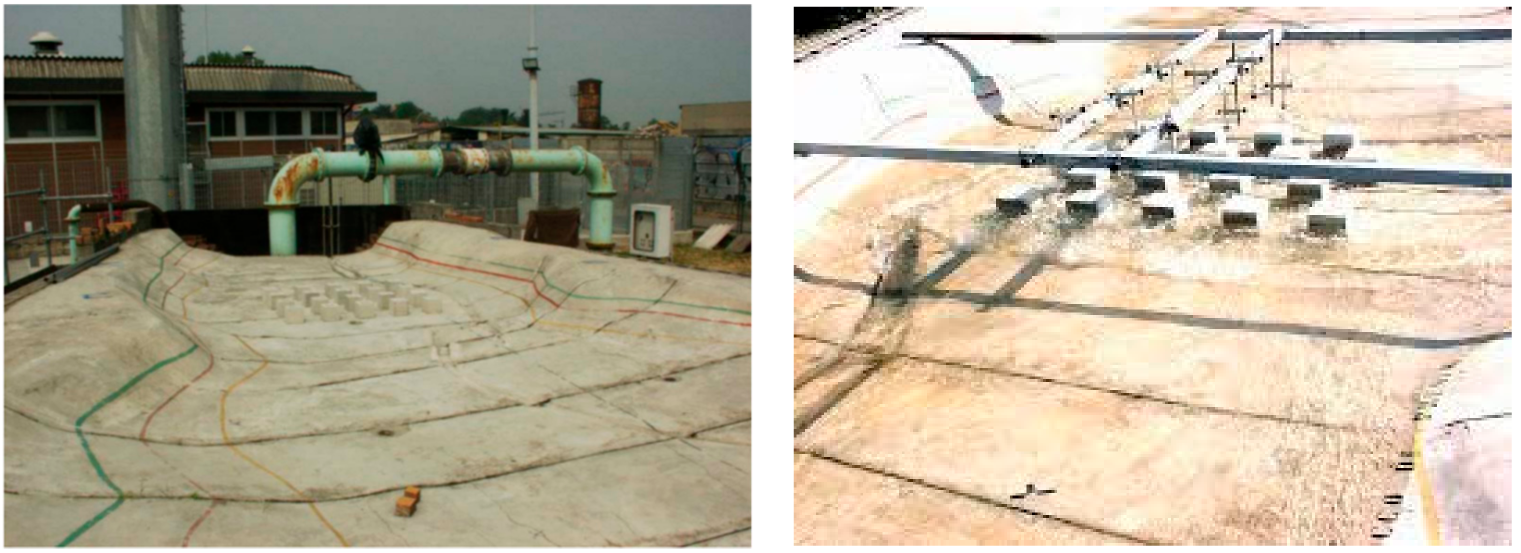
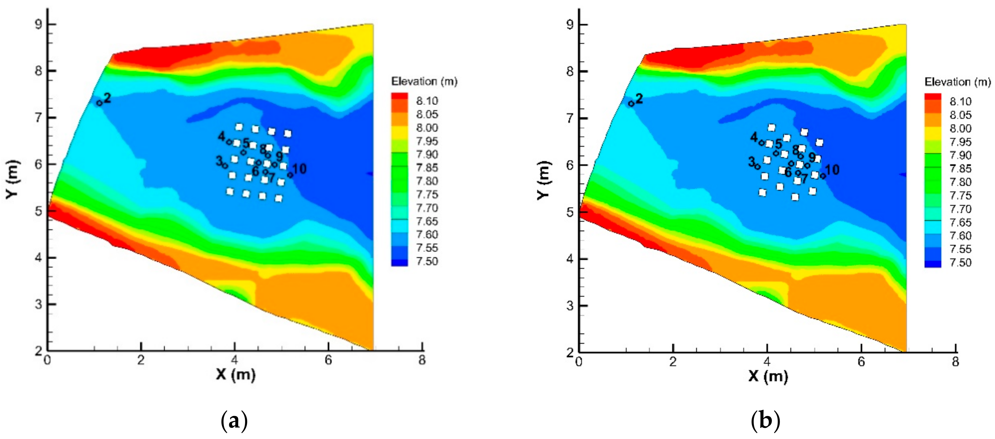
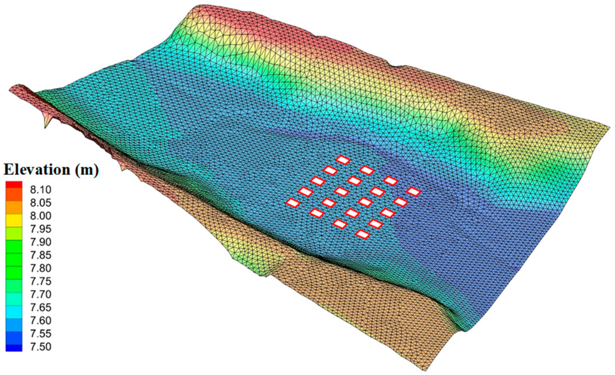
2.2. Toce River Valley Case
2.3. Three Different Building Representations
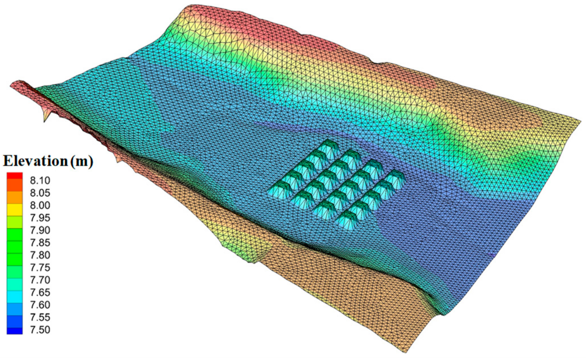
2.3.1. Building–Hole Method
2.3.2. Building–Block Method
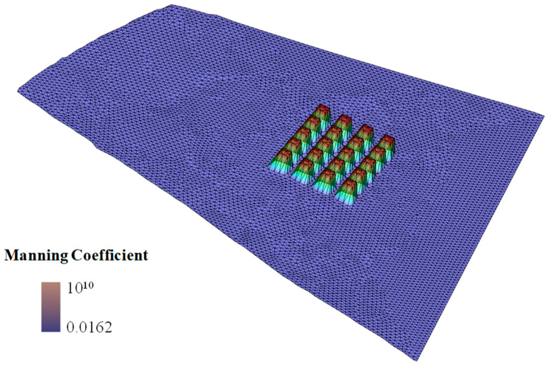
2.3.3. Building–Resistance Method
2.4. Numerical Experiment Setup
3. Results
3.1. Analysis of Different Mesh Resolutions
3.2. Manning Coefficient Sensitivity Analysis
3.3. Analysis of Results for Different Building Representations
4. Discussion
4.1. Model Performance with Different Building Representations, Manning Coefficients, and Mesh Resolutions
4.2. Abnormal Results Analysis
4.3. Further Considerations and Suggestions
5. Conclusions
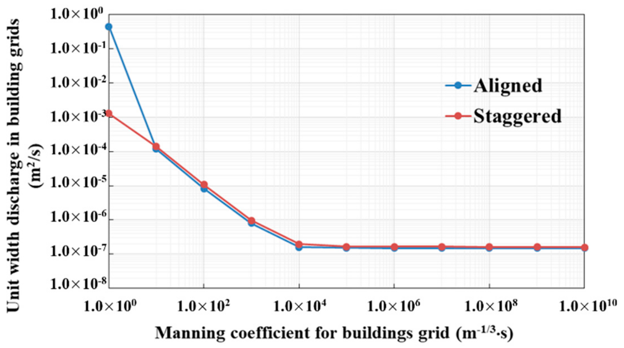
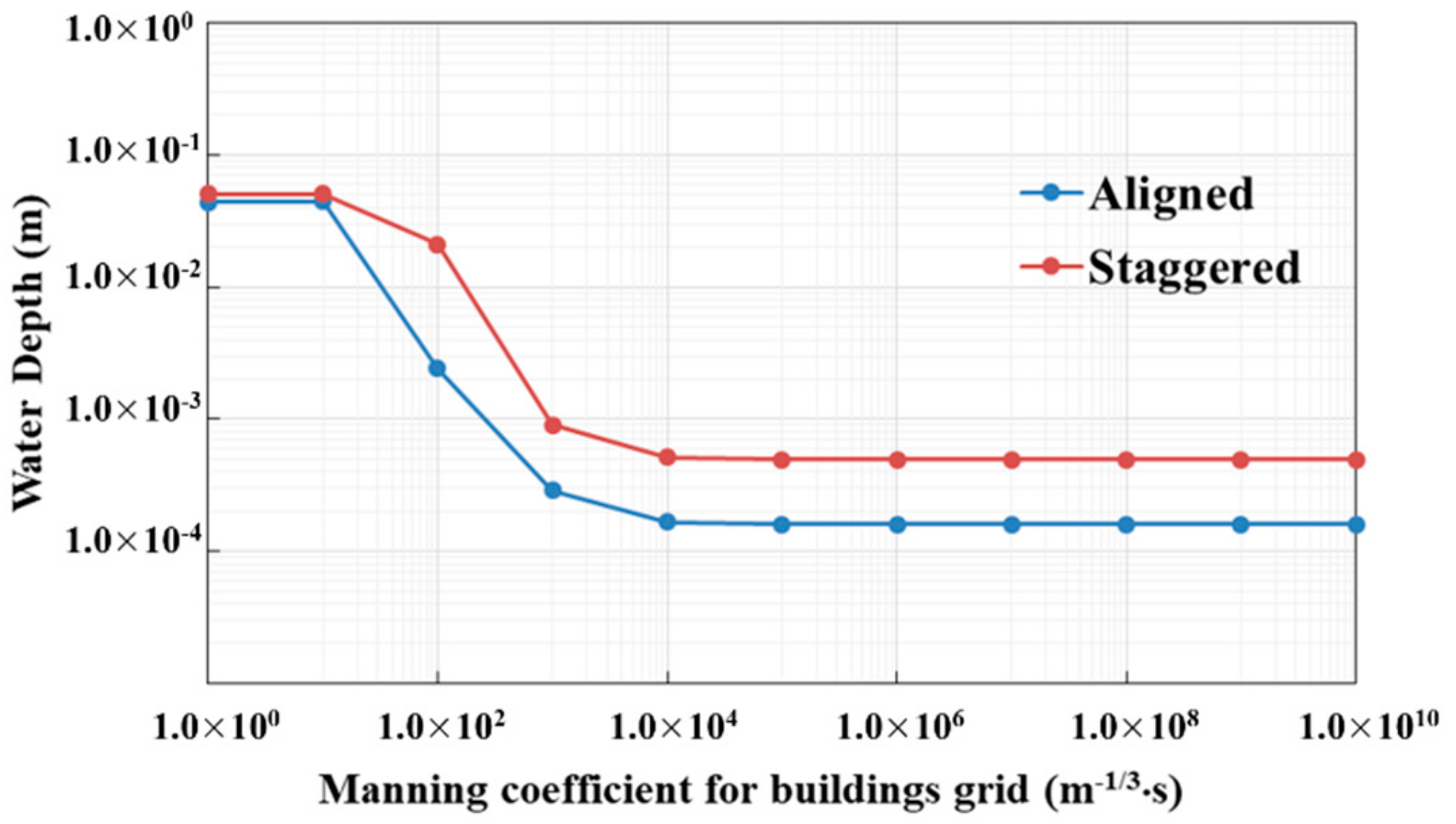
- In the BR method, the Manning coefficient is an important parameter because it represents the amount of flood flow passing through the building grids. Based on sensitivity analysis, the Manning coefficient is not sensitive when it is larger than 104 ; furthermore, the unit-width discharge and water depth in the building grids decreases as the Manning coefficient increases when the Manning coefficient is less than 104 .
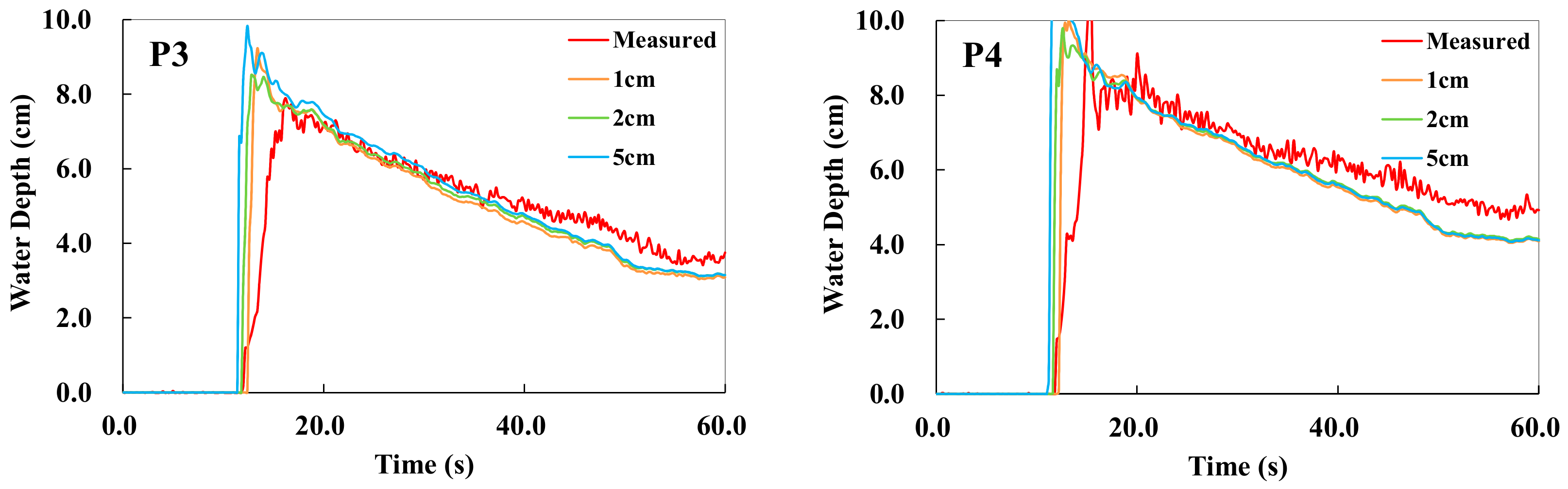
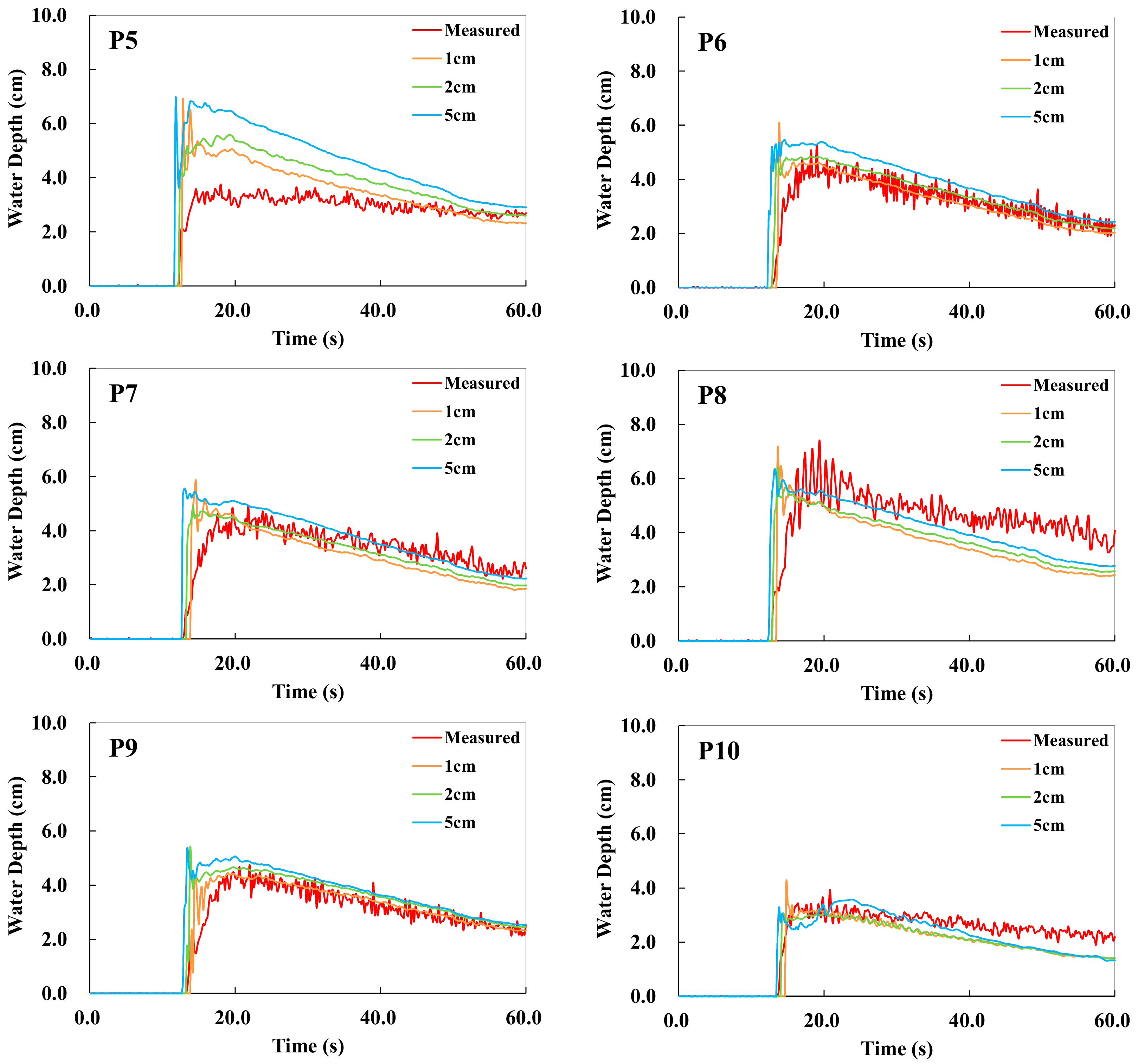
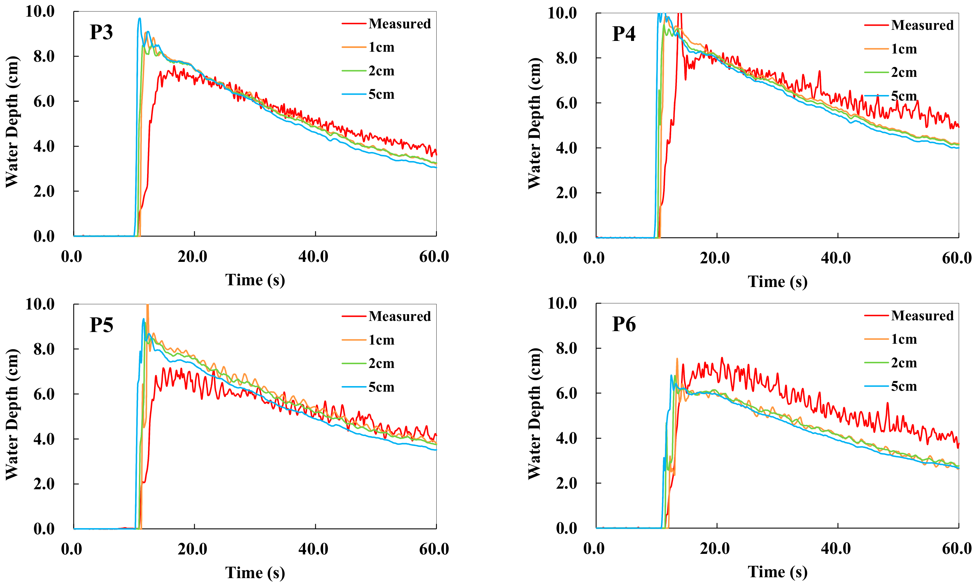
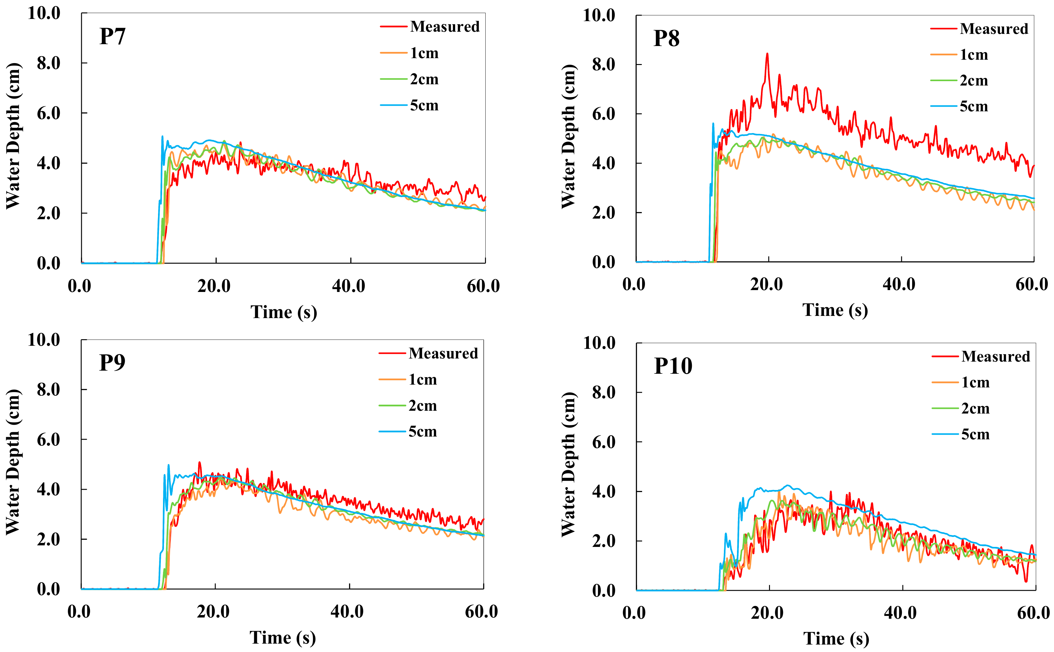
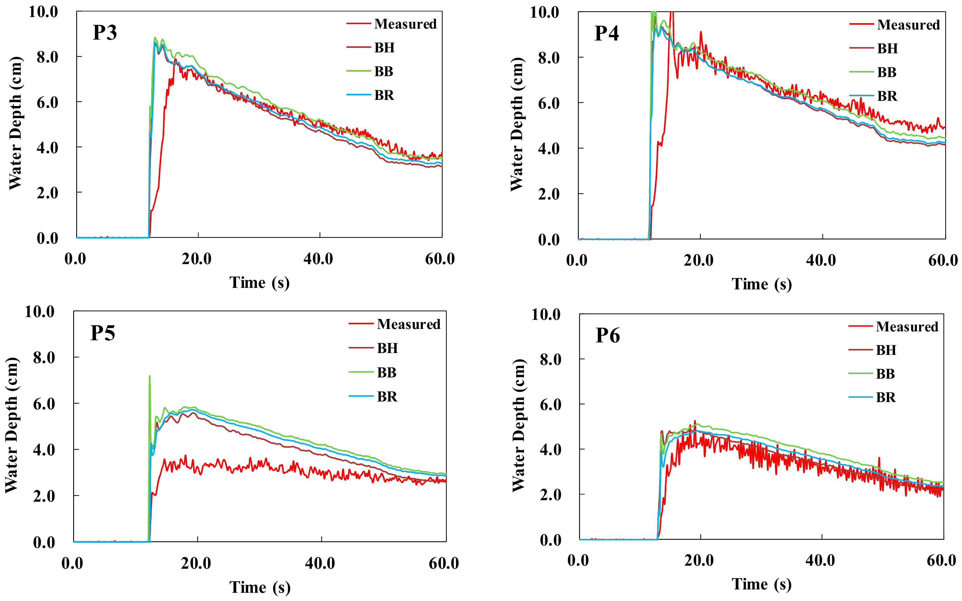
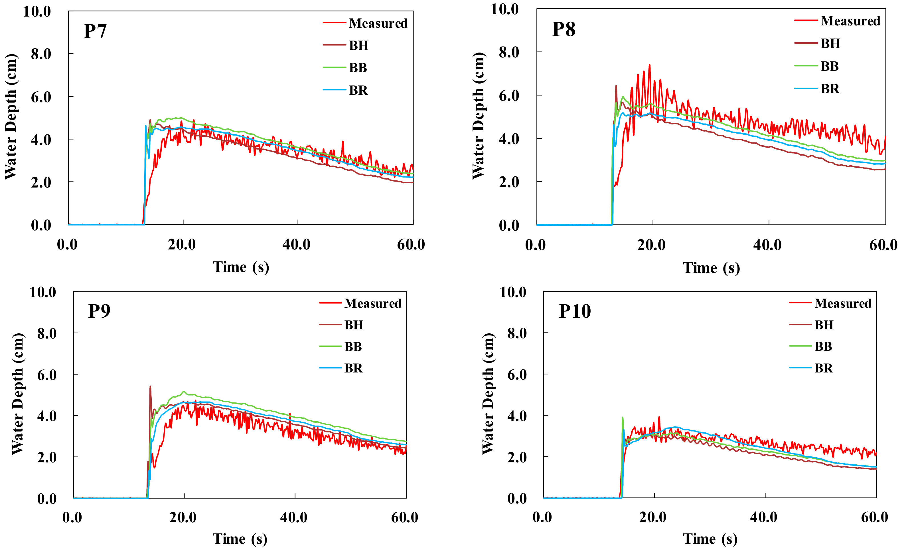
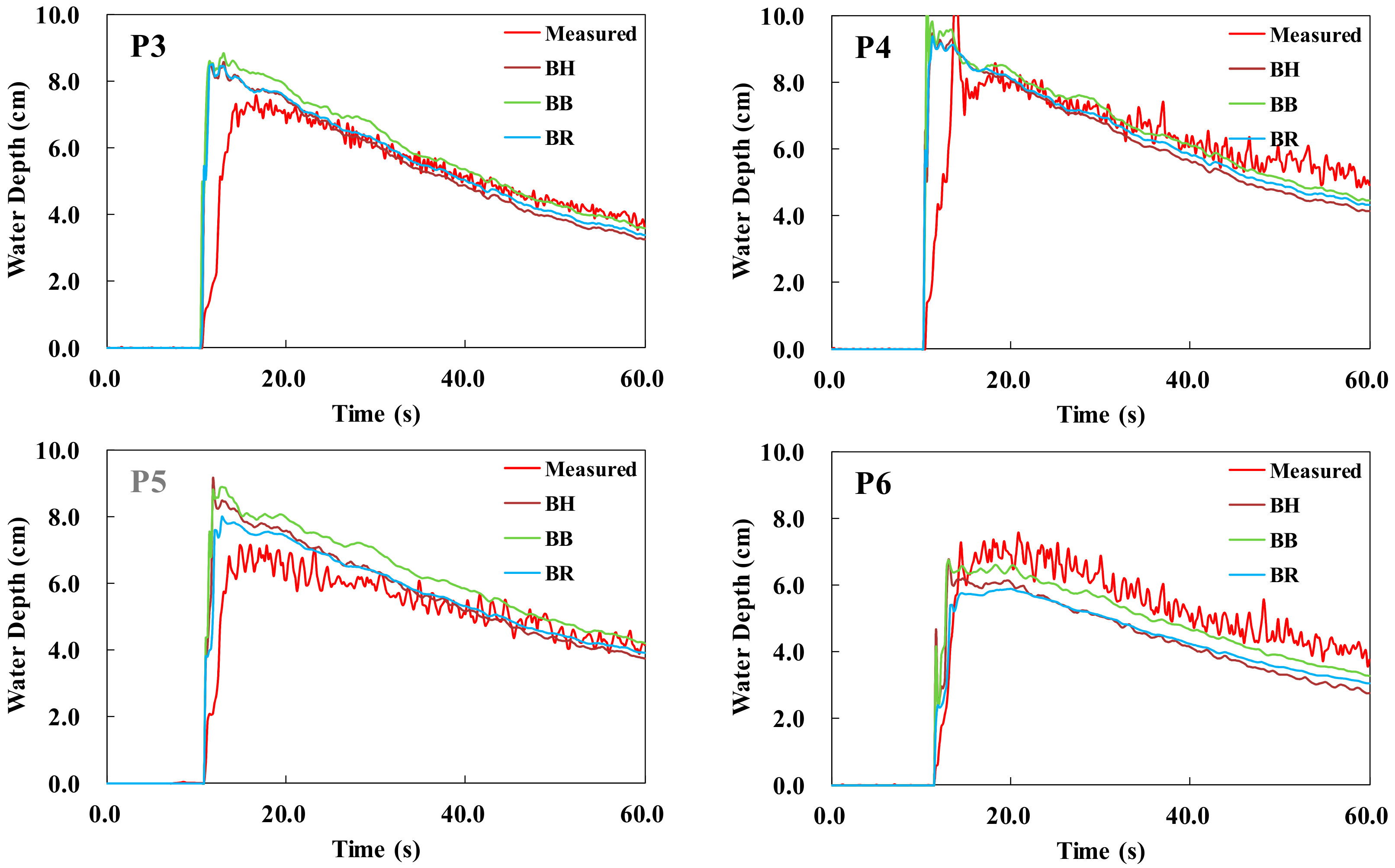
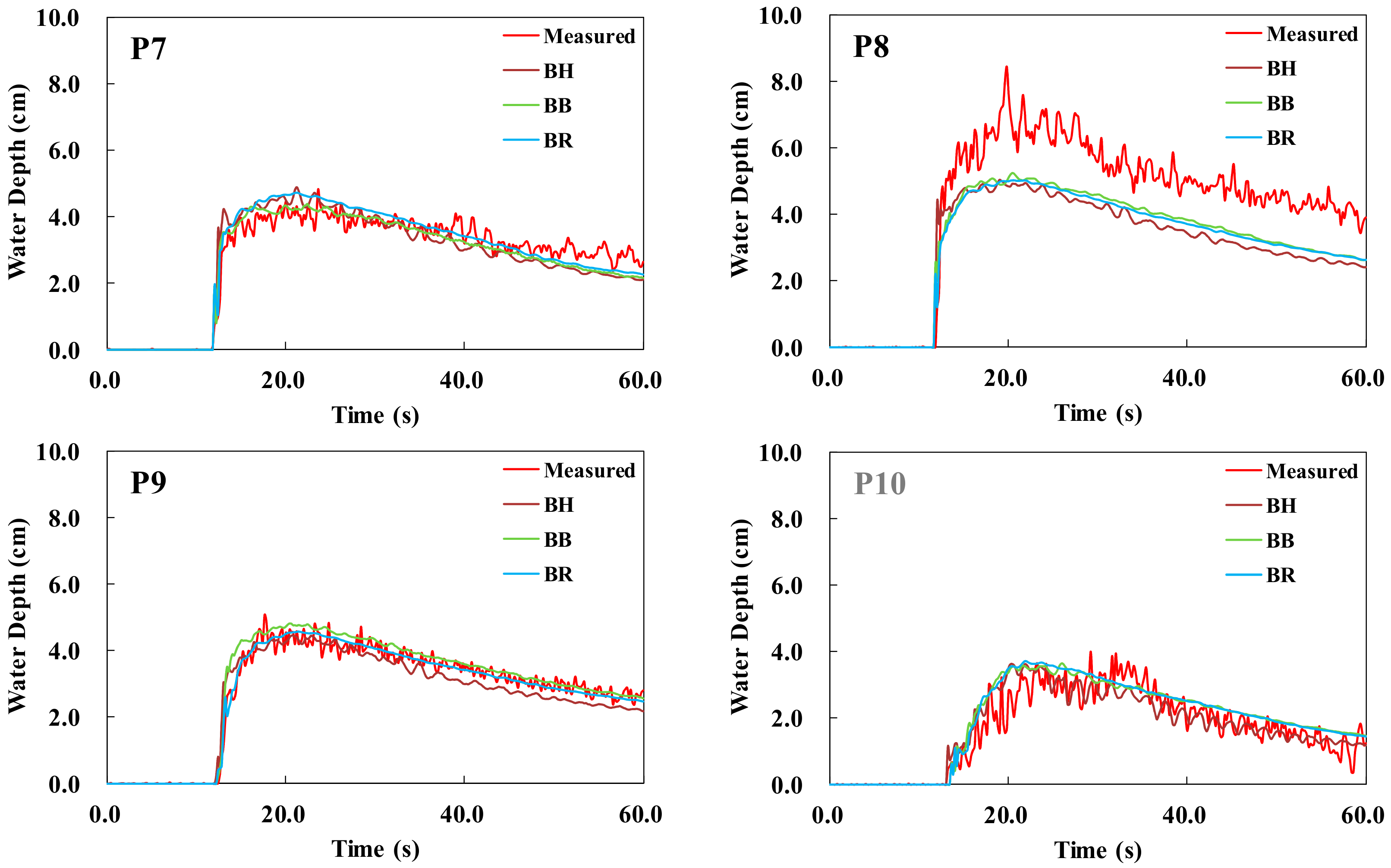
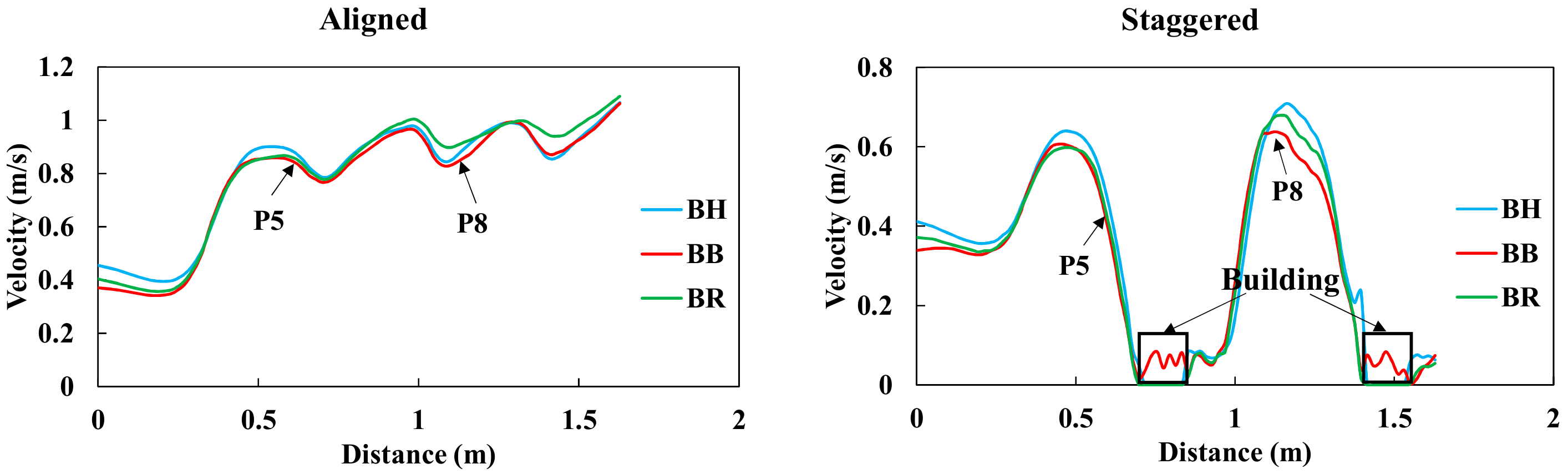
- The TELEMAC-2D model can simulate urban flooding with complex underlying surfaces. The model results obtained herein from the three building representation methods are mostly consistent with measured values. However, some differences exist in the simulation results: e.g., the peak water-level values are slightly greater than the measured values, and the peak time falls ahead of the observed value. Results demonstrate that the TELEMAC-2D model is largely applicable to the simulation of urban flooding. As there are obvious differences at some locations (e.g., at gauges P5 and P8), the modeling methods need to be further optimized and model parameters need to be reasonably adjusted based on actual complex situations.
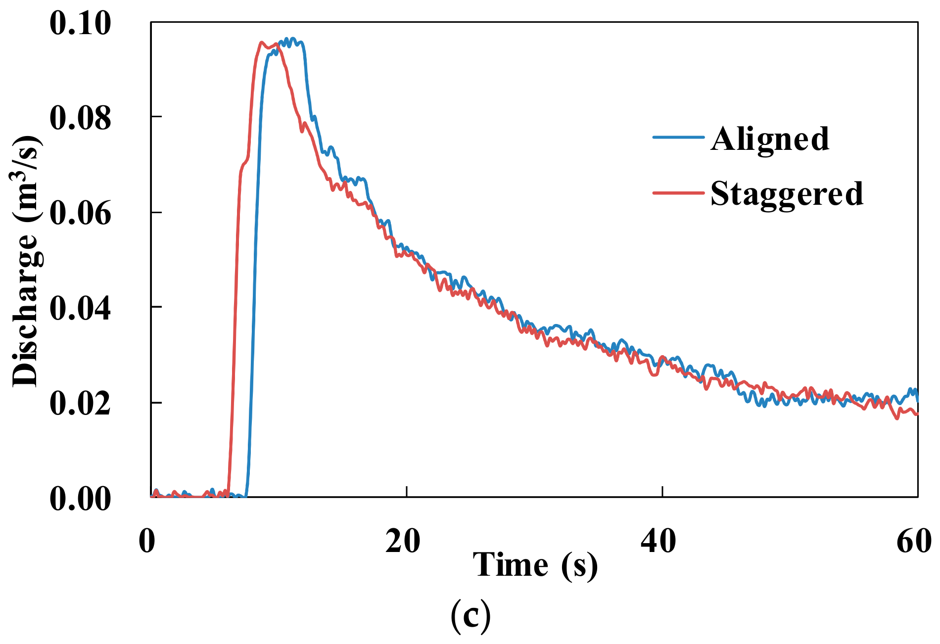
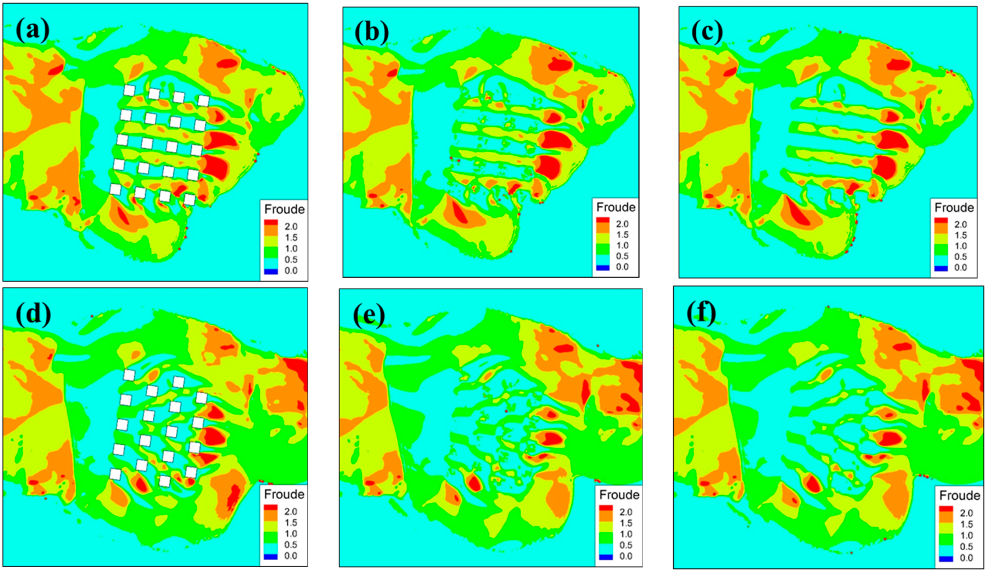
- On comparing the three building representation methods, BB, BH, and BR, the three accuracy indicators, namely, RMSE, PPMCC, and NSE, clearly show that all three methods exhibit significant potential to simulate urban flooding with aligned or staggered building layouts. There is no appropriate method that would offer maximum performance in terms of all three indicators. Analysis of assessment indicators for different layouts of the model city revealed few differences between the three methods. In general, the BR method shows relatively better performance according to the three indicators. Hence, the BR method is deemed suitable for urban flood simulation.
- Numerical models with 1, 2, and 5 cm mesh resolutions for the BH method were established to analyze the influence of the sensitivity of different mesh resolutions. By comparing model performance, we found that the results for the 1 cm mesh resolution are slightly lower than those for the other mesh resolutions. In addition, data oscillation is visible in the results for the 1 cm resolution. Furthermore, RMSEs, PPMCCs, and NSEs were calculated to appraise quantitatively the performance of different mesh resolutions. The results for the 1 cm mesh resolution were found to be better that those for the other mesh resolutions based on the calculated indicators.
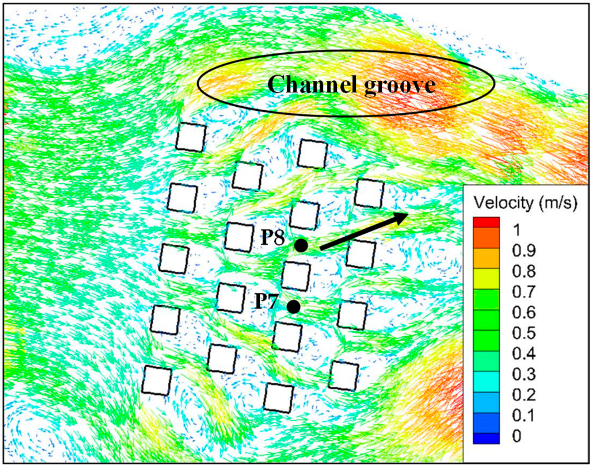
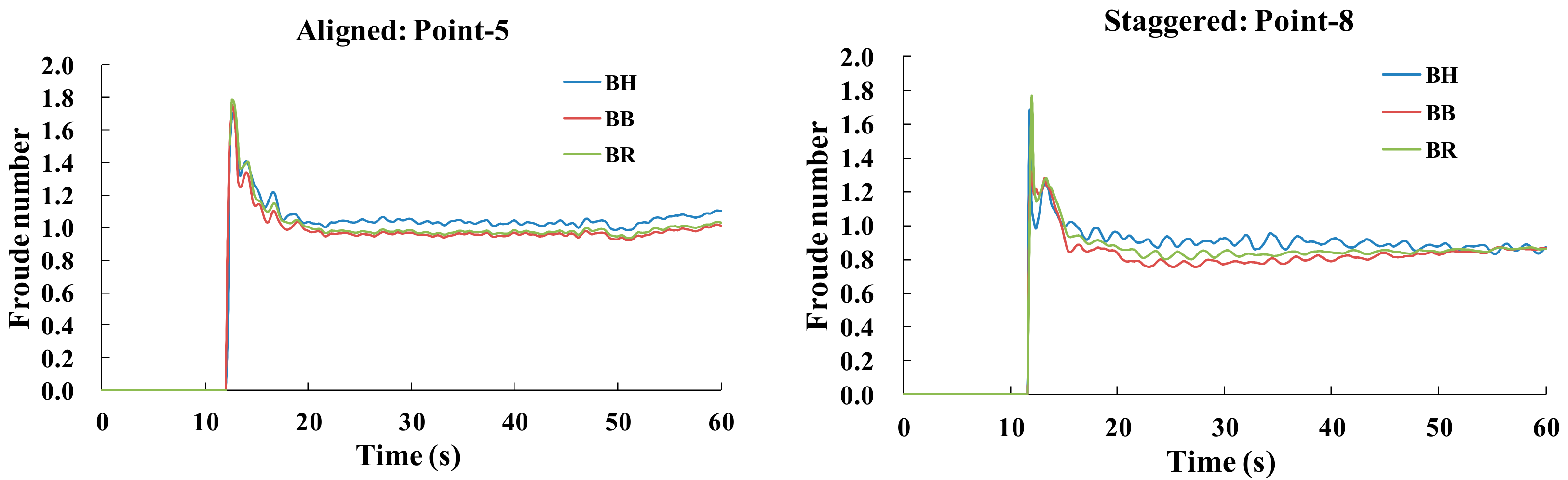
- The discrepancies in the predictions and measurements at gauges P5 and P8 were analyzed and discussed from different perspectives. A possible explanation for these discrepancies is that the water level was influenced by water jump and micro-topography, implying that the classical SWEs have some issues in terms of their hydrostatic and zero vertical velocity hypotheses. Additionally, the mesh resolution, velocity, and Froude number have some influence on the numerical results, and some difficulties in simulating critical flow were experienced. Therefore, modifying and perfecting classical SWEs is an important research objective for future studies.
Author Contributions
Funding
Conflicts of Interest
References
- Begum, R.A.; Sarkar, M.S.K.; Jaafar, A.H.; Pereira, J.J. Toward conceptual frameworks for linking disaster risk reduction and climate change adaptation. Int. J. Disaster Risk Reduct. 2014, 10, 362–373. [Google Scholar] [CrossRef]
- Economic Losses, Poverty & Disasters, CRED 1998–2017; Unites Nations: Geneva, Switzerland, 2017.
- Yuan, Z.; Yan, D.H.; Yang, Z.Y.; Yin, J. Progress of urban flood research and overall handling of urban flood in China. Adv. Mater. Res. Trans. Tech. Pub. 2014, 955, 1881–1888. [Google Scholar] [CrossRef]
- Wang, K.; Wang, L.; Wei, Y.M.; Ye, M. Beijing storm of July 21, 2012: Observations and reflections. Nat. Hazards 2013, 67, 969–974. [Google Scholar] [CrossRef]
- Mignot, E.; Li, X.; Dewals, B. Experimental modelling of urban flooding: A review. J. Hydrol. 2019, 568, 334–342. [Google Scholar] [CrossRef]
- Liu, L.; Sun, J.; Lin, B.; Lu, L. Building performance in dam-break flow—An experimental study. Urban Water J. 2018, 15, 251–258. [Google Scholar] [CrossRef]
- Albano, R.; Sole, A.; Mirauda, D.; Adamowski, J. Modelling large floating bodies in urban area flash-floods via a smoothed particle hydrodynamics model. J. Hydrol. 2016, 541, 344–358. [Google Scholar] [CrossRef]
- Ferrari, A.; Viero, D.P.; Vacondio, R.; Defina, A.; Mignosa, P. Flood inundation modelling in urbanized areas: A mesh-independent porosity approach with anisotropic friction. Adv. Water Resour. 2019, 125, 98–113. [Google Scholar] [CrossRef]
- Viero, D.P. Modelling urban floods using a finite element staggered scheme with an anisotropic dual porosity model. J. Hydrol. 2019, 568, 247–259. [Google Scholar] [CrossRef]
- Wang, Z.L.; Geng, Y.F. Two-dimensional shallow water equations with porosity and their numerical scheme on unstructured grids. Water Sci. Eng. 2013, 6, 91–105. [Google Scholar]
- Guinot, V. Multiple porosity shallow water models for macroscopic modelling of urban floods. Adv. Water Resour. 2012, 37, 40–72. [Google Scholar] [CrossRef]
- Wu, X.; Wang, Z.; Guo, S.; Liao, W.; Zeng, Z.; Chen, X. Scenario-based projections of future urban inundation within a coupled hydrodynamic model framework: A case study in Dongguan City, China. J. Hydrol. 2017, 547, 428–442. [Google Scholar] [CrossRef]
- Zhou, Q.; Yu, W.; Chen, A.S.; Jiang, C.; Fu, G. Experimental assessment of building blockage effects in a simplified urban district. Procedia Eng. 2016, 154, 844–852. [Google Scholar] [CrossRef]
- Schubert, J.E.; Sanders, B.F. Building treatments for urban flood inundation models and implications for predictive skill and modeling efficiency. Adv. Water Resour. 2012, 41, 49–64. [Google Scholar] [CrossRef]
- Kim, B.; Sanders, B.F.; Schubert, J.E.; Famiglietti, J.S. Mesh type tradeoffs in 2D hydrodynamic modeling of flooding with a Godunov-based flow solver. Adv. Water Resour. 2014, 68, 42–61. [Google Scholar] [CrossRef]
- An, H.; Yu, S. Well-balanced shallow water flow simulation on quadtree cut cell grids. Adv. Water Resour. 2012, 39, 60–70. [Google Scholar] [CrossRef]
- Costabile, P.; Macchione, F. Enhancing river model set-up for 2-D dynamic flood modelling. Environ. Model. Softw. 2015, 67, 89–107. [Google Scholar] [CrossRef]
- Seenath, A.; Wilson, M.; Miller, K. Hydrodynamic versus GIS modelling for coastal flood vulnerability assessment: Which is better for guiding coastal management? Ocean Coast Manag. 2016, 120, 99–109. [Google Scholar] [CrossRef]
- Briere, C.; Abadie, S.; Bretel, P.; Lang, P. Assessment of TELEMAC system performances, a hydrodynamic case study of Anglet, France. Coast Eng. 2007, 54, 345–356. [Google Scholar] [CrossRef]
- Barthélémy, S.; Ricci, S.; Morel, T.; Goutal, N.; Le Pape, E.; Zaoui, F. On operational flood forecasting system involving 1D/2D coupled hydraulic model and data assimilation. J. Hydrol. 2018, 562, 623–634. [Google Scholar] [CrossRef]
- Testa, G.; Zuccala, D.; Alcrudo, F.; Mulet, J.; Soares-Frazão, S. Flash flood flow experiment in a simplified urban district. J. Hydraul. Res. 2007, 45, 37–44. [Google Scholar] [CrossRef]
- Hervouet, J.M. Hydrodynamics of Free Surface Flows Modelling with the Finite Element Method; John Wiley & Sons Ltd, The Atrium, Southern Gate: Chichester, UK, 2007; pp. 83–133. [Google Scholar]
- Ata, R. TELEMAC-2D new finite volume schemes for shallow water equations with source terms on 2D unstructured grids. In Proceedings of the XIXth TELEMAC-MASCARET User Conference 2012, St Hugh’s College, Oxford, UK, 18–19 October 2012; pp. 93–98. [Google Scholar]
- Horritt, M.S.; Bates, P.D. Effects of spatial resolution on a raster based model of flood flow. J. Hydrol. 2001, 253, 239–249. [Google Scholar] [CrossRef]
- Yu, D.; Lane, S.N. Urban fluvial flood modelling using a two-dimensional diffusion-wave treatment, part 1: Mesh resolution effects. Hydrol. Process. 2006, 20, 1541–1565. [Google Scholar] [CrossRef]
- Hu, J. A simple numerical scheme for the 2D shallow-water system. arXiv 2018, arXiv:1801.07441. [Google Scholar]
- Schubert, J.E.; Sanders, B.F.; Smith, M.J.; Wright, N.G. Unstructured mesh generation and landcover-based resistance for hydrodynamic modeling of urban flooding. Adv. Water Resour. 2008, 31, 1603–1621. [Google Scholar] [CrossRef]
- Bennett, N.D.; Croke, B.F.; Guariso, G.; Guillaume, J.H.; Hamilton, S.H.; Jakeman, A.J.; Pierce, S.A. Characterising performance of environmental models. Environ. Model. Softw. 2013, 40, 1–20. [Google Scholar] [CrossRef]
- Yu, D.; Lane, S.N. Interactions between subgrid-scale resolution, feature representation and grid-scale resolution in flood inundation modelling. Hydrol. Process. 2011, 25, 36–53. [Google Scholar] [CrossRef]
- Sanders, B.F.; Schubert, J.E.; Gallegos, H.A. Integral formulation of shallow-water equations with anisotropic porosity for urban flood modeling. J. Hydrol. 2008, 362, 19–38. [Google Scholar] [CrossRef]
- Dottori, F.; Todini, E. Testing a simple 2D hydraulic model in an urban flood experiment. Hydrol. Process. 2013, 27, 1301–1320. [Google Scholar] [CrossRef]
- Costabile, P.; Costanzo, C.; Macchione, F. Performances and limitations of the diffusive approximation of the 2-d shallow water equations for flood simulation in urban and rural areas. Appl. Numer. Math. 2017, 116, 141–156. [Google Scholar] [CrossRef]
- Aricò, C.; Sinagra, M.; Begnudelli, L.; Tucciarelli, T. MAST-2D diffusive model for flood prediction on domains with triangular Delaunay unstructured meshes. Adv. Water Resour. 2011, 34, 1427–1449. [Google Scholar] [CrossRef]
- Soares-Frazão, S.; Lhomme, J.; Guinot, V.; Zech, Y. Two-dimensional shallow-water model with porosity for urban flood modelling. J. Hydraul. Res. 2008, 46, 45–64. [Google Scholar] [CrossRef]
- Segura, B.F.; Sanchis, I.C.; Morales, H.M.; González, S.M.; Bussi, G.; Ortiz, E. Using post-flood surveys and geomorphologic mapping to evaluate hydrological and hydraulic models: The flash flood of the Girona River (Spain) in 2007. J. Hydrol. 2016, 541, 310–329. [Google Scholar] [CrossRef]
- Macchione, F.; Costabile, P.; Costanzo, C.; De Lorenzo, G. Extracting quantitative data from non-conventional information for the hydraulic reconstruction of past urban flood events. A case-study. J. Hydrol. 2019, 576, 443–465. [Google Scholar] [CrossRef]
- Martín, V.J.P.; Llasat, M.C. The 1962 flash flood in the Rubí stream (Barcelona, Spain). J. Hydrol. 2018, 566, 441–454. [Google Scholar] [CrossRef]
- Neal, J.C.; Bates, P.D.; Fewtrell, T.J.; Hunter, N.M.; Wilson, M.D.; Horritt, M.S. Distributed whole city water level measurements from the Carlisle 2005 urban flood event and comparison with hydraulic model simulations. J. Hydrol. 2009, 368, 42–55. [Google Scholar] [CrossRef]
- Macchione, F.; Costabile, P.; Costanzo, C.; De Santis, R. Moving to 3-D flood hazard maps for enhancing risk communication. Environ. Model. Softw. 2019, 111, 510–522. [Google Scholar] [CrossRef]
- Leskens, J.G.; Kehl, C.; Tutenel, T.; Kol, T.; De Haan, G.; Stelling, G.; Eisemann, E. An interactive simulation and visualization tool for flood analysis usable for practitioners. Mitig. Adapt. Strat. Glob. Chang. 2017, 22, 307–324. [Google Scholar] [CrossRef]


| Building Layouts | Mesh Resolutions | P3 | P4 | P5 | P6 | P7 | P8 | P9 | P10 | Average |
|---|---|---|---|---|---|---|---|---|---|---|
| Aligned | 1 cm | 1.03 | 1.19 | 0.90 | 0.48 | 0.68 | 1.24 | 0.40 | 0.55 | 0.81 |
| 2 cm | 1.14 | 1.34 | 1.12 | 0.57 | 0.61 | 1.10 | 0.61 | 0.51 | 0.88 | |
| 5 cm | 1.55 | 1.83 | 1.84 | 0.96 | 0.92 | 1.06 | 0.84 | 0.53 | 1.19 | |
| Staggered | 1 cm | 1.06 | 1.21 | 0.97 | 1.02 | 0.44 | 1.59 | 0.47 | 0.47 | 0.90 |
| 2 cm | 1.14 | 1.32 | 1.02 | 1.06 | 0.47 | 1.49 | 0.38 | 0.44 | 0.92 | |
| 5 cm | 1.53 | 1.76 | 1.34 | 1.32 | 0.69 | 1.47 | 0.63 | 0.82 | 1.20 |
| Building Layouts | Mesh Resolutions | P3 | P4 | P5 | P6 | P7 | P8 | P9 | P10 | Average |
|---|---|---|---|---|---|---|---|---|---|---|
| Aligned | 1 cm | 0.84 | 0.83 | 0.83 | 0.91 | 0.84 | 0.79 | 0.94 | 0.89 | 0.86 |
| 2 cm | 0.80 | 0.79 | 0.88 | 0.90 | 0.85 | 0.81 | 0.91 | 0.91 | 0.86 | |
| 5 cm | 0.67 | 0.63 | 0.77 | 0.83 | 0.76 | 0.77 | 0.85 | 0.84 | 0.76 | |
| Staggered | 1 cm | 0.84 | 0.82 | 0.89 | 0.95 | 0.92 | 0.94 | 0.97 | 0.85 | 0.90 |
| 2 cm | 0.81 | 0.78 | 0.86 | 0.91 | 0.91 | 0.93 | 0.95 | 0.86 | 0.88 | |
| 5 cm | 0.67 | 0.63 | 0.72 | 0.81 | 0.82 | 0.83 | 0.84 | 0.80 | 0.77 |
| Building Layouts | Mesh Resolutions | P3 | P4 | P5 | P6 | P7 | P8 | P9 | P10 | Average |
|---|---|---|---|---|---|---|---|---|---|---|
| Aligned | 1 cm | 0.82 | 0.82 | 0.47 | 0.90 | 0.81 | 0.64 | 0.93 | 0.78 | 0.77 |
| 2 cm | 0.77 | 0.77 | 0.19 | 0.86 | 0.84 | 0.72 | 0.84 | 0.81 | 0.72 | |
| 5 cm | 0.58 | 0.57 | −1.18 | 0.60 | 0.64 | 0.74 | 0.68 | 0.80 | 0.43 | |
| Staggered | 1 cm | 0.80 | 0.80 | 0.81 | 0.82 | 0.91 | 0.91 | 0.91 | 0.84 | 0.85 |
| 2 cm | 0.77 | 0.76 | 0.79 | 0.80 | 0.90 | 0.58 | 0.94 | 0.86 | 0.80 | |
| 5 cm | 0.59 | 0.58 | 0.65 | 0.70 | 0.78 | 0.59 | 0.84 | 0.50 | 0.65 |
| Building Layouts | Building Representations | P3 | P4 | P5 | P6 | P7 | P8 | P9 | P10 | Average |
|---|---|---|---|---|---|---|---|---|---|---|
| Aligned | BH method | 1.14 | 1.34 | 1.12 | 0.57 | 0.61 | 1.10 | 0.61 | 0.51 | 0.88 |
| BB method | 1.23 | 1.37 | 1.48 | 0.70 | 0.60 | 0.81 | 0.74 | 0.42 | 0.92 | |
| BR method | 1.11 | 1.24 | 1.29 | 0.51 | 0.51 | 0.85 | 0.51 | 0.39 | 0.80 | |
| Staggered | BH method | 1.14 | 1.32 | 1.02 | 1.06 | 0.47 | 1.49 | 0.38 | 0.44 | 0.92 |
| BB method | 1.26 | 1.40 | 1.25 | 0.74 | 0.35 | 1.27 | 0.31 | 0.50 | 0.89 | |
| BR method | 1.11 | 1.26 | 0.80 | 0.93 | 0.38 | 1.33 | 0.20 | 0.49 | 0.81 |
| Building Layouts | Building Representations | P3 | P4 | P5 | P6 | P7 | P8 | P9 | P10 | Average |
|---|---|---|---|---|---|---|---|---|---|---|
| Aligned | BH method | 0.80 | 0.79 | 0.88 | 0.90 | 0.85 | 0.81 | 0.91 | 0.91 | 0.86 |
| BB method | 0.81 | 0.79 | 0.86 | 0.94 | 0.91 | 0.86 | 0.95 | 0.92 | 0.88 | |
| BR method | 0.81 | 0.81 | 0.90 | 0.94 | 0.91 | 0.89 | 0.96 | 0.91 | 0.89 | |
| Staggered | BH method | 0.81 | 0.78 | 0.86 | 0.91 | 0.91 | 0.93 | 0.95 | 0.86 | 0.88 |
| BB method | 0.81 | 0.77 | 0.88 | 0.93 | 0.95 | 0.96 | 0.98 | 0.87 | 0.89 | |
| BR method | 0.82 | 0.80 | 0.92 | 0.97 | 0.95 | 0.97 | 0.98 | 0.88 | 0.91 |
| Building Layouts | Building Representations | P3 | P4 | P5 | P6 | P7 | P8 | P9 | P10 | Average |
|---|---|---|---|---|---|---|---|---|---|---|
| Aligned | BH method | 0.77 | 0.77 | 0.19 | 0.86 | 0.84 | 0.72 | 0.84 | 0.81 | 0.72 |
| BB method | 0.74 | 0.76 | −0.41 | 0.79 | 0.85 | 0.85 | 0.75 | 0.87 | 0.65 | |
| BR method | 0.79 | 0.80 | −0.07 | 0.89 | 0.89 | 0.83 | 0.88 | 0.89 | 0.74 | |
| Staggered | BH method | 0.77 | 0.76 | 0.79 | 0.80 | 0.90 | 0.58 | 0.94 | 0.86 | 0.80 |
| BB method | 0.72 | 0.74 | 0.69 | 0.90 | 0.94 | 0.69 | 0.96 | 0.82 | 0.81 | |
| BR method | 0.78 | 0.78 | 0.88 | 0.85 | 0.93 | 0.66 | 0.98 | 0.83 | 0.84 |
© 2019 by the authors. Licensee MDPI, Basel, Switzerland. This article is an open access article distributed under the terms and conditions of the Creative Commons Attribution (CC BY) license (http://creativecommons.org/licenses/by/4.0/).
Share and Cite
Li, Z.; Liu, J.; Mei, C.; Shao, W.; Wang, H.; Yan, D. Comparative Analysis of Building Representations in TELEMAC-2D for Flood Inundation in Idealized Urban Districts. Water 2019, 11, 1840. https://doi.org/10.3390/w11091840
Li Z, Liu J, Mei C, Shao W, Wang H, Yan D. Comparative Analysis of Building Representations in TELEMAC-2D for Flood Inundation in Idealized Urban Districts. Water. 2019; 11(9):1840. https://doi.org/10.3390/w11091840
Chicago/Turabian StyleLi, Zejin, Jiahong Liu, Chao Mei, Weiwei Shao, Hao Wang, and Dianyi Yan. 2019. "Comparative Analysis of Building Representations in TELEMAC-2D for Flood Inundation in Idealized Urban Districts" Water 11, no. 9: 1840. https://doi.org/10.3390/w11091840
APA StyleLi, Z., Liu, J., Mei, C., Shao, W., Wang, H., & Yan, D. (2019). Comparative Analysis of Building Representations in TELEMAC-2D for Flood Inundation in Idealized Urban Districts. Water, 11(9), 1840. https://doi.org/10.3390/w11091840