Article

Analysis of the Slope Response to an Increase in Pore Water Pressure Using the Material Point Method

Department of Civil Engineering, University of Calabria, Rende, 87036 Cosenza, Italy
*
Author to whom correspondence should be addressed.
Water 2019, 11(7), 1446; https://doi.org/10.3390/w11071446
Submission received: 29 May 2019 / Revised: 29 June 2019 / Accepted: 9 July 2019 / Published: 12 July 2019
(This article belongs to the Special Issue Water-Induced Landslides: Prediction and Control)

Abstract

:
Traditional numerical methods, such as the finite element method or the finite difference method, are generally used to analyze the slope response in the pre-failure and failure stages. The post-failure phase is often ignored due to the unsuitability of these methods for dealing with problems involving large deformations. However, an adequate analysis of this latter stage and a reliable prediction of the landslide kinematics after failure are very useful for minimizing the risk of catastrophic damage. This is generally the case of the landslides triggered by an excess in pore water pressure, which are often characterized by high velocity and long run-out distance. In the present paper, the deformation processes occurring in an ideal slope owing to an increase in pore water pressure are analyzed using the material point method (MPM) that is a numerical technique capable of overcoming the limitations of the above-mentioned traditional methods. In particular, this study is aimed to investigate the influence of the main involved parameters on the development of a slip surface within the slope, and on the kinematics of the consequent landslide. The obtained results show that, among these parameters, the excess water pressure exerts the major influence on the slope response. A simple equation is also proposed for a preliminary evaluation of the run-out distance of the displaced soil mass.

1. Introduction

Excess pore water pressure, due for example to prolonged and heavy rainfall, groundwater level rising, or earthquakes, generally exerts a strong influence on the slope stability. Following the scheme originally introduced by the authors of [1,2], an increase in pore pressure induces a deformation process in the slope (pre-failure stage), which could lead to the slope collapse (failure stage) and the occurrence of large displacements of the unstable soil mass until a new condition of equilibrium is reached (post-failure stage). Some typical situations are schematized in Figure 1. Specifically, Figure 1a shows a cover soil overlaying a geological formation with much higher permeability and greater mechanical properties than the former soil. In these circumstances, an excess in pore water pressure owing to an increase of the hydraulic head in the upper portion of the slope (for example, due to rain infiltration) could lead to the instability of the cover soil with a slip surface located at the interface of the two materials. Figure 1b shows a slope where a soil layer with low permeability (for example, a clayey layer) is interbedded in a geological formation characterized by a much higher hydraulic conductibility than that of the soil layer. An excess in pore water pressure occurring in the lower portion of the slope (for example, due to water recharge) could trigger a landslide in the portion of the slope above the soil layer. Similar considerations can be made for the dual situation shown in Figure 1c, where a saturated soil layer (for example, a sandy layer) under pressure is interbedded in a much less permeable formation. Case studies similar to those above-described are documented in several published papers [3,4,5].
Generally, stability of such slopes is assessed by analyzing only the deformation processes that occur in the pre-failure and failure stages. Simplified approaches [6,7,8,9,10,11] and numerical methods based on the assumption of small strains [12,13,14,15,16,17,18,19,20,21] are often used for this aim. On the contrary, the post-failure stage is usually ignored owing to the unsuitability of the above-mentioned methods to deal with problems involving large deformations. However, a prediction of the landslide kinematics after failure is very useful to minimize the risk connected with the occurrence of landslides or to establish the most suitable mitigation measures for land protection. Modelling large deformations requires the use of alternative methods that often combine the performance of different numerical techniques [22,23]. Most methods proposed in the literature refer to two distinct approaches: the discrete approach and the continuum one. The distinct element method (DEM) falls into the former category. Application of this method to simulate the occurrence of landslides and their evolution can be found in several studies [24,25,26]. The smoothed particle hydrodynamics method (SPH) [27,28] and the material point method (MPM) [29,30,31] are the most used continuum approaches for modelling landslide problems. A comprehensive review of these methods was presented by [32] who also highlighted the great capability of MPM for analysing the stability of slopes and their post-failure response. In this latter method, a continuum is discretized into two different frames: a set of Lagrangian points, called material points, and a fixed computational mesh. Consequently, the method combines the advantages of the Eulerian and Lagrangian formulations and prevents numerical drawbacks due to mesh distortion. In addition, the contact problems between different bodies are automatically solved [4]. Therefore, MPM is suitable for simulating extreme events which involve large displacements, such as the post-failure phase of landslides [32,33,34].
In this paper, MPM is used to simulate the deformation processes occurring in the pre-failure, failure, and post-failure phases of landslides triggered by a change in pore water pressure. Referring to an ideal slope consisting of cohesionless soils under drained conditions, a theoretical study is performed. Particularly, the influence of the main parameters involved in the development of a slip surface within the slope and the kinematics of the landslide after failure is investigated in detail. Moreover, a very simple equation is proposed for predicting the run-out distance of the displaced soil mass as a function of these parameters.

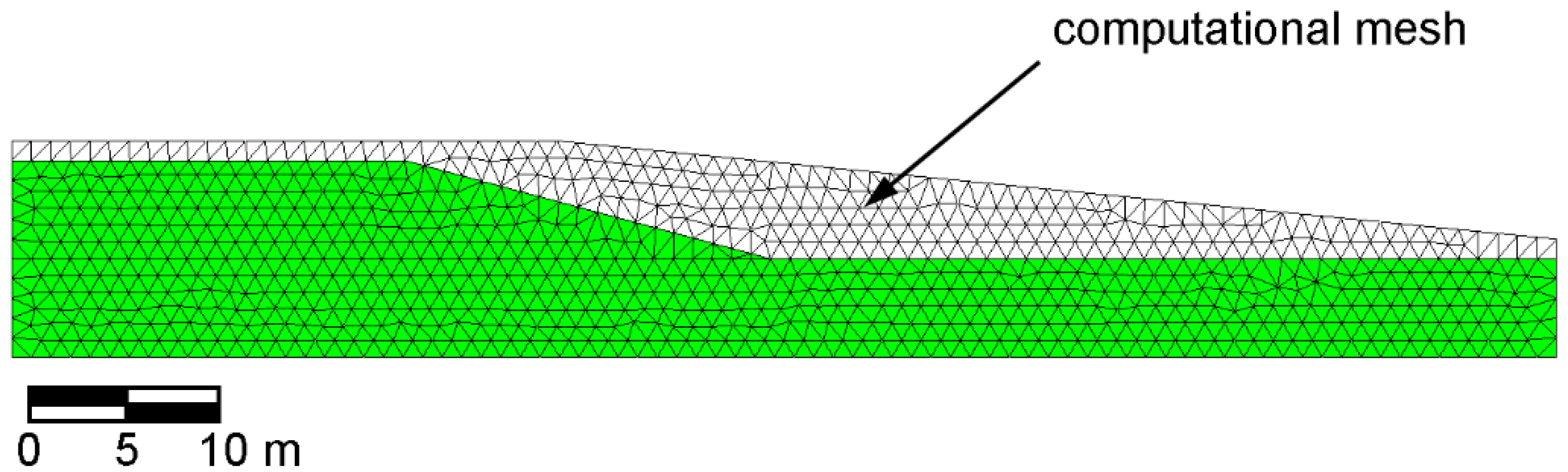
2. Material Point Method
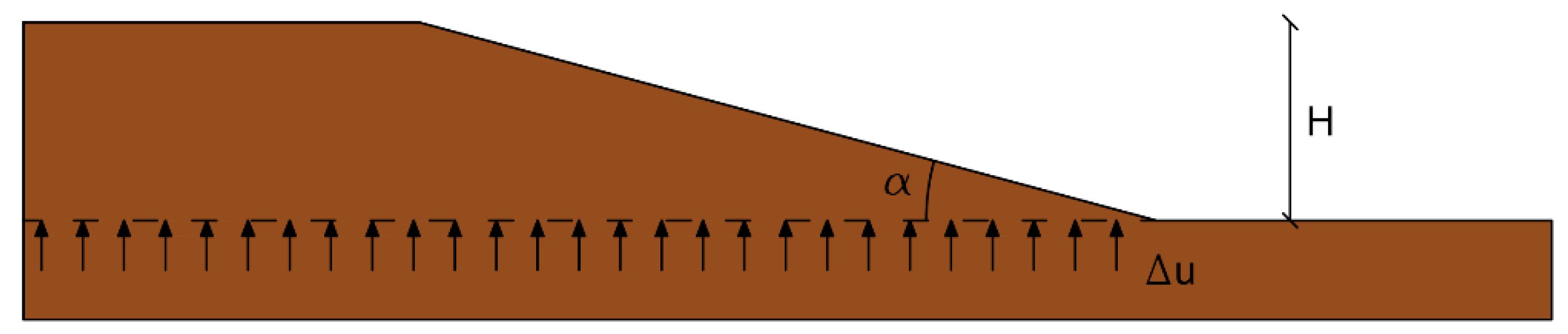
The material point method was first introduced by the authors of [35]. In the standard approach, a continuum is discretized by a set of subdomains (Figure 2). The mass of each subdomain is assumed to be concentrated in a Lagrangian point (called the material point) that carries also other proprieties of the subdomain, such as velocities, stresses, strains, and material parameters as well as external loads. Additionally, a background fixed Eulerian mesh is adopted to solve the governing equations and to perform the required differentiation and integration operations. This mesh covers the full domain of the problem under consideration. Empty elements are also required outside the initial geometry in order to capture the material points that will leave the original position. Therefore, the sizes of the computational mesh are larger than those of the initial geometry. The occurrence of large displacements is simulated updating the position of the material points moving through the fixed mesh.
A scheme of the calculation procedure is shown in Figure 3. At a given time, any information stored in the material points is mapped to the computational mesh (Figure 3a). Interpolation shape functions provide the relationship between material points and nodes. Then, the unknown variables are calculated by solving the governing equations (Figure 3b), and the resulting acceleration, velocity, and displacement of the material points are updated (Figure 3c). In addition, strains and stresses are evaluated using an appropriate constitutive model. The position of the material points is also updated after a mesh adjustment (Figure 3d). Finally, time is incremented by a time step Δt, and the solution procedure is applied at the next time step.
Two different approaches have been developed in the last years: the single-layer approach [36,37,38,39] and the multi-layer one [40,41,42,43]. A scheme of these approaches is shown in Figure 4.
In the former approach, a saturated soil is discretized by a set of material points. Each material point represents both solid phase and water phase. The material points move attached to the solid skeleton giving a Lagrangian description of the solid phase motion. Water motion occurs simultaneously with that of the solid phase. In the multi-layer approach, solid and fluid phases are represented separately by means of different sets of material points. Each material point carries only information of the phase that it represents. Therefore, this latter approach is suitable to model problems where pore fluids move separately from the solid phase. However, the number of material points required to discretize a porous domain considerably increases compared to the single-layer formulation, making the multi-layer formulation computationally much more expensive than the multi-layer one. The approach considered in the present paper is the single-layer one. In particular, the two-phase single-point formulation is used, in which all information about a saturated porous medium is carried by one set of material points, whereas pore water pressure is an additional variable [44]. The reason for using this formulation is that the effects of the relative motion between solid and water phases should not be significant for the problem considered in the present study [4,45]. In addition, as already said, this choice considerably reduces the computational costs with respect to the multi-layer formulation. The analyses presented in the following sections have been carried out using the ANURA3D code, developed by the ANURA3D MPM Research Community [46].

3. Parametric Study

Figure 5 shows an ideal slope the geometry of which is defined by two parameters: inclination angle, α, and slope height, H. The slope consists of a saturated soil with a linear elastic perfectly plastic Mohr-Coulomb constitutive model and non-associated flow rule. The soil is purely frictional. In addition, it is assumed that no change in the shear strength parameters occurs with increasing strain. Therefore, the case of the soils with strain-softening behavior is not considered in the present study. The soil parameters used in the analysis are indicated in Table 1, where γ is the unit weight, E’ is Young’s modulus, ν’ is Poisson’s ratio, c’ is the effective cohesion, φ’ is the shearing resistance angle, ψ is the angle of dilation, and k is the coefficient of permeability. Considering that the numerical simulations are carried out under drained loading, a high value of the coefficient of permeability is assumed. As explained below, this choice of k also satisfies the stability condition of the solution and leads to a reduction of the calculation time. The authors have also found that a different choice of E’ and ν’ (which satisfies the above-mentioned stability condition) does not significantly affect the conclusions of the present study. Finally, different values of φ’ are assumed in the calculations, as indicated in Table 1.
The analysis is carried out under plain-strain conditions by using a computational mesh made up of triangular elements with an average size of 1 m (Figure 6). Initially, three material points are distributed within each element. Boundary conditions are simulated by rollers located on the left and right sides of the model to constrain the horizontal displacement, and by hinges at the bottom of the mesh where both vertical and horizontal displacements are prevented. A boundary condition is also enforced at the top of the mesh to fix the vertical displacement.
The initial stress state of the slope is reproduced using the well-known gravity loading procedure, with the soil that is assumed to be fully saturated. Afterwards, an excess of pore water pressure, Δu, is imposed at the slope base (Figure 5) owing to which motion of the unstable soil mass starts or accelerates if motion is in progress. A similar scheme was considered by the authors of [32] to simulate successfully the Selborne slope failure. Excess pore water pressure could be due to a rapid water recharge or a phreatic level rise, as occurs in the situations schematized in Figure 1. Although in these situations, an increase in pore pressure is favoured by the presence of soils with different permeability, slope failure involves a homogeneous soil like in the slope schematized in Figure 5.
Since ANURA3D uses an explicit dynamic formulation to solve the governing equations, the solution is conditionally stable, i.e., a time-step less than a critical value must be used in the calculations. This critical value can be evaluated according to the Courant–Friedrichs–Levy condition [47]. For the case considered in the present study, it was found that a value of Δt = 0.01 s is sufficient to satisfy this condition. In addition, this value reduces the calculation time.

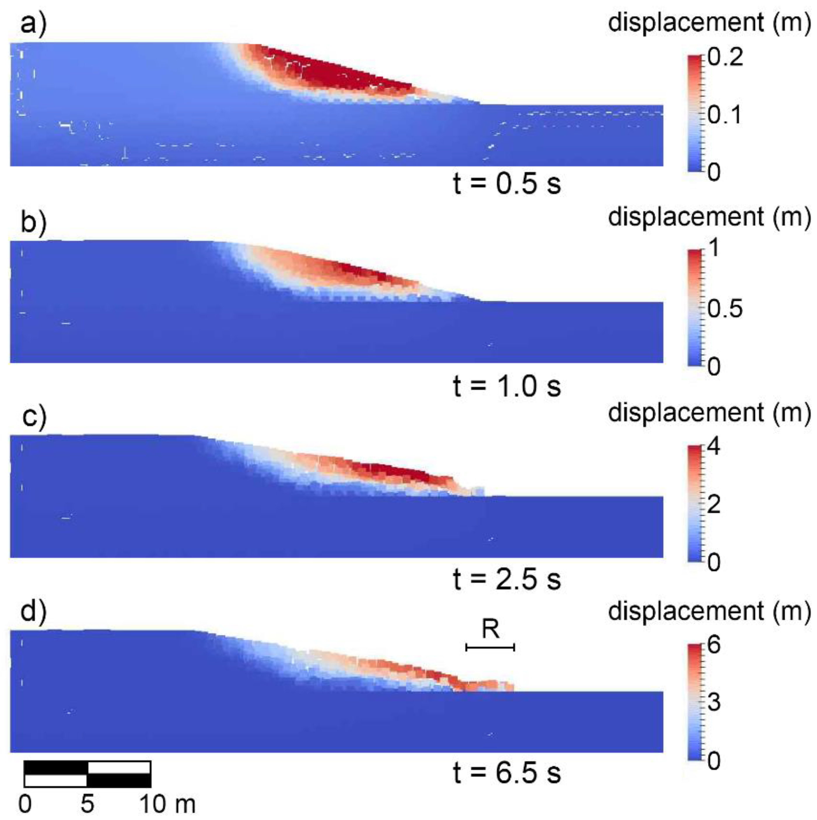
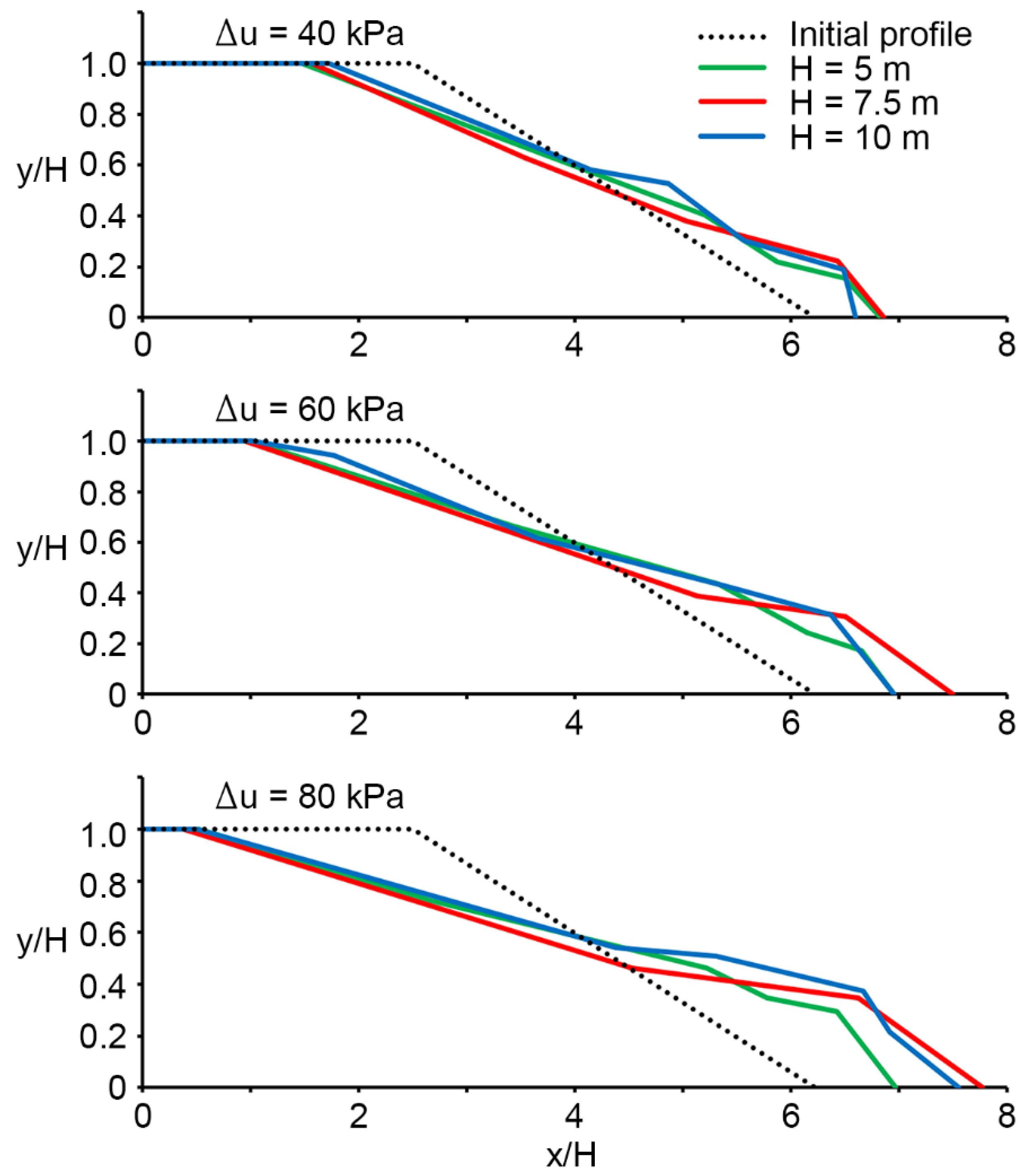
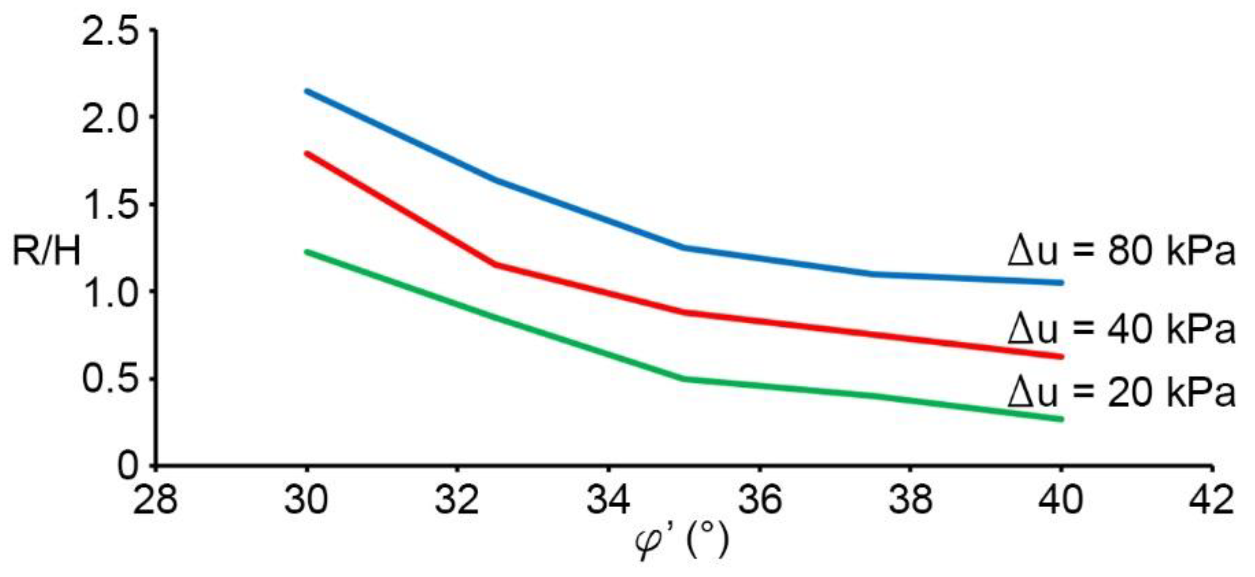
Results and Discussion

In this section, a study is carried out to analyze the influence of the main involved parameters on the slope response. These parameters are slope height H, inclination angle α, soil shearing resistance angle φ’, and excess pore water pressure Δu. The values considered for H range between 5 m and 10 m, and those for α between 10° and 20°. In addition, φ’ varies from 30° to 40° and Δu from 20 kPa to 80 kPa.
The results presented in Figure 7 refer to the case with H = 5 m, Δu = 40 kPa, φ’ = 35°, and α = 15°, and show the soil displacements calculated at four different times after imposing an excess in pore pressure at the depth indicated in Figure 5. The safety factor of this slope, SF, is equal to 2.70 or 1.13 when the soil is assumed dry or fully saturated, respectively. Therefore, the slope is initially stable. These values of SF have been obtained using the phi/c reduction procedure implemented in the finite element code PLAXIS 2D [48].
As can be observed, a slip surface develops within the slope at depths less than that where Δu is imposed (Figure 7a). When this slip surface is completely developed (Figure 7b), the slope collapses and the unstable soil mass moves downstream. Displacements undergone by the material points define the kinematics of the landslide. With increasing time, displacement increases (Figure 7c) until all material points attain a new condition of equilibrium (Figure 7d). At this time, it is possible to detect the final post-failure profile of the landslide and the run-out distance R, which is defined as the distance between the tip of the displaced material and the toe of the slope before failure (Figure 7d). In conclusion, using MPM all phases (pre-failure, failure, and post-failure) of a landslide can be effectively simulated.
Figure 8 compares the final profile of the landslide for a slope initially with α = 15°, φ’ = 35° and different values of H and Δu. The coordinates of the profile are plotted in dimensionless form with respect to H. For the sake of completeness, the initial configuration of the slope is also indicated in Figure 8 by a dashed line. The results show that, for a given value of Δu, the dimensionless post-failure profile and the associated run-out distance are slightly affected by the initial height of the slope. On the contrary, substantial differences in the final geometry of the landslide can be observed when a different value of Δu is considered. Specifically, the greater is Δu, the larger are the accumulation and depletion zones of the displaced material. Similar considerations can be made about the shape and position of the slip surface, which are essentially unchanged when a different value of H is considered (Figure 9), but strongly depend on the imposed Δu (Figure 10).
In particular, Figure 10 shows that the slip surface enlarges upstream with increasing Δu. In other words, the greater is Δu, the greater is the volume of the unstable soil mass. Numerical simulations are also performed using different values of α and φ’, in order to investigate their influence on the location of the slip surface and the final configuration of the landslide.
Figure 11 shows the location of the slip surface and the post-failure profile obtained for the case with H = 5 m, φ’ = 35°, Δu = 40 kPa, and for two values of α. The slip surface moves upstream when a greater value of α is considered. In addition, the greater is α, the larger is the volume of the displaced material (Figure 11). A similar trend can be observed when a lower value of the angle of shearing resistance is assumed (Figure 12).
Finally, the influence of α, φ’ and Δu on the dimensionless run-out distance, R/H, is documented in Figure 13 and Figure 14. The resulting values of R/H are also shown in Table 2. As expected, R/H decreases with increasing φ’, and increases with an increase in α and Δu.
On the basis of all these results, the following equation is proposed to relate R/H to α, φ’, and Δu:
R H = Δ u a e b tan φ
where Δu is expressed in kPa. The coefficients a and b appearing in Equation (1) were evaluated using a trial-and-error procedure. Specifically, for any assumed value of the slope angle, these coefficients were determined as those providing the best agreement between Equation (1) and the numerical simulations. Finally, the expressions relating a and b to α were obtained by fitting the available results. These expressions are:
a = 350 e 7 tan α
b = 3 20 ( tan α ) 3 2
A comparison of the values of R/H calculated using Equation (1) to those obtained using MPM is shown in Figure 15. Considering that almost all the results are arranged close to a 45° steep straight line, it can be concluded that the values of R/H calculated using the proposed equations and those derived from the numerical simulations are in fairly good agreement, in spite of the complexity of the problem under consideration. The predictive capacity of the proposed equation is better for low values of R/H. On the contrary, some discrepancies between simplified and numerical prediction occur at high values of R/H. Although affected by these limitations, Equation (1) could be useful for an approximate prediction of the run-out distance of landslides in situations similar to those considered in the present study.

4. Conclusions

In the present paper, the material point method is used to analyze the response of slopes to an excess in pore water pressure due for example to a water recharge or a phreatic level rise, as often occurs in several real situations. Referring to an ideal slope consisting of cohesionless soils under drained conditions, at the base of which an excess in pore water pressure occurs, attention is mainly focused on the development of a slip surface within the slope in the pre-failure phase, and the kinematics of the landslide in the post-failure stage. A parametric study is carried out to analyze the influence of the main involved parameters on the shape and position of the slip surface as well as on the final configuration of the displaced material and its run-out distance. The results have shown that, although all these parameters affect the slope response, the excess pore pressure exerts the greatest influence on the results. Finally, a simple equation is proposed for an approximate prediction of the run-out distance of the unstable soil mass in situations similar to those considered in the present study.

Author Contributions

A.T. designed the analyses and wrote the paper; E.C. directed the preparation of the article and revised it; L.P. performed the numerical analyses using the ANURA3D code. All authors contributed equally to the preparation of this work.

Funding

This research received no external funding

Conflicts of Interest

The authors declare no conflict of interest.

References

  1. Vaunat, J.; Leroueil, S.; Faure, R. Slope movements: a geotechnical perspective. In Proceedings of the 7th Congress International Association of Engineering Geology, Lisbon, Portugal, 5–9 September 1994; pp. 1637–1646. [Google Scholar]
  2. Leroueil, S.; Vaunat, J.; Picarelli, L.; Locat, J.; Faure, J.; Lee, H. A geotechnical characterization of slope movements. In Proceedings of the 7th International Symposium on Landslides, Trondheim, Norway, 17–21 June 1996; Balkema: Rotterdam, The Netherlands; pp. 53–74. [Google Scholar]
  3. Cascini, L.; Cuomo, S.; Sorbino, G. Flow-like mass movements in pyroclastic soils: remarks on the modelling of the triggering mechanism. Italian Geotech. J. 2005, 4, 11–31. [Google Scholar]
  4. Yerro, A.; Alonso, E.; Pinyol, N. Run-out of landslides in brittle soils. Comput. Geotech. 2016, 80, 427–439. [Google Scholar] [CrossRef] [Green Version]
  5. Conte, E.; Donato, A.; Pugliese, L.; Troncone, A. Analysis of the Maierato landslide (Calabria, Southern Italy). Landslides 2018, 15, 1935–1950. [Google Scholar] [CrossRef]
  6. Duncan, J.M. State of the Art: Limit Equilibrium and Finite-Element Analysis of Slopes. J. Geotech. Eng. 1996, 122, 577–596. [Google Scholar] [CrossRef]
  7. Corominas, J.; Moya, J.; Ledesma, A.; Lloret, A.; Gili, J.A. Prediction of ground displacements and velocities from groundwater level changes at the Vallcebre landslide (Eastern Pyrenees, Spain). Landslides 2005, 2, 83–96. [Google Scholar] [CrossRef]
  8. Conte, E.; Troncone, A. A method for the analysis of soil slips triggered by rainfall. Géotechnique 2012, 62, 187–192. [Google Scholar] [CrossRef]
  9. Conte, E.; Troncone, A. Stability analysis of infinite clayey slopes subjected to pore pressure changes. Géotechnique 2012, 62, 87–91. [Google Scholar] [CrossRef]
  10. Conte, E.; Troncone, A.; Conte, E.; Troncone, A. A performance-based method for the design of drainage trenches used to stabilize slopes. Eng. Geol. 2018, 239, 158–166. [Google Scholar] [CrossRef]
  11. Conte, E.; Donato, A.; Troncone, A. A simplified method for predicting rainfall-induced mobility of active landslides. Landslides 2017, 14, 35–45. [Google Scholar] [CrossRef]
  12. Dounias, G.T.; Potts, D.M.; Vaughan, P.R. Finite element analysis of progressive failure of Carsington embankment. Géotechnique 1990, 40, 79–101. [Google Scholar]
  13. Alonso, E.E.; Gens, A.; Delahaye, C.H. Influence of rainfall on the deformation and stability of a slope in overconsolidated clays: a case study. Hydrogeol. J. 2003, 11, 174–192. [Google Scholar] [CrossRef] [Green Version]
  14. Troncone, A. Numerical analysis of a landslide in soils with strain-softening behaviour. Géotechnique 2005, 55, 585–596. [Google Scholar] [CrossRef]
  15. Lollino, P.; Santaloia, F.; Amorosi, A.; Cotecchia, F. Delayed failure of quarry slopes in stiff clays: the case of the Lucera landslide. Géotechnique 2011, 61, 861–874. [Google Scholar] [CrossRef]
  16. Fernàndez-Merodo, J.A.; Garcìa-Davalillo, J.C.; Herrera, G.; Mira, P.; Pastor, M. 2D viscoplastic finite element modelling of slow landslides: the Portalet case study (Spain). Géotechnique 2014, 11, 29–42. [Google Scholar] [CrossRef]
  17. Troncone, A.; Conte, E.; Donato, A. Two and three-dimensional numerical analysis of the progressive failure that occurred in an excavation-induced landslide. Eng. Geol. 2014, 183, 265–275. [Google Scholar] [CrossRef]
  18. Conte, E.; Donato, A.; Troncone, A. A finite element approach for the analysis of active slow-moving landslides. Landslides 2014, 11, 723–731. [Google Scholar] [CrossRef]
  19. Griffiths, D.V.; Lane, P.A. Slope stability analysis by finite elements. Géotechnique 1999, 49, 387–403. [Google Scholar] [CrossRef]
  20. Potts, D.M.; Zdravkovic, L. Finite Element Analysis in Geotechnical Engineering: Application; Thomas Telford: London, UK, 2001. [Google Scholar]
  21. Picarelli, L.; Urciuoli, G.; Russo, C. Effect of groundwater regime on the behaviour of clayey slopes. Can. Geotech. J. 2004, 41, 467–484. [Google Scholar] [CrossRef]
  22. Hung, C.; Liu, C.-H.; Chang, C.-M. Numerical Investigation of Rainfall-Induced Landslide in Mudstone Using Coupled Finite and Discrete Element Analysis. Geofluids 2018, 2018, 1–15. [Google Scholar] [CrossRef] [Green Version]
  23. Chen, X.; Zhang, L.; Chen, L.; Li, X.; Liu, D. Slope stability analysis based on the Coupled Eulerian-Lagrangian finite element method. Bull. of Eng. Geology and the Environ. 2019, 1–13. [Google Scholar] [CrossRef]
  24. Lin, C.-H.; Lin, M.-L. Evolution of the large landslide induced by Typhoon Morakot: A case study in the Butangbunasi River, southern Taiwan using the discrete element method. Eng. Geol. 2015, 197, 172–187. [Google Scholar] [CrossRef]
  25. Calvetti, F.; di Prisco, C.; Vairaktaris, E. DEM assessment of impact forces of dry granular masses on rigid barriers. Acta Geotech. 2017, 12, 129–144. [Google Scholar] [CrossRef]
  26. Scaringi, G.; Fan, X.; Xu, Q.; Liu, C.; Ouyang, C.; Domènech, G.; Yang, F.; Dai, L. Some considerations on the use of numerical methods to simulate past landslides and possible new failures: the case of the recent Xinmo landslide (Sichuan, China). Landslides 2018, 15, 1359–1375. [Google Scholar] [CrossRef]
  27. Pirulli, M.; Pastor, M. Numerical study on the entrainment of bed material into rapid landslides. Géotechnique 2012, 62, 959–972. [Google Scholar] [CrossRef]
  28. Li, L.; Wang, Y.; Zhang, L.; Choi, C.; Ng, C.W.W. Evaluation of Critical Slip Surface in Limit Equilibrium Analysis of Slope Stability by Smoothed Particle Hydrodynamics. Int. J. Geéomeéch. 2019, 19. [Google Scholar] [CrossRef]
  29. Alonso, E.; Zabala, F. Progressive failure of Aznalcóllar dam using the material point method. Géotechnique 2011, 61, 795–808. [Google Scholar]
  30. Zhang, X.; Chen, Z.; Liu, Y. The Material Point Method: A Continuum-Based Particle Method for Extreme Loading Cases; Elsevier: London, UK, 2017. [Google Scholar]
  31. Fern, J.; Rohe, A.; Soga, K.; Alonso, A. The Material Point Method for Geotechnical Engineering. A Practical Guide; CRC Press: Boca Raton, FL, USA, 2019. [Google Scholar]
  32. Soga, K.; Alonso, E.; Yerro, A.; Kumar, K.; Bandara, S. Trends in large-deformation analysis of landslide mass movements with particular emphasis on the material point method. Géotechnique 2016, 66, 1–26. [Google Scholar] [CrossRef]
  33. Conte, E.; Pugliese, L.; Troncone, A. Post-failure stage simulation of a landslide using the material point method. Eng. Geol. 2019, 253, 149–159. [Google Scholar] [CrossRef]
  34. Yerro, A.; Soga, K.; Bray, J.D. Runout evaluation of Oso landslide with the material point method. Can. Geotech. J. 2018, 1–14. [Google Scholar] [CrossRef]
  35. Sulsky, D.; Chen, Z.; Schreyer, H. A particle method for history-dependent materials. Comput. Methods Appl. Mech. Eng. 1994, 118, 179–196. [Google Scholar] [CrossRef]
  36. Ceccato, F.; Beuth, L.; Simonini, P. Analysis of Piezocone Penetration under Different Drainage Conditions with the Two-Phase Material Point Method. J. Geotech. Geoenvironmental Eng. 2016, 142, 4016066. [Google Scholar] [CrossRef]
  37. Galavi, V.; Beuth, L.; Coelho, B.Z.; Tehrani, F.S.; Hölscher, P.; Van Tol, F. Numerical Simulation of Pile Installation in Saturated Sand Using Material Point Method. Procedia Eng. 2017, 175, 72–79. [Google Scholar] [CrossRef]
  38. Fern, E.J.; de Lange, D.A.; Zwanenburg, C.; Teunissen, J.A.M.; Rohe, A.; Soga, K. Experimental and numerical investigations of dyke failures involving soft materials. Eng. Geol. 2016, 219, 130–139. [Google Scholar] [CrossRef] [Green Version]
  39. Yerro, A.; Pinyol, N.M.; Alonso, E.E. Internal progressive failure in deep-seated landslides. Rock Mechanics Rock Eng. 2016, 49, 2317–2332. [Google Scholar] [CrossRef]
  40. Martinelli, M.; Rohe, A. Modelling fluidization and sedimentation using material point method. In Proceedings of the 1st Pan-American Congress on Computational Mechanics, Buenos-Aires, Argentina, 27–29 April 2015; pp. 1–12. [Google Scholar] [CrossRef]
  41. Bolognin, M.; Martinelli, M.; Bakker, K.J.; Jonkman, S.N. Validation of material point method for soil fluidisation analysis. J. Hydrodyn. 2017, 29, 431–437. [Google Scholar] [CrossRef]
  42. Martinelli, M.; Rohe, A.; Soga, K. Modeling Dike Failure using the Material Point Method. Procedia Eng. 2017, 175, 341–348. [Google Scholar] [CrossRef]
  43. Ceccato, F.; Yerro, A.; Martinelli, M. Modelling soil-water interaction with the material point method. Evaluation of single-point and double-point formulations. In Proceedings of the Numerical Methods in Geotechnical Engineering IX, Porto, Portugal, 25–27 June 2018; Informa UK Limited: Colchester, UK, 2018; Volume 1, pp. 351–357. [Google Scholar]
  44. Yerro, A.; Alonso, E.; Pinyol, N. The material point method for unsaturated soils. Géotechnique 2015, 65, 201–217. [Google Scholar] [CrossRef] [Green Version]
  45. Alonso, E.E.; Yerro, A.; Pinyol, N.M. Recent developments of the Material Point Method for the simulation of landslides. IOP Conf. Ser. Earth Environ. Sci. 2015, 26, 12003. [Google Scholar] [CrossRef]
  46. Anura3D MPM Research Community. Available online: www.anura3d.com (accessed on 10 July 2019).
  47. Courant, R.; Friedrichs, K.; Lewy, H. On the Partial Difference Equations of Mathematical Physics. IBM J. Res. Dev. 1967, 11, 215–234. [Google Scholar] [CrossRef]
  48. PLAXIS 2D Reference Manual 2019. Available online: www.plaxis.com/support/manuals/plaxis-2d-manuals/ (accessed on 28 June 2019).
Figure 1. Some typical situations in which an excess of pore water pressure could trigger a landslide: (a) A slope with a low permeable cover soil; (b) A slope with a low permeable soil layer; (c) A slope with a high permeable soil layer. Δu: excess pore water pressure; k1, k2: coefficient of permeability; Δh: increase in hydraulic head.
Water 11 01446 g001
Figure 2. Scheme of the spatial discretization of the material point method (MPM).
Water 11 01446 g002
Figure 3. Computational scheme of MPM: (a) Map information from material points to grid nodes; (b) Solution of the governing equations at the nodes; (c) Update of the material point information; (d) Update of the material point position.
Water 11 01446 g003
Figure 4. Scheme of the different approaches of the MPM (adapted from [44]).
Water 11 01446 g004
Figure 5. Slope model considered in the analysis. α: inclination angle; H: slope height.
Water 11 01446 g005
Figure 6. Mesh employed in the analysis.
Water 11 01446 g006
Figure 7. Total displacement of the material points at different times, for the case with: φ’ = 35°; α = 15°; H = 5 m, and Δu = 40 kPa. (a) t = 0.5 s; (b) t = 1.0 s; (c) t = 2.5 s; (d) t = 6.5 s. R: run-out distance.
Water 11 01446 g007
Figure 8. Dimensionless post-failure profiles for the case with α = 15°, φ’ = 35° and different values of Δu and H.
Water 11 01446 g008
Figure 9. Location of the slip surface in dimensionless coordinates, for the case with α = 15°, φ’ = 35°, Δu = 40 kPa, and different values of H.
Water 11 01446 g009
Figure 10. Location of the slip surface in dimensionless coordinates, for the case with α = 15°, φ’ = 35°, and different values of Δu.
Water 11 01446 g010
Figure 11. Dimensionless post-failure profile and slip surface location for the case with H = 5 m, φ’ = 35°, Δu = 40 kPa, α = 10° (a), and α = 20° (b).
Water 11 01446 g011
Figure 12. Dimensionless post-failure profile (a) and slip surface location (b) for the case with H = 5 m, α = 15°, Δu = 40 kPa, and different values of φ’.
Water 11 01446 g012
Figure 13. Dimensionless run-out distance, R/H, versus φ’, for α = 20° and some values of Δu.
Water 11 01446 g013
Figure 14. Dimensionless run-out distance, R/H, versus φ’, for Δu = 60 kPa and some values of α.
Water 11 01446 g014
Figure 15. Comparison of the dimensionless run-out distance evaluated using Equation (1) to that provided by MPM. R/H: dimensionless run-out distance.
Water 11 01446 g015
Table 1. Soil properties used in the analysis. γ: unit weight, E’: Young’s modulus; ν’: Poisson’s ratio; φ’: shearing resistance angle; ψ: angle of dilation; k: coefficient of permeability; c’: effective cohesion.
Materialγ (kN/m3)E’ (kPa)ν’φ’ (°)c’ (kPa)ψ (°)k (m/s)
Soil2025,0000.330–40000.01
Table 2. Values of the dimensionless run-out, R/H, calculated using the MPM. φ’: shearing resistance angle; α: inclination angle; Δu: excess pore water pressure.
α = 10°α = 15°α = 20°
φ’ (°)Δu
20 kPa
Δu
40 kPa
Δu
60 kPa
Δu
80 kPa
Δu
20 kPa
Δu
40 kPa
Δu
60 kPa
Δu
80 kPa
Δu
20 kPa
Δu
40 kPa
Δu
60 kPa
Δu
80 kPa
300.120.180.210.360.190.790.910.970.921.431.822.15
350.060.060.140.150.050.600.730.750.440.881.171.25
400.030.040.100.110.040.310.570.610.260.631.101.13

