Article

Optimization of Pressurized Tree-Type Water Distribution Network Using the Improved Decomposition–Dynamic Programming Aggregation Algorithm

1
School of Environmental Science and Engineering, Yangzhou University, Yangzhou 225127, China
2
School of Hydraulic Energy and Power Engineering, Yangzhou University, Yangzhou 225127, China
3
School of Construction Equipment and Municipal Engineering, Jiangsu Vocational Institute of Architectural Technology, Xuzhou 221008, China
*
Authors to whom correspondence should be addressed.
Water 2019, 11(7), 1391; https://doi.org/10.3390/w11071391
Submission received: 30 May 2019 / Revised: 21 June 2019 / Accepted: 3 July 2019 / Published: 6 July 2019
(This article belongs to the Special Issue Urban Water Accounting)

Abstract

:
Pressurized tree-type water distribution network (WDN) is widely used in rural water supply projects. Optimization of this network has direct practical significance to reduce the capital cost. This paper developed a discrete nonlinear model to obtain the minimum equivalent annual cost (EAC) of pressurized tree-type WDN. The pump head and pipe diameter were taken into account as the double decision variables, while the pipe head loss and flow velocity were the constraint conditions. The model was solved by using the improved decomposition–dynamic programming aggregation (DDPA) algorithm and applied to a real case. The optimization results showed that the annual investment, depreciation and maintenance cost (W1) were reduced by 22.5%; however, the pumps’ operational cost (p) increased by 17.9% compared to the actual layout. Overall, the optimal EAC was reduced by 15.2% with the optimized pump head and optimal diameter distribution of the network. This method demonstrated an intrinsic trade-off between investment and operational cost, and provided an efficient decision support tool for least-cost design of pressurized tree-type WDN.

1. Introduction

A water distribution network (WDN) is an essential infrastructure asset to satisfy the demand of consumers in water supply projects [1]. The construction and operation of these networks usually incur huge investment [2,3]. A relatively small decrease in the construction and operation cost leads to a large total saving [4]. Thus, optimization of WDN can make the capital cost more economical and effective, and it is also one of the most pressing issues faced by public service providers [5,6].
The reliability requirement is usually addressed by considering a base structure for the networks, including tree-type and looped layout [2,7]. Due to the relatively lower cost, the tree-type WDN is the most well-tried and the most used in rural water supply projects [8,9]. Optimization of tree-type WDN is a multidisciplinary task involving different requirements of hydraulics, quality, reliability and availability [5,10,11]. In previous work on the optimization of tree-type WDNs, the decision variables, such as pipe diameter, pipe path and bifurcation angles, are generally discrete. Besides, the objective function and constraints are commonly nonlinear [12,13,14]. Thus, the main optimization methods are discrete nonlinear programming methods (NPM). Azoumah et al. [15] performed a nonlinear constructal approach for obtaining the minimum total head losses and made a comparison with the method of taking the pipe diameters and bifurcation angles as design variables. Dobersek and Goricanec [16] determined the optimal tree path and optimized pipe diameters by applying the nonlinear optimization method. Sela Perelman and Amin [17] employed a geometric programming approach to solve the nonlinear tree network flow modeling and network control problems. Current methods give an optimum solution for a simple network system with relatively few optimization variables. For complex large-scale system problems with a number of optimization variables, the curses of dimensionality and slow convergence are inevitable [18,19]. Meanwhile, the computational effort increases exponentially with the complexity of the considered system [20].
Additionally, when the water sources have a low elevation or the water supply pressure is insufficient, a pressurized pumping station near the water source is needed to meet the water demands and satisfy the pressure requirements of the tree-type WDN [21,22,23]. In this case, it is necessary to simultaneously optimize both the pump head and pipe design of the pressurized WDN [24]. This makes the optimization problems more challenging and complex. Few studies have focused on this large-scale network system to date.
In this paper, a nonlinear mathematical model, considering both pump head and pipe diameters as decision variables, was established to address the optimization of pressurized tree-type WDNs. The objective was the minimization of the equivalent annual cost (EAC). An improved decomposition–dynamic programming aggregation (DDPA) algorithm was applied to solve this discrete nonlinear problem of the large-scale network system. The algorithm provided effective theoretic support and application reference in decision-making of pressurized tree-type WDNs.

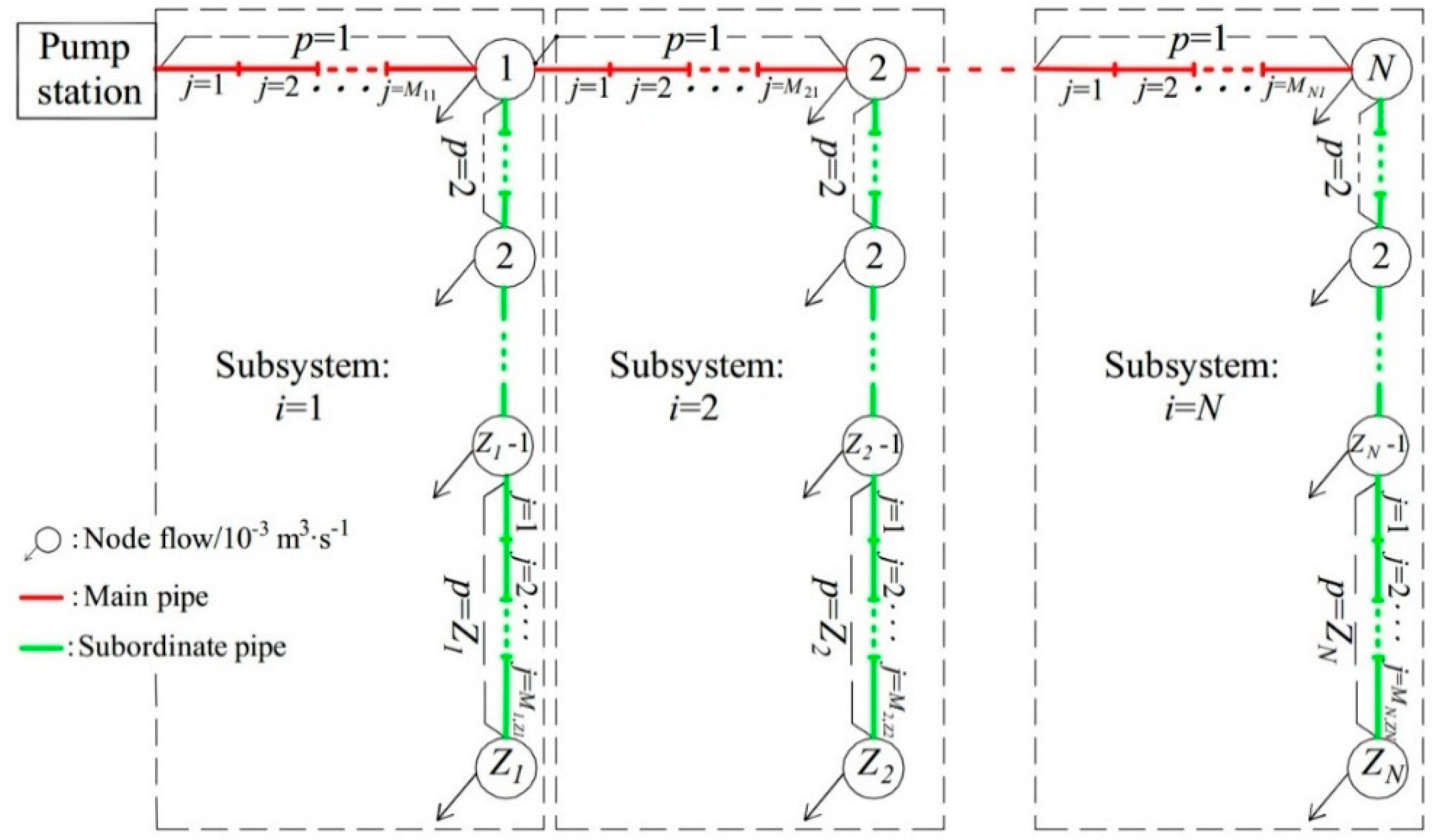
2. Mathematical Model

Commonly, a pressurized tree-type WDN consists of main, subordinate and branch pipes with multi-diameter pipes, and the pumping station is located at the water source [25,26]. The authors assume a pre-determined geographical structure of the pressurized tree-type WDN. The pipe material, flow and length are known. The generalization diagram is shown in Figure 1 along with a numbered scheme for pipes and nodes. The pressurized tree-type WDN can be divided into N subsystems (i = 1, 2, …, N, i is the subsystem number). Each subsystem is divided into Zi pipe segments (p = 1, 2, …, Zi, p is the pipe segment number in the i-th subsystem). Due to the differences of pipe materials and diameters, each pipe segment is further divided into Mip branch sections (j = 1, 2, …, Mip, j is the branch pipe number of the p-th pipe segment in the i-th subsystem).

2.1. Objective Function

The total investment cost of a WDN is the most common optimization objective, for which it is essential to determine the minimum spanning tree of the pipeline cost, based on the generalization diagram [5,27]. However, in addition to the investment cost, the operational cost of the pressurized pumping station is not negligible in pressurized tree-type WDNs. Thus, the equivalent annual cost (EAC) can better achieve the optimization objective of this network. EAC is the sum of annual investment, depreciation, maintenance cost and pump operational cost [16,28]. The minimum EAC (W) can be estimated by considering pump head and pipe diameter as double decision variables as follows:
W = min (A·FI + B·FI + Y)
where A is the reimbursement coefficient of the investment (RMB); B is the factor of annual depreciation and maintenance (%); FI is the investment cost (RMB). With the given base structure of the network, FI can be given as:
F I = i = 1 N p = 1 Z i j = 1 M i p ( a + b D i p j χ ) l i p j
where a, b and χ are the cost coefficients of the ipj-th pipe, which depends on pipe materials and local economic factors; lipj is the length of the ipj-th pipe (m); Dipj is the decision variable representing the diameter of the ipj-th pipe (m).
Y is the annual operational cost of pumps (RMB) and can be defined as:
Y = P Q p h p
where P is the power cost coefficient (RMB/(m3/s·m·a)); Qp is the pumping station flow (m3/s); hp is the decision variable representing the pump head (m).
By substituting Equations (2) and (3) into Equation (1), the objective function can be written as:
W = min [ ( A + B ) i = 1 N p = 1 Z i j = 1 M i p ( a + b D i p j χ ) l i p j + P Q P h P ]

2.2. Constraint Conditions
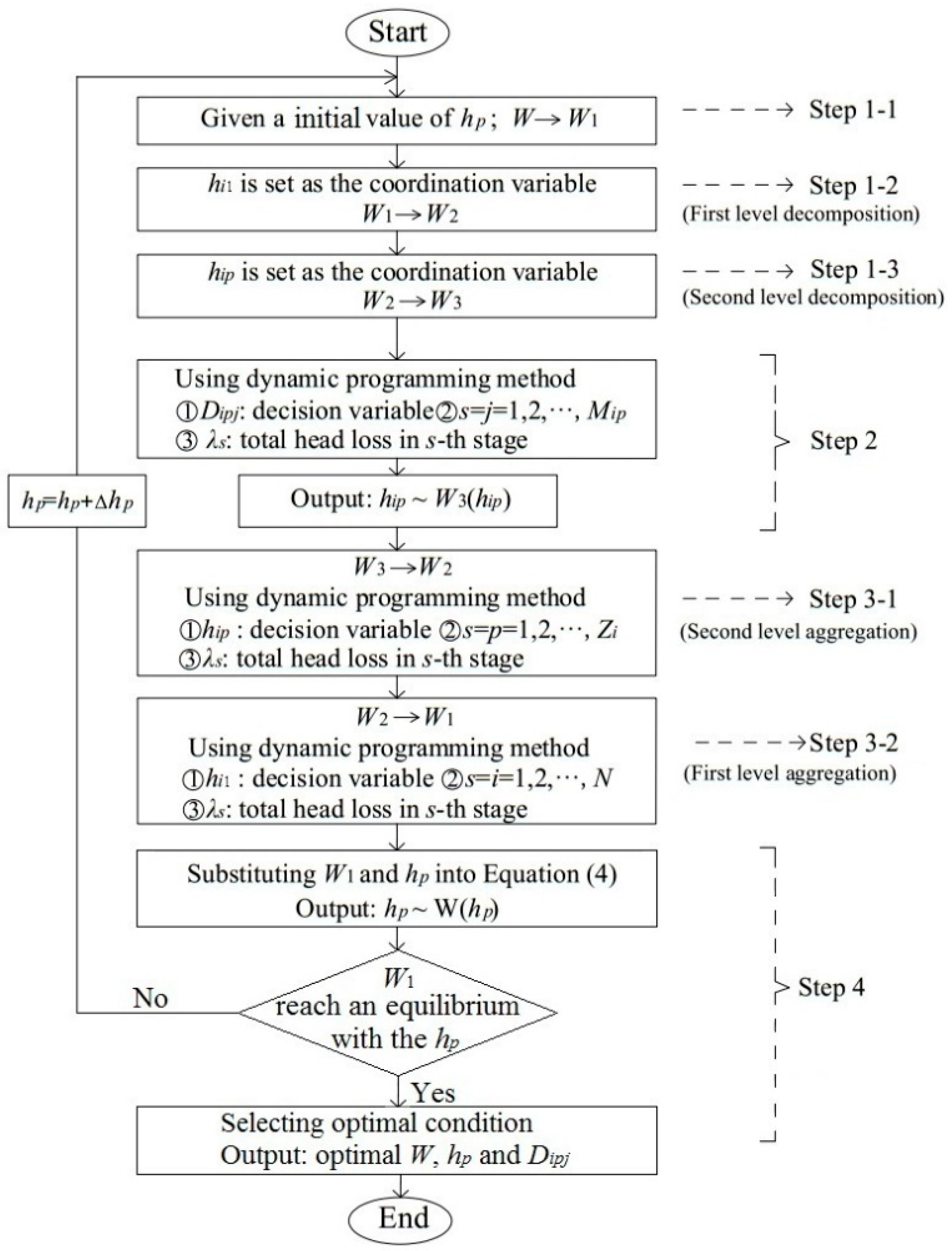
The pipe head loss and flow velocity should be considered as constraint conditions [1,29]. In the optimization process, the nonlinear objective function is subjected to the following constraints:
The total head loss of the main pipe (Hmain), the total head loss of the i-th subsystem (Hsub,i) and the head loss of each main or subordinate pipe in the subsystem (Hsub,ip) should be equal to or lower than the maximum allowable head loss of their corresponding pipeline.
H m a i n H t
H s u b , i H t , i
H s u b , i p H t , i p
where Hmain (m), Hsub,i (m) and Hsub,ip (m) are calculated by using the Hazen-Williams formula: H = klQ1.852/D4.87 (k is the roughness depending on the pipe material; Q is the pipe flow (m3/s)); Ht (m) is the maximum allowable head loss of the main pipe, which can be calculated by: Ht = hp + E0EN; E0 is the water source elevation (m); EN is the elevation of minimum service water head at Node N (m); Ht,i (m) is the maximum allowable head loss of the i-th subsystem; Hip (m) is the maximum allowable head loss of each main or subordinate pipe in i-th subsystem; Ht,i and Hip are the elevation difference between the water head at the beginning and the minimum service water head at the end of corresponding pipeline, which are dynamic changes with the different head distribution of main pipe.
The velocity of the ipj-th pipe (vipj) should be within the allowable maximum velocity (vmax) and minimum velocity (vmin) range depending on pipe materials as follows:
v m i n v i p j v m a x
Nonnegative constraints were given by:
D i p j 0 ;   h p 0

3. Model Solution

The model above is a complex nonlinear optimization problem with pump head and a large number of diameter variables needing to optimize synchronously. The improved decomposition–dynamic programming aggregation (DDPA) algorithm is employed to solve the sequential decision problems in large-scale network systems. The basic strategy of the DDPA algorithm in previous studies is [30,31]: (1) Decomposing the complex large system into subsystems and determining coordination variables; (2) using one-dimensional dynamic programming to optimize each subsystem separately; (3) establishing an aggregation model based on the relationship between the associated variables and the optimal value of each subsystem; (4) obtaining the global optimal solution of the associated variable and the corresponding optimal value. In this way, the DDPA algorithm can convert large system problems into multi-stage processes to cope with the curse of dimensionality and achieve improved feasible solutions. Compared with traditional decomposition/aggregation (DA) algorithms, the calculation precision can be significantly improved with the computational effort reduced. This is due to the fact that the DDPA algorithm leads to the formulation of dynamic programming programs in the aggregation processes instead of regression equations [32,33].
The optimization model in this work was constructed to find the best pump head and optimal diameters that minimized the EAC of pressurized tree-type WDAs. Thus, the DDPA algorithm process should to be improved to meet the optimization model. The improved algorithm process is summarized in Figure 2, and the main steps are detailed as follows:
Step 1: Converting double decision variables problem into single decision variable problem and decomposing the network system.
(1) Given a value of pump head.
After determining a pump head of pumping station (hp), Y is constant here based on Equation (3). The optimization function of double decision variables (W) can be converted to solve the problem of minimum annual investment, depreciation and maintenance cost (W1) with a single decision variable. This is different from the previous DDPA algorithm [30,31].
W 1 = ( A + B ) min F I = ( A + B ) min i = 1 N p = 1 Z i j = 1 M i p ( a + b D i p j χ ) l i p j
(2) First level decomposition.
According to the structure of WDNs (Figure 1), W1 can be decomposed into N subsystem models. The head loss of main pipe (hi1) is set as the coordination variable. The objective function of the i-th subsystem (i = 1,2, …, N) is expressed as:
W 2 = ( A + B ) min p = 1 Z i j = 1 M i p ( a + b D p j χ ) l p j
where W2 is the minimum annual investment, depreciation and maintenance cost of the i-th subsystem; Dpj is the decision variable representing the pj-th pipe diameter in the i-th subsystem.
To address the i-th subsystem, the constraints are similar to those in Equations (6)–(9). Besides, the head loss of the i-th main pipe (Hmain,i) should be less than or equal to hi1 and the maximum allowable head loss of the i-th pipe (Hi1).
H m a i n , i min { h i 1 , H i 1 }
(3) Second level decomposition.
Due to the difference in the combination of main and subordinate pipe sections, the objective model above (Equations (11) and (12)) is still an unsolvable problem. Thus, it is necessary to conduct the second level decomposition. W2 is further decomposed into Zi single-unit models. The head loss of the main and subordinate pipe in the i-th subsystem (hip) is set as the coordination variable. The objective function is expressed as Equation (13):
W 3 = ( A + B ) min j = 1 M i p ( a j + b j D j χ j ) l j
where W3 is the minimum annual investment, depreciation and maintenance cost of the p-th pipe segment in the i-th subsystem; Dj is the decision variable representing the j-th pipe diameter in the p-th single-unit models (p = 1, 2, …, Zi).
The velocity and nonnegative constraints are similar to those in Equations (8) and (9). Besides, the head loss of each main or subordinate pipe segment (Hsub,ip) should be less than or equal to hip and the maximum allowable head loss (Ht,ip).
H s u b , i p min { h i p , H t , i p }
Step 2: Optimization of the second level decomposition model based on the one-dimensional dynamic programming method.
The single-unit subsystem (Equations (13) and (14)) is a classical problem that can be solved by the one-dimensional dynamic programming method. Stage variable is the number of each branch section (s = j = 1, 2, …, Mip). State variable (λs) is the total pipe head loss in the s-th stage. In each recurrence equation, λs is discretized by a certain step size within the feasible domain (0 ≤ λship). The state transfer equation can be deduced as: λs−1 = λshs (hs is the head loss of the s-th branch section). For details of the calculation process, refer to Howard (1966) [34]. In this way, a W3 and the corresponding hip can be calculated in a single working condition of the single-unit subsystem. In order to obtain all working conditions of each single-unit subsystem, we dispersed the Ht,ip from 0 to the maximum with a certain step size. A series of W3 and hip can be determined in different values of discrete Ht,ip by reusing the one-dimensional dynamic programming method.
Step 3: Establishing and optimizing large system aggregation models.
(1) Second level aggregation.
According to the relationship between hip and W3 (hip) in single-unit subsystems from Step 2, each subsystem model (Equations (11) and (12)) can be aggregated by corresponding single-unit subsystems, considering hip as the decision variable. Thus, the W2 and head loss constraint can be written as follows:
W 2 = ( A + B ) min p = 1 Z i W 3 ( h i p )
p = 1 Z i h i p H t , i
The second level aggregation models above can also be solved by one-dimensional dynamic programming aggregation. Stage variable is the number of each main and subordinate pipe in the i-th subsystem (s = p = 1, 2, …, Zi). λs is the total pipe head loss in the s-th stage. A W2 of the subsystem and the corresponding hi can be calculated. Similarly, in order to obtain all working conditions of each subsystem, Ht,i is discretized with a certain step size. A series of relationships between hi1 and W2 (hi1) can be obtained based on the one-dimensional dynamic programming method.
(2) First level aggregation.
Then, the optimization function W1 can be converted by considering hi1 as the decision variable.
W 1 = ( A + B ) min i = 1 N W 2 ( h i 1 )
The corresponding constraint is expressed as:
i = 1 N h i 1 H t
In this case, stage variable is the number of main pipe (s = i = 1, 2, …, N); λs is the total head loss of main pipe in the s-th stage; W1 is determined in the given hp by using one-dimensional dynamic programming aggregation again. Then, the optimal W in this given hp can be calculated by substituting W1 and hp into Equation (4).
Step 4: Obtaining the global optimal solution.
The value of hp is discretized at a certain step size in the feasible region. By repeating Steps 1 to 3, a series of W can be obtained under corresponding values of hp. Among these optimization schemes, the minimum W is the optimal solution. Then, the corresponding optimized hp and the optimal distribution value of Dipj can be determined according to the model optimization results.

4. Application and Optimization Results

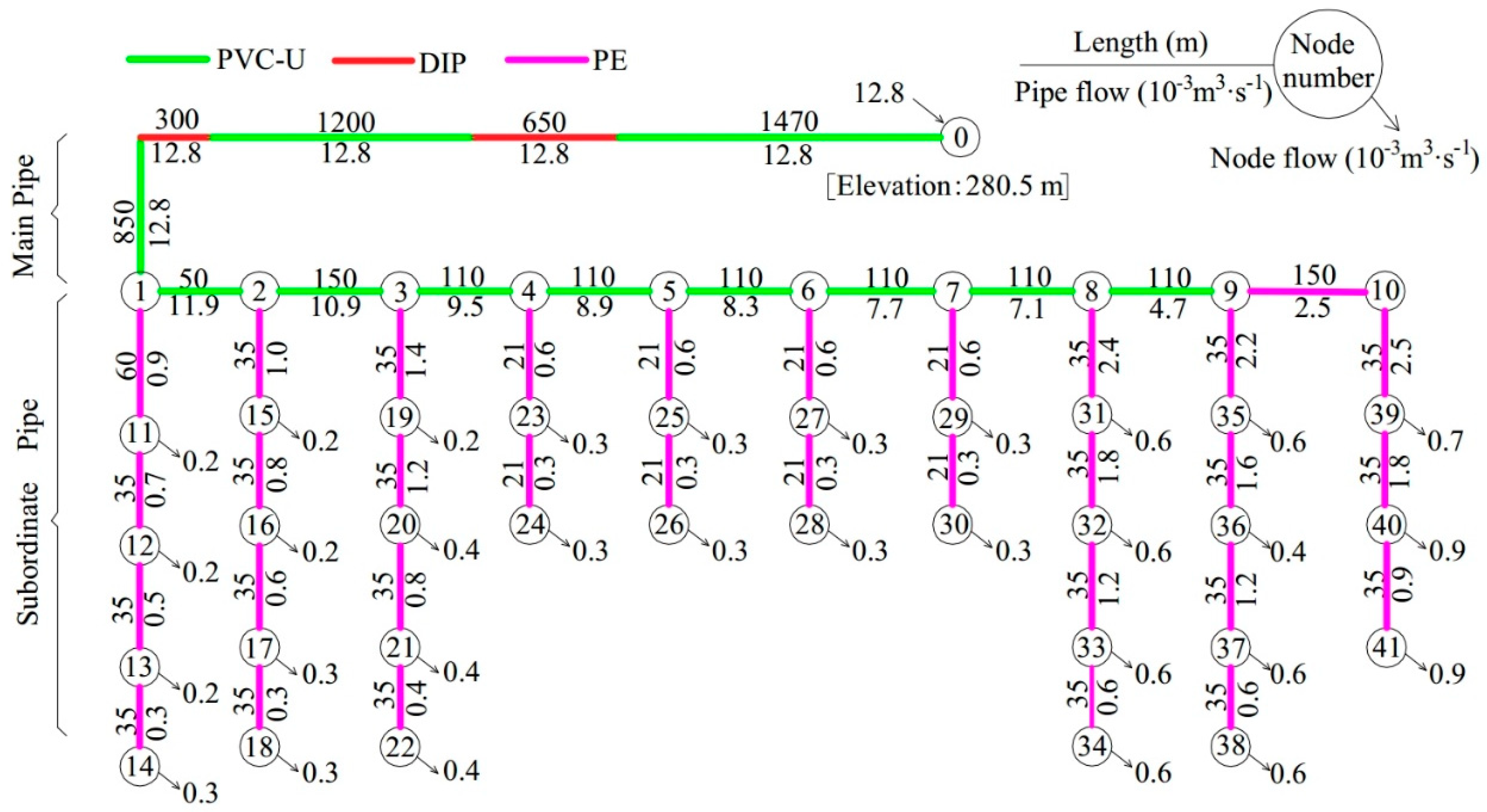
4.1. General Situation for a Pressurized Tree-Type WDN

A pressurized tree-type WDN was selected as a case study in rural area of Xinjiang Uygur Autonomous Region, China. The pipe flow, materials, lengths, nodal demands and elevation are detailed in (Figure 3). This WDN consisted of one source node, 41 demand nodes and 45 pipes. It was a pressurized tree-type WDN from a single fixed head source and was designed to satisfy the consumer demands at the required pressures. Due to the different terrain and external loads along the pipeline, the main pipe was composed of unplasticized poly (vinyl chloride) pipes (PVC-U) (4380 m), ductile iron pipes (DIP) (950 m) and polyethylene pipes (PE) (150 m). The subordinate pipe was composed of PE (998 m). The elevation of source node (E0) was 280.5 m. The minimum service water head at Node 10 and the end of each subsystem (Nodes 14, 18, 22, 24, 28, 30, 34, 38 and 41) were 20.0 m and 12.0 m, respectively. The demand nodes’ elevations (Nodes 1–41) were basically similar and exceeded the source (Node 0) by 48.6 m.

4.2. Solution Procedures

The 45 pipe diameters and pump head (hp) need to be optimized in this network with a total of 52 constraints of head loss. Firstly, the value range of diameters in each pipe can be determined by Q = π·v·D2/4, according to the velocity constraint of each pipe (v, Equation (8)) and the corresponding pipe flow (Q, shown in Figure 3). Then, available commercial diameters of each pipe can be selected, and the corresponding unit costs are listed in Table 1. Based on the relationship between diameters and unit costs, the cost coefficients of a, b and χ can be calculated by using the least square method (R2 > 0.98). For PVC-U, a = 4.1, b = 3529.3 and χ = 2.1; For DIP, a = 3.8, b = 4252.1 and χ = 2.1; for PE, a = −8.1, b = 379.3 and χ = 1.0.
The initial value of hp was set as 96.00 m, and increased with a certain step length (△hp = 0.05 m). For each network with certain hp, the corresponding minimum EAC (W, Equation (1)) could be solved by using the improved DDPA algorithm above. Thus, the relationship curve between hp and W could be confirmed (shown in (Figure 4)). The optimal W was 64,085 RMB and the best hp was 97.15 m. In this optimal layout (hp = 97.15 m), the optimal diameter of each branch section could be found by checking the model. The details of the optimal diameters are shown in Table 2.

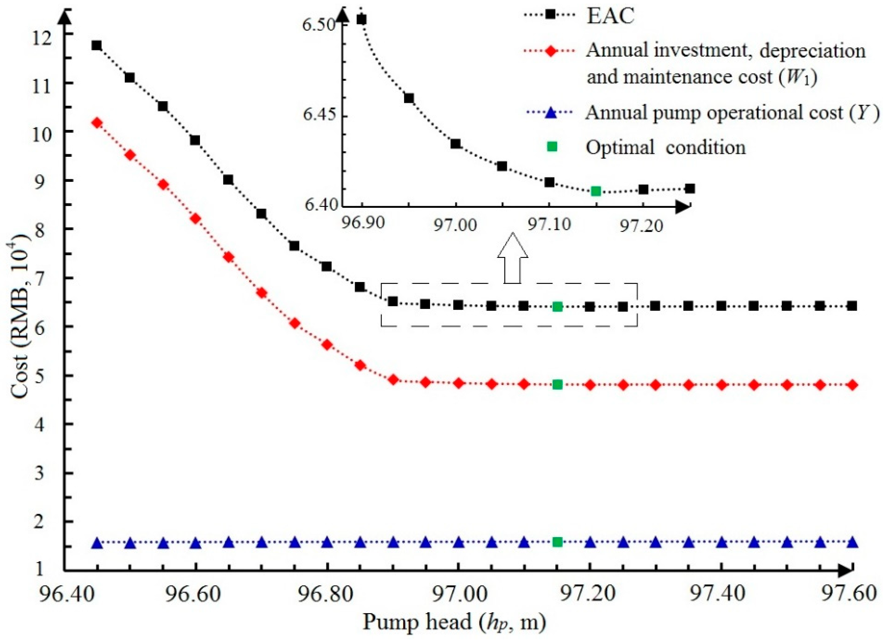
4.3. Optimization Results Analysis

As shown in Figure 4, the annual investment, depreciation and maintenance cost (W1) decreased sharply from 101,708 to 49,122 RMB (hp = 96.45–96.90 m). This was due to the optimization of the main pipe diameters, which accounted for up to 85% of total W1. When the hp value changed from 96.90 to 97.10 m, W1 decreased slowly and approached an equilibrium. W1 remained a constant of 48,134 RMB (hp ≥ 97.15 m), as the pipe diameters approached their minimum diameters. Besides, the pump operational cost (Y = PQphp) increased slowly with the increase of hp. As EAC is the sum of W1 and Y, the minimum EAC (W) was 64,085 RMB and the optimal hp was 97.15 m.
In contrast, the actual layout of this network is presented in Table 2 and was designed under the guidance of the Code for Urban Water Supply Engineering Planning (GB 50282-2016). The W1 was 62,026 RMB and exceeded by 22.5% the optimal layout, due to the actual diameters, which were significantly larger than optimal diameters (Table 2). The Y of the actual layout was 13,526 RMB, which was 17.9% less than the optimal layout. The lower hp (83.4 m) and larger pipe diameter reduced the head loss. It is worth noting that the head loss of the most disadvantaged pipeline route (Nodes 0–41) was 33.8 m (actual layout) and 58.6 m (optimal layout). Overall, the EAC was an intrinsic trade-off between W1 and Y. The EAC was 75,552 RMB in actual layout, which was 15.2% more than optimal layout. The results showed that the improved DDPA algorithm could find the minimum value under the joint action of investment and pump operational cost in a pressurized tree-type WDN.

5. Conclusions

In this paper, a large-scale WDN of pressurized tree-type was preset to establish a discrete nonlinear model for minimizing the EAC. The pump head and pipe diameters were decision variables. The head loss and flow velocity were the constraint conditions. An improved DDPA algorithm was proposed to solve the formulated optimization model.
The algorithm was applied to a real-world, large-scale regional WDN in China. The optimal scheme of EAC was determined by reducing W1 and increasing Y, and was reduced by 15.2% compared to the actual layout. The least-cost combination of pipe diameters and pump head could also be found. The results demonstrated the applicability of the proposed algorithm in decision-making for pressurized tree-type WDNs. We believe that, for better application of the large-scale WDN, additional reliability and resilience of the network should be considered in further studies.

Author Contributions

In this research work, H.C. and J.C. were involved in the conceptualization, methodology, software and validation under the joint supervision of L.W. and Y.W.; W.W. and Y.G. were involved in formal analysis and methodology; Y.C. wrote the paper. All authors approved the final version of the paper.

Funding

This work was supported by the National Key R&D Program of China (Grant No. 2017YFC0403205), the National Natural Science Foundation of China (Grant No. 51809226), the China Postdoctoral Science Foundation funded project (Grant No. 2018M632390), the natural Science Foundation of the Jiangsu Higher Education Institutions of China (Grant No. 18KJB610022 and 18KJD570001) and the Xuzhou Science and Technology Innovation project (Grant No. KC16SG283).

Conflicts of Interest

The authors declare no conflicts of interest.

References

  1. Bello, O.; Abu-Mahfouz, A.M.; Hamam, Y.; Page, P.R.; Adedeji, K.B.; Piller, O. Solving Management Problems in Water Distribution Networks: A Survey of Approaches and Mathematical Models. Water 2019, 11, 562. [Google Scholar] [CrossRef]
  2. Mala-Jetmarova, H.; Sultanova, N.; Savic, D. Lost in Optimisation of Water Distribution Systems? A Literature Review of System Design. Water 2018, 10, 307. [Google Scholar] [CrossRef]
  3. Makaremi, Y.; Haghighi, A.; Ghafouri, H.R. Optimization of Pump Scheduling Program in Water Supply Systems Using a Self-Adaptive NSGA-II; a Review of Theory to Real Application. Water Resour. Manag. 2017, 31, 1283–1304. [Google Scholar] [CrossRef]
  4. Coelho, B.; Andrade-Campos, A. Efficiency achievement in water supply systems-A review. Renew. Sustain. Energy Rev. 2014, 30, 59–84. [Google Scholar] [CrossRef]
  5. Zhao, W.Q.; Beach, T.H.; Rezgui, Y. Optimization of Potable Water Distribution and Wastewater Collection Networks: A Systematic Review and Future Research Directions. IEEE Trans. Syst. Man Cybern. Syst. 2016, 46, 659–681. [Google Scholar] [CrossRef]
  6. Vilanova, M.R.N.; Balestieri, J.A.P. Energy and hydraulic efficiency in conventional water supply systems. Renew. Sustain. Energy Rev. 2014, 30, 701–714. [Google Scholar] [CrossRef]
  7. Cisty, M. Hybrid Genetic Algorithm and Linear Programming Method for Least-Cost Design of Water Distribution Systems. Water Resour. Manag. 2010, 24, 1–24. [Google Scholar] [CrossRef]
  8. Shiono, N.; Suzuki, H.; Saruwatari, Y. A dynamic programming approach for the pipe network layout problem. Eur. J. Oper. Res. 2019, 277, 52–61. [Google Scholar] [CrossRef]
  9. Meirelles, G.; Brentan, B.; Izquierdo, J.; Ramos, H.; Luvizotto, E. Trunk Network Rehabilitation for Resilience Improvement and Energy Recovery in Water Distribution Networks. Water 2018, 10, 693. [Google Scholar] [CrossRef]
  10. Cherchi, C.; Badruzzaman, M.; Oppenheimer, J.; Bros, C.M.; Jacangelo, J.G. Energy and water quality management systems for water utility’s operations: A review. J. Environ. Manag. 2015, 153, 108–120. [Google Scholar] [CrossRef]
  11. Martinez-Bahena, B.; Cruz-Chavez, M.A.; Avila-Melgar, E.Y.; Cruz-Rosales, M.H.; Rivera-Lopez, R. Using a Genetic Algorithm with a Mathematical Programming Solver to Optimize a Real Water Distribution System. Water 2018, 10, 1318. [Google Scholar] [CrossRef]
  12. D’Ambrosio, C.; Lodi, A.; Wiese, S.; Bragalli, C. Mathematical programming techniques in water network optimization. Eur. J. Oper. Res. 2015, 243, 774–788. [Google Scholar] [CrossRef]
  13. De Corte, A.; Sörensen, K. Optimisation of gravity-fed water distribution network design: A critical review. Eur. J. Oper. Res. 2013, 228, 1–10. [Google Scholar] [CrossRef]
  14. De Corte, A.; Sörensen, K. An Iterated Local Search Algorithm for Multi-Period Water Distribution Network Design Optimization. Water 2016, 8, 359. [Google Scholar] [CrossRef]
  15. Azoumah, Y.; Bieupoude, P.; Neveu, P. Optimal design of tree-shaped water distribution network using constructal approach: T-shaped and Y-shaped architectures optimization and comparison. Int. Commun. Heat Mass Transf. 2012, 39, 182–189. [Google Scholar] [CrossRef]
  16. Dobersek, D.; Goricanec, D. Optimisation of tree path pipe network with nonlinear optimisation method. Appl. Therm. Eng. 2009, 29, 1584–1591. [Google Scholar] [CrossRef] [Green Version]
  17. Perelman, L.S.; Amin, S. Control of tree water networks: A geometric programming approach. Water Resour. Res. 2015, 51, 8409–8430. [Google Scholar] [CrossRef]
  18. Sangiorgio, M.; Guariso, G. NN-Based Implicit Stochastic Optimization of Multi-Reservoir Systems Management. Water 2018, 10, 303. [Google Scholar] [CrossRef]
  19. Castelletti, A.; Galelli, S.; Restelli, M.; Soncini-Sessa, R. Tree-based reinforcement learning for optimal water reservoir operation. Water Resour. Res. 2010, 46, 1–19. [Google Scholar] [CrossRef]
  20. Abdullah, M.A.; Ab Rashid, M.F.F.; Ghazalli, Z. Optimization of Assembly Sequence Planning Using Soft Computing Approaches: A Review. Arch. Comput. Methods Eng. 2019, 26, 461–474. [Google Scholar] [CrossRef]
  21. Batchabani, E.; Fuamba, M. Optimal Tank Design in Water Distribution Networks: Review of Literature and Perspectives. J. Water Resour. Plan. Manag. 2014, 140, 136–145. [Google Scholar] [CrossRef]
  22. Lamaddalena, N.; Khadra, R.; Tlili, Y. Reliability-Based Pipe Size Computation of On-Demand Irrigation Systems. Water Resour. Manag. 2012, 26, 307–328. [Google Scholar] [CrossRef]
  23. Leon-Celi, C.; Iglesias-Rey, P.L.; Martinez-Solano, F.J.; Mora-Melia, D. A Methodology for the Optimization of Flow Rate Injection to Looped Water Distribution Networks through Multiple Pumping Stations. Water 2016, 8, 575. [Google Scholar] [CrossRef]
  24. Goncalves, G.M.; Gouveia, L.; Pato, M.V. An improved decomposition-based heuristic to design a water distribution network for an irrigation system. Ann. Oper. Res. 2014, 219, 141–167. [Google Scholar] [CrossRef]
  25. Basupi, I.; Kapelan, Z. Flexible Water Distribution System Design under Future Demand Uncertainty. J. Water Resour. Plan. Manag. 2015, 141, 1–14. [Google Scholar] [CrossRef]
  26. Farmani, R.; Abadia, R.; Savic, D. Optimum design and management of pressurized branched irrigation networks. J. Irrig. Drain. Eng. 2007, 133, 528–537. [Google Scholar] [CrossRef]
  27. Geem, Z.W. Multiobjective Optimization of Water Distribution Networks Using Fuzzy Theory and Harmony Search. Water 2015, 7, 3613–3625. [Google Scholar] [CrossRef]
  28. Zeng, J.; Han, J.; Zhang, G.Q. Diameter optimization of district heating and cooling piping network based on hourly load. Appl. Therm. Eng. 2016, 107, 750–757. [Google Scholar] [CrossRef]
  29. Price, E.; Ostfeld, A. Iterative Linearization Scheme for Convex Nonlinear Equations: Application to Optimal Operation of Water Distribution Systems. J. Water Resour. Plan. Manag. 2013, 139, 299–312. [Google Scholar] [CrossRef] [Green Version]
  30. Gong, Y.; Cheng, J.L. Optimization of Cascade Pumping Stations’ Operations Based on Head Decomposition-Dynamic Programming Aggregation Method Considering Water Level Requirements. J. Water Resour. Plan. Manag. 2018, 144, 04018034. [Google Scholar] [CrossRef]
  31. Gong, Y.; Cheng, J.L. Combinatorial Optimization Method for Operation of Pumping Station with Adjustable Blade and Variable Speed Based on Experimental Optimization of Subsystem. Adv. Mech. Eng. 2014, 2014, 283520. [Google Scholar] [CrossRef]
  32. Sadr, J.; Malhamé, R.P. Unreliable transfer lines: Decomposition/aggregation and optimization. Ann. Oper. Res. 2004, 125, 167–190. [Google Scholar] [CrossRef]
  33. Sadr, J.; Malhamé, R.P. Decomposition/aggregation-based dynamic programming optimization of partially homogeneous unreliable transfer lines. IEEE Trans. Autom. Control 2004, 49, 68–81. [Google Scholar] [CrossRef]
  34. Howard, R.A. Dynamic Programming. Manag. Sci. 1966, 12, 317–348. [Google Scholar] [CrossRef]
Figure 1. Generalization diagram of pressurized tree-type water distribution network (WDN).
Water 11 01391 g001
Figure 2. Flowchart of the proposed methodology.
Water 11 01391 g002
Figure 3. Generalization diagram of pressurized tree-type WDN in Xinjiang Uygur Autonomous Region, China (44°02′–45°23′ N, 79°53′–83°53′ E). PVC-U: Unplasticized poly (vinyl chloride) pipes; DIP: Ductile iron pipes; PE: Polyethylene pipes.
Water 11 01391 g003
Figure 4. Cost distribution at different pump heads (hp). EAC is the sum of annual investment, depreciation and maintenance cost (W1) and annual pump operational cost (Y). The optimal pump head (hp) of minimum EAC (W) was 97.15 m.
Water 11 01391 g004
Table 1. Available commercial pipe diameters and corresponding unit costs.
Diameter (m)Pipe Cost (RMB/m)
PVC-UDIPPE
0.025--2.2
0.032--4.5
0.040--7.1
0.0509.3-10.9
0.06314.516.217.1
0.07518.321.021.5
0.09025.629.230.1
0.11040.042.845.6
0.12550.555.960.3
0.14063.369.7-
0.16080.0092.0-
0.180101.2116.9-
0.200120.1160.2-
PVC-U: Unplasticized poly (vinyl chloride) pipes; DIP: Ductile iron pipes; PE: Polyethylene pipes. The corresponding unit costs depended on local economic factors.
Table 2. Optimization results of diameters in each branch section.
Number of Up and Down NodesMaterialsLength (m)Actual Diameter (m)Optimal Diameter (m)Number of Up and Down NodesMaterialsLength (m)Actual Diameter (m)Optimal Diameter (m)
0–1DIP+PE44700.1600.14021–22PE350.0250.025
1–2PVC-U500.1600.1404–23PE210.0320.025
2–3PVC-U1500.1400.14023–24PE210.0250.025
3–4PVC-U1100.1400.1105–25PE210.0320.025
4–5PVC-U1100.1250.11025–26PE210.0250.025
5–6PVC-U1100.1250.0906–27PE210.0320.025
6–7PVC-U1100.1250.09027–28PE210.0250.025
7–8PVC-U1100.1100.0907–29PE210.0320.025
8–9PVC-U1100.0750.07529–30PE210.0250.025
9–10PE1500.0630.0508–31PE350.0630.040
1–11PE600.0400.05031–32PE350.0500.040
11–12PE350.0400.03232–33PE350.0400.032
12–13PE350.0320.02533–34PE350.0320.025
13–14PE350.0250.0259–35PE350.0630.040
2–15PE350.0400.04035–36PE350.0500.040
15–16PE350.0400.04036–37PE350.0500.032
16–17PE350.0320.02537–38PE350.0320.025
17–18PE350.0250.02510–39PE350.0630.040
3–19PE350.0500.04039–40PE350.0500.040
19–20PE350.0500.04040–41PE350.0400.032
20–21PE350.0400.025
The actual layout was designed under the guidance of the Code for Urban Water Supply Engineering Planning (GB 50282-2016) with the economical flow velocity being 0.6–0.9 m/s.

