Article

River Model Calibration Based on Design of Experiments Theory. A Case Study: Meta River, Colombia

by
Guillermo J. Acuña
1,2,*,
Humberto Ávila
1 and
Fausto A. Canales
2
1
Department of Civil and Environmental Engineering, Instituto de Estudios Hidráulicos y Ambientales, Universidad del Norte, Km.5 Vía Puerto Colombia, Barranquilla 081007, Colombia
2
Department of Civil and Environmental, Universidad de la Costa, Calle 58 #55-66, Barranquilla 080002, Atlántico, Colombia
*
Author to whom correspondence should be addressed.
Water 2019, 11(7), 1382; https://doi.org/10.3390/w11071382
Submission received: 25 May 2019 / Revised: 25 June 2019 / Accepted: 29 June 2019 / Published: 5 July 2019

Abstract

:
Numerical models are important tools for analyzing and solving water resources problems; however, a model’s reliability heavily depends on its calibration. This paper presents a method based on Design of Experiments theory for calibrating numerical models of rivers by considering the interaction between different calibration parameters, identifying the most sensitive parameters and finding a value or a range of values for which the calibration parameters produces an adequate performance of the model in terms of accuracy. The method consists of a systematic process for assessing the qualitative and quantitative performance of a hydromorphological numeric model. A 75 km reach of the Meta River, in Colombia, was used as case study for validating the method. The modeling was conducted by using the software package MIKE-21C, a two-dimensional flow model. The calibration is assessed by means of an Overall Weighted Indicator, based on the coefficient of determination of the calibration parameters and within a range from 0 to 1. For the case study, the most significant calibration parameters were the sediment transport equation, the riverbed load factor and the suspended load factor. The optimal calibration produced an Overall Weighted Indicator equal to 0.857. The method can be applied to any type of morphological models.

1. Introduction

Numerical models have become an essential tool for researching and developing engineering solutions related to water resources problems [1]. Models enable complex underlying processes to be captured, and facilitate the analysis of interrelationships between variables in cases with limited data [2]. Modeling has major applications in fields such as hydrology, maritime and coastal studies [3,4], river hydraulics [5] and water quality [6].
Calibration is one of the most important activities within the modeling process, because the model’s credibility strongly depends on it [7]. The calibration process can be defined as adjusting the parameter values of a model in order to reproduce the real-world response within an accuracy range defined in the performance criteria (i.e., an acceptable level of adjustment between model and reality) [8,9]. The importance and impact of calibration on hydrological and hydraulics models has been assessed and confirmed by several authors [10,11,12,13].
According to Troy et al. [14], the process for calibrating the parameters required in a model can be classified in three categories: trial and error (manual) calibration, automatic optimization (generally through computer programs) and multistep automatic methods that take advantage of combining the strengths of manual and automatic calibration. The trial and error approaches provide more control to the modeler; however, manual adjustment may become too complex when the parameters to calibrate are numerous and correlated. The automatic optimization methods are based on three elements: an objective function, an optimization algorithm (that usually includes a set of constraints) and a convergence criterion. This type of calibration has been widely used in recent works related to hydrological and hydrodynamic modeling [10,11,15,16,17]. However, this type of calibration faces a numerical problem, the equifinality of the problem (i.e., that there might exist a set of different combinations of parameters for which the objective function returns the same value) [18]. It is also possible that the combination of values obtained in the calibration process is inconsistent with real world phenomena that the model tries to represent.
In general, river models consist of a combination of two or three of the following components: hydrodynamics, sediments and morphology. A river model calibration is usually focused on the hydrodynamic component, whose usual indicators are water surface levels and discharge under steady flow conditions [19]. The most common indicator for sedimentological calibration is the sediment transport rate [20,21]; however, this information is not always available and, furthermore, it may include high levels of uncertainty depending on the measuring or estimation techniques employed to obtain the data. Morphology calibration typically involves comparing field data on bathymetry as well as erosion and sediment transport rates, with results obtained from simulation. This type of calibration requires a set of parameters that allows sensitivity analysis to be performed on the simulated river form, in order to emulate field data conditions from an initial state to a final state [22]. Morphology calibration is complex and rarely performed, because topobathymetric data is usually unavailable [3]. Many numerical models are unable to effectively reproduce the physical processes related to the morphological evolution of the river channel [1], and understanding the relationship between the river channel morphology and erosion processes is the subject of many recent studies [23,24,25] aiming for a better understanding and forecasting of the river evolution.
Because of the difficulties commonly caused by the lack of sufficient and accurate data, as well as by poor model performance under certain conditions, the calibration of a hydromorphological model is usually complicated due to the interaction of its calibration parameters; consequently, the sequential adjustment of each parameter value might not be the most efficient calibrating method [26]. This may be even more relevant for rivers whose morphology is heavily affected by hydrological and sedimentological variations, because the slightest modification in the parameters of one of the three components (hydrodynamics, sediments or morphology) would possibly affect the adjustment of the other two. For example, a significant change in the river cross-section could influence flow velocities, water surface levels and shear stress, which in turn would impact on erosion and sediment transport processes. In such cases, a common calibration approach used by most consultants and researchers is to follow recommendations given by software developers and more experienced users. Nevertheless, these recommendations do not represent a structured method, and they are also hard to replicate when different conditions arise [27].
Within this context, the main contribution of this paper is to present a calibration method based on Design of Experiments (DOE) theory that allows: calibration of the model considering the interplay between the calibration parameters; identification of the most sensitive parameters within the calibration process; and determination of a value or a range of values for which the calibration parameters produce an adequate performance of the model in terms of accuracy. The method consists of a systematic process for assessing the qualitative and quantitative performance of a hydromorphological numeric model based on calibration parameters (riverbed level changes, velocity vectors, sediment transport rates, etc.).
The combination of sensitivity analysis and optimization techniques for a better model calibration has been described by van Waveren et al. [27] as a good modeling practices. The DOE approach presented in this paper incorporates these good practices while also allowing the modelers to get a better understanding of the effect of the calibration parameters on the adjustment indicators, which is a useful feature, especially for beginners in modelling. Using DOE to define the number of simulations might even reduce the computational times when compared to other heuristic approaches. Because it is based on DOE theory, the method aims at easy implementation and adjustment.
To validate the method, this paper presents a case study evaluating a 75 km-long reach of the Meta River, in Colombia. The modeling was conducted with MIKE-21C, a two-dimensional flow model which can analyze spatial and temporal variation in depth, bed level, velocity, and shear stress during extended time intervals [28]. Nevertheless, the method described in this paper can be coupled with similar hydromorphological models, many of them briefly described in [29].
The remainder of this paper has the following structure: Section 2 reports the set of parameters required for calibrating the model, and descriptions of the method and case study; Section 3 presents the model setup and the main results obtained by applying the method, followed by the corresponding discussion. Section 5 lists the main conclusions.

2. Materials and Methods

The method is summarized as follows: (i) definition of the model objective and possible simplifications; (ii) selection the calibration parameters and indicators used for hydrodynamic, sedimentologic and morphologic components; (iii) experiment design and calibration. After presenting the method, the river reach taken as the case study is described.

2.1. Modeling Objective and Simplifications

Some of the typical modeling purposes include: understanding the hydrodynamics, sediment transport or morphological development of a specific segment of a river; aiding in the design of ports, bridges and other hydraulic and navigation structures; assessing river restoration and management plans; analyzing aquatic ecosystems; etc. Defining the model objective is perhaps the most important step of the process. Once the objective is defined, and before calibrating the model, it is necessary to reduce the number of calibration parameters, in order to have a better understanding and control over the process. Depending on the spatiotemporal resolution of the simulations, the use that will be given to the results and the characteristics of the river in consideration, some parameters may become less significant. For example, the river hydrodynamic conditions may be such that the eddy viscosity calibration becomes unnecessary, possibly because it is not a sensitive parameter in the hydrodynamic adjustment process [30]. Another example is the existence of hydraulic structures or marginal protections providing riverbank erosion control [31], which in turn make the erosion rate parameter expendable.

2.2. Parameters Used as Hydrodynamic, Sedimentologic and Morphological Indicators

For every parameter considered during the calibration process, and in order to determine the goodness-of-fit of the model, a set of qualitative and quantitative indicators is defined for comparing measurements with the results from simulations. Qualitative indicators refer to variables difficult to compare at a specific time or place, or variables whose interpretation requires modeler experience. For this method, the goodness-of-fit of the calibration based on the quantitative indicators is measured by means of the coefficient of determination, also known as R-squared (R2), a statistical measure of how close the data fit the regression line, in this case, comparing whether the simulations match real-data. The method admits other statistical measures for goodness-of-fit, like the mean squared error (MSE) and the mean absolute error (MAE).
Based on suggestions by Matte et al. [32] and some common outputs from river models, a set of quantitative indicators were chosen to compose an Overall Weighted Indicator (OWI) for assessing calibration. The OWI is expressed as follows:
OWI = β1·WL + β2·QL+ β3·FD + β4·MP + β5·SST + β6·SBT + β7·ST + β8·BL + β9·BE,
where i = 1 n β i = 1 , and:
  • WL = coefficient of determination (R2) related to water level;
  • QL = coefficient of determination (R2) related to flow rate at control cross-sections;
  • FD = coefficient of determination (R2) related to flow distribution through island branches;
  • MP = coefficient of determination (R2) related to depth through the 2D domain;
  • SST = coefficient of determination (R2) related to suspended-load sediment transport;
  • SBT = coefficient of determination (R2) related to bed load sediment transport;
  • ST = coefficient of determination (R2) related to total load sediment transport;
  • BL = coefficient of determination (R2) related to bed level through the 2D sector;
  • BE = coefficient of determination (R2) related to bank erosion rate.
The different values of βi correspond to the relative weight of each indicator on the OWI. These weights are usually chosen by consensus among the modeling team based on experience or based on the uncertainty related to the variables of each indicator. For beginners, the authors of this paper recommend using the same value for all βi, as explained by Chaves and Alipaz [33] based on Shannon’s principle of maximum entropy, which warrants that the probabilities of underestimating or overestimation the parameters would be the same, considering that the indicators and the parameters are random variables (with also random distributions).
It is worth mentioning that the OWI can be subdivided in terms of the components of the river model. Elements WL, QL, FD and MP are calibration parameters of the hydrodynamic component (OWIHD); SST, SBT and ST correspond to the sedimentological component (OWIST); while BL and BE are calibration parameters accounting for the morphological component (OWIMF).
The input parameters can be categorized into two types: those that can be determined from field measurements or obtained from literature or other reliable sources; and those that must be determined through calibration [8]. Table 1 shows some of the most common parameters required for modeling the hydrodynamic, sedimentological and morphological characteristics of a river. It is worth noticing that the calibration parameters listed in Table 1 emphasize the ones used by MIKE-21C, the computer model used as the main software tool in the present work.
Depending on the river characteristics or the chosen computational model (or numerical approach), the model might require more or less parameters. For instance, MIKE-21C was employed by de Villiers [35] for studying cohesive sediment transport in a shallow reservoir, including within this analysis some additional calibration parameters such as Critical Shear Stress for deposition (τde), Critical Shear Stress for erosion (τer), Erosion constant (E0) and Exponent of the erosion. Beck and Basson [36] assessed the hydraulic and sedimentological behavior of the Klein river estuary by means of MIKE-21C, including as calibration parameters: Hydrodynamic time step, Morphological time step, Flooding Depth, Drying depth, Median grain diameter, Mass density of sediment and Porosity, as well as the calibration parameters shown in Table 1. Therefore, if additional calibration parameters are required for a more accurate representation of the process, the authors of the present paper recommend to the reader to conduct a literature review in order to define the range of feasible values for each calibration parameter. For example, the critical shear stress for deposition (τde) and the critical shear stress for erosion (τer) are very variable parameters which have a great impact on sediment transport mechanisms, but some authors [25,35] have performed sensitivity analysis on these calibration parameters, that could be used as baseline for setting the range of feasible values.
In this paper, two types of visual analysis are defined: (i) a comparison between simulated and measured (ADCP) velocity vectors, and (ii) an assessment of the simulated and historical morphological behavior of the river. Low performance model setups are easily detected by visual analysis before any numerical analysis.

2.3. Experiment Design and Calibration

The aim of DOE is to maximize the information obtained from a minimum number of experiments. It also helps to determine which factors might affect the performance of the model [37].
Once the calibration parameters and goodness-of-fit statistics have been chosen, the proposed method considers a screening design of experiment (definitive screening type) that allows identifying which calibration parameters and interactions have a significant effect on the overall accuracy of the model [38,39]. For this screening design, authors propose using a 2k factorial type of experiment, which evaluates k calibration parameters, each of them having two alternatives or levels that must be defined according to its corresponding physical or numerical meaning [37,38,40]. In consequence, goodness-of-fit and OWI calculations must be performed for each possible combination defined in the 2k experiment.
A second DOE aims at optimizing the calibration parameters whose effects (or the interactions with other parameter) were found as significant from the screening DOE. The present authors recommend a 3k type of experiment, that means, evaluating these parameters for at least three different representative levels from their previously defined range of possible values [38]. However, following this recommendation depends on available resources. As in the previous DOE, goodness-of-fit and OWI calculations must be performed for each possible combination defined in the 3k experiment.
Depending on the results from the second DOE, it is possible to obtain a regression equation expressing the relationship between calibration parameters and the model response, as well as the corresponding goodness-of-fit statistic, allowing optimizing a specific component of the OWI. The calibration process proposed in this paper is represented, for a better understanding, in the flowchart shown in Figure 1.
The process begins with hydrodynamic calibration. For this component, the main calibration parameter is the roughness coefficient, since water depth and flow velocity are function of this parameter, and it also has influence on flow distribution between the islands. If the river topology presents a cross-section contraction or sudden change of direction, it is likely that the eddy viscosity coefficient will be another significant calibration parameter [41].
The present method is suitable for calibrating and modeling rivers with a significant relationship between hydrodynamics and morphology. Therefore, it is necessary to include the effect of river morphological changes when conducting hydrodynamic calibration. For the method explained in this document, it is proposed the use of a morphological seed or preliminary values for morphological calibration parameters. This would allow a preliminary calculation of the morphological component of the model, during hydrodynamics calibration. The selection of the morphological seed can be done through a conceptual analysis, by using reference values available in the literature or based on known values used in other sections of the same river or other rivers with similar characteristics.
Once the hydrodynamic calibration is complete, the process continues with the sedimentological and morphological calibration. As explained before, such calibration is performed by an experimental design which can be used to define the significant parameters, the interactions between them, and the range of values for the calibrating parameters that provide a good fit between the results of the model and the observed data. When assessing the calibration of the morphological (OWIMF) and sedimentological (OWIST) components of the Overall Weighted Indicator, it is important to maintain the calibration of the hydrodynamic component and its corresponding parameters.
It is worth mentioning that the method can be used for unidimensional or multidimensional models (2D or 3D). A greater quantity of calibration parameters and indicators increases the required computational processing time, but it does not guarantee more accuracy.

2.4. Case Study: A Reach of the Meta River, Colombia

The Meta River is one of the major tributaries of the Orinoco river. The methods and results presented in this paper were produced from a project called “Update of studies and designs for navigation between Cabuyaro (K804) and Puerto Carreño (K0)” [42], conducted by Universidad del Norte (UNINORTE) in 2013, for the Colombian National Roads Institute (INVIAS) and the Colombian Ministry of Transport. From the field measurements made, the length of the Meta River was calculated as 1002 km, from its source near the town of Guamal, in the Meta Department, to its mouth in the Orinoco river. The Meta River watershed is approximately 99,500 km2 in area.
Recovering and improving navigability in Colombian rivers has been one of the main goals of the Colombian government over the last years [43]. For this reason, the aforementioned project was commissioned in order to analyze and model the Meta River, aiming at identifying the actions required to improve its navigability conditions.
The main data for this study consists of water depth, velocity and flow rate measurements, taken at the Orinoco river mouth (K0) and near the town of Cabuyaro (K796). The measurements were taken in two field campaigns that occurred between August 2012 and January 2013. Besides these on-site measurements, hydrological records from the Institute for Hydrology, Meteorology and Environmental Studies of Colombia (IDEAM) and Landsat (NASA) satellite imagery were other sources of information used for this case study.
The navigable channel of the Meta River is very unstable, and the flow and water depth variations through the year are significant and often abrupt, which causes some boats to become stranded. At the same time, the river presents high erosion and sedimentation rates [44]. From historical records between 1983 and 2010 at the IDEAM gauging station “Aceitico” (located 127 km upstream the mouth of the Orinoco), it was found that the average hydrograph presents maximum flow rates of around 10,323 m3/s, and minimum of around 755 m3/s. This ratio of 13.67 between maximum and minimum average indicates wide variability in flow rate in any given year. Furthermore, a unimodal trend was found in all hydrometric records; with high flow rates between May and August, and low flow rates between early December and late February.
Sedimentological measurements at the IDEAM stations in Puerto Texas (K669), Aguaverde (K360) and Aceitico (K127) show that sand and a small fraction of silt are the main materials transported by the river. The average grain size in the bed (D50-bed) is approximately 0.35 mm and the average grain size of the suspended particles (D50-susp) ranges between 0.057 and 0.17 mm. It is also worth noting that the flow rate in the river presents strong correlation with the sediment transport rate. According to the IDEAM records, this transport rate ranges between 419,680 and 4057 ton/day, based on data from Aceitico station for maximum and minimum average flow rates.
The results from the geomorphological studies carried out during the project showed that the Meta River morphology could be described as: 34% tabular, 26% sinuous / meandering, 24% straight, 10% braided and 6% anastomosed, based on satellite images from August and September 2012. Although the Meta River does not hold a particular morphological form, the selected satellite images, as well as aerial photographs taken between years 1986 and 2012 evidenced a high lateral and frontal mobility of the channel. From the analysis of the satellite images, it was also found that the floodplain of the river ranges from 3 to 9 km wide.
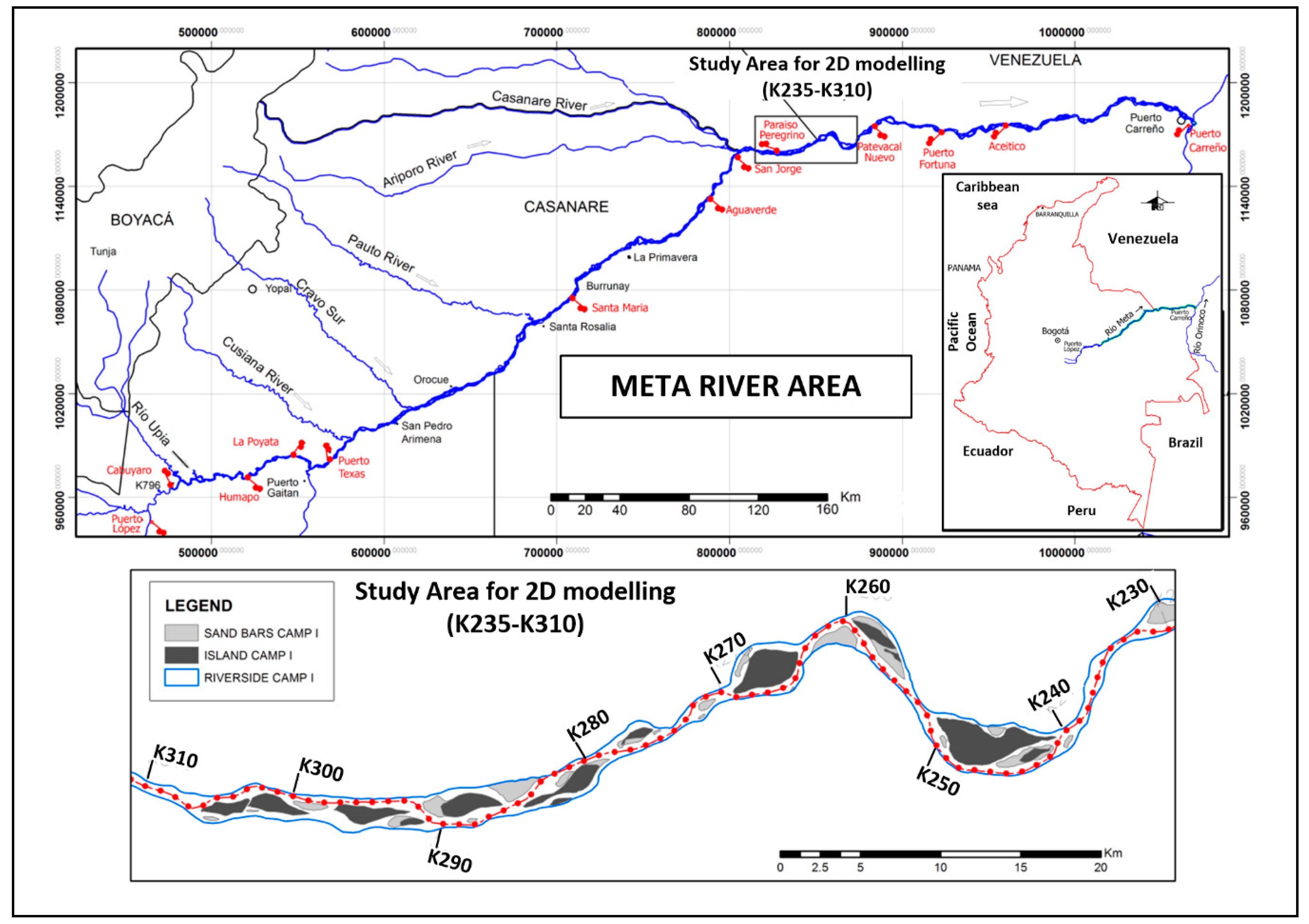
Based on the previous characterization and due to the technical and financial unfeasibility to model the whole river, a representative reach 75 km long was selected, between abscissas K235 (6°06′18.81″ N/69°12′55.04″ W) and K310 (6°02′50.38″ N/69°44′40.11″ W) (See Figure 2). The selection of this analysis section was based on:
  • Morphological Stability: this section presented a low riverbank variability between 1980 and 2012.
  • Hydraulic and sedimentological stability: this section is downstream of the last significant tributary of the Meta River, thus, variations in the hydraulic and sedimentological regime up to its mouth are not significant.
  • Morphological typology: presents a mix of braided, straight and sinuous reaches, indicating associated morphological response patterns along much of the river.

2.4.1. Indicators for the Meta River Model

As described in the previous section, the calibration process begins by selecting the available parameters that can be used to describe the river behavior. The rating curves for Meta River were obtained from the unidimensional model presented by UNINORTE [42], and this information was used as boundary conditions for hydrodynamic calibration.
The following comparable elements, based on the measurements obtained in the aforementioned study, were used as indicators for the calibration process of the Meta River model:
  • Adjustment of water level series (WL): Coefficient of determination (R2) between the hydrograph created from the water level series and the water level simulated by interpolation for the calibration period. The comparison point was set at the abscissa K310 corresponding to the upstream boundary condition.
  • Adjustment of flow distribution (FD): Coefficient of determination (R2) between the percentages of flow distribution through river branches around islands, measured on-site and those calculated by the 2D model.
  • Visual comparison of velocity vectors (Visual Indicator): A visual comparison was performed between the simulated velocity vectors and those recorded by the ADCP. It was considered that the average velocity value in the measured columns would occur close to 0.6 × H [45], where H is the height of the water column.
  • Adjustment of suspended sediment transport rate (SST): The IDEAM station “Aceitico” (K127) holds information regarding suspended sediment transport, estimated through regression models from data between 1996 and 2010. Based on the information available, the following equation was used in this work for estimating suspended sediment transport rate:
    QS = 0.0096·QL1.774,
    where QS is suspended sediment transport rate (ton/day) and QL is the river discharge (m3/s). To calculate R2, comparison was made between the QS values obtained by using discharge measurements and the ones calculated by using the results from the model.
  • Bed Level Adjustment (BL): The coefficient of determination (R2) was calculated between the mesh of riverbed levels created from the bathymetric surveys from field campaigns and those simulated by MIKE-21C.
  • Adequate morphological evolution (Qualitative Indicator): This visual indicator refers to the morphological evolution of the riverbed and riverbanks. The modeler shall verify if the morphologic changes through time are coherent with the numerical capabilities of the model, for example, no sudden and intense sedimentation or erosion phenomena occurred during the time span considered in the simulation.
For this case study, the OWI described in Equation (1) was divided into two components: The weighted indicator of hydrodynamic adjustment (OWIHD) and the weighted indicator of sedimentological and morphological adjustment (OWIST, MF). The βi coefficients were defined by the team of modelers participating of this project, based on agreed confidence levels for each variable measured during the field campaigns. Lower βi coefficients were assigned to variables with higher uncertainty levels.
OWIHD = 0.60 WL + 0.40 FD
OWIST, MF = 0.30 SST + 0.70 BL
By considering that both components have the same weight, the global OWI can be expressed as:
OWI = 0.30 WL + 0.20 FD + 0.15 SST + 0.35 BL

2.4.2. Parameters for Modeling the Meta River

For this case study, the modeling objective was to assess navigation capabilities in the Meta River. Based on this objective and the river characteristics, the modelers defined that:
  • For the river reach under consideration, the Chézy coefficient is used for quantifying bed resistance. In MIKE-21C, this value is estimated as a function of water depth, following the approach explained by Talmon [46]:
    Chézy = C·h0.17
    where Chézy is given in m1/2/s and h is the water depth in meters. Coefficient C (in m1/3/s) is the parameter to calibrate, and corresponds to the reciprocal of the Manning’s roughness coefficient [47], considered constant by the authors for this study. According to Talmon [46], this approach allows to incorporate small bathymetric irregularities (due to dunes, ripples, etc.) as bed resistance. The adequate calibration of the bed resistance directly impacts on the accuracy of the model to correctly estimate flow distribution and morphologic evolution. For example, if the resistance over a shallow region is too high, too much flow will be deflected and there will be a greater tendency towards developing sandbars [35].
  • According to the sedimentological information supplied by IDEAM, the median grain size in the riverbed (D50-bed) is 0.35 mm. Based on this grain size, García [48] suggests using Engelund-Hansen [49], Yang’s [50] and Van Rijn’s [51] equations for estimating sediment transport rates. From modeling studies carried out in 2003 Hidroconsultas LTDA [52] on the same river, it was observed that the sediment transport rates estimated by using Yang’s equation showed a good fit when compared to values from measurements. Based on this and aiming to reduce the number of variables in the study, the modelers decided to use only Yang’s and Van Rijn’s equations.
  • From the available imagery, it was found that riverbank variations in time intervals shorter than three years were not significant for the representative section. Islands were defined as covered with vegetation, which favors stability. The erosion rate at the riverbank and the corresponding coefficients were not considered as calibration parameters.
  • Due to absence of significant patterns and/or phenomena affecting the morphology, the helical flow coefficient HL was simplified to its default value of 1.00.
Based on the previous considerations, the calibration parameters for this case study can be summarized as:
  • Chézy Roughness coefficient as a function of depth; where C is the calibration parameter.
  • Sediment Transport Equation;
  • Riverbed Load Factor (Kb);
  • Suspended Load Factor (Ks);
  • Transverse Slope coefficient (TSC);
  • Transverse Slope power (TSP).

3. Results

This section describes the main results of the calibration process.

3.1. Hydrodynamic Calibration

To initiate the hydrodynamic calibration, it was necessary to define a sedimentological and morphological seed given as:
• Sediment Transport Equation: Van Rijn
• Riverbed Load Factor (Kb): 0.100
• Suspended Load Factor (Ks):0.300
• Transverse Slope coefficient (TSC):0.625
• Transverse Slope power (TSP): 0.500
The hydrodynamic calibration was focused on the adjustment of coefficient C in the roughness equation (Equation (6)). As seen in Table 2 and Table 3, three coefficient C values were evaluated for this purpose: 50, 55 and 60. As described in the previous section, their accuracy was assessed through the measured water levels and percentages of flow distribution through river branches as indicators. The best fit was obtained using C = 55, which results in an OWIHD = 0.9062, as shown in Table 3.
Once the hydrodynamic calibration has been conducted, the behavior of the velocity vectors is visually assessed, basically to verify if the model adequately represents this feature. An example of the model results for these visual comparisons is presented in Figure 3.

3.2. Screening Design—2k Experiment

The sedimentological and morphological components are calibrated using two consecutive experimental designs. The first design (2k) has the function of detecting the statistically significant factors. The parameters and levels at which the first design was evaluated are shown in Table 4.
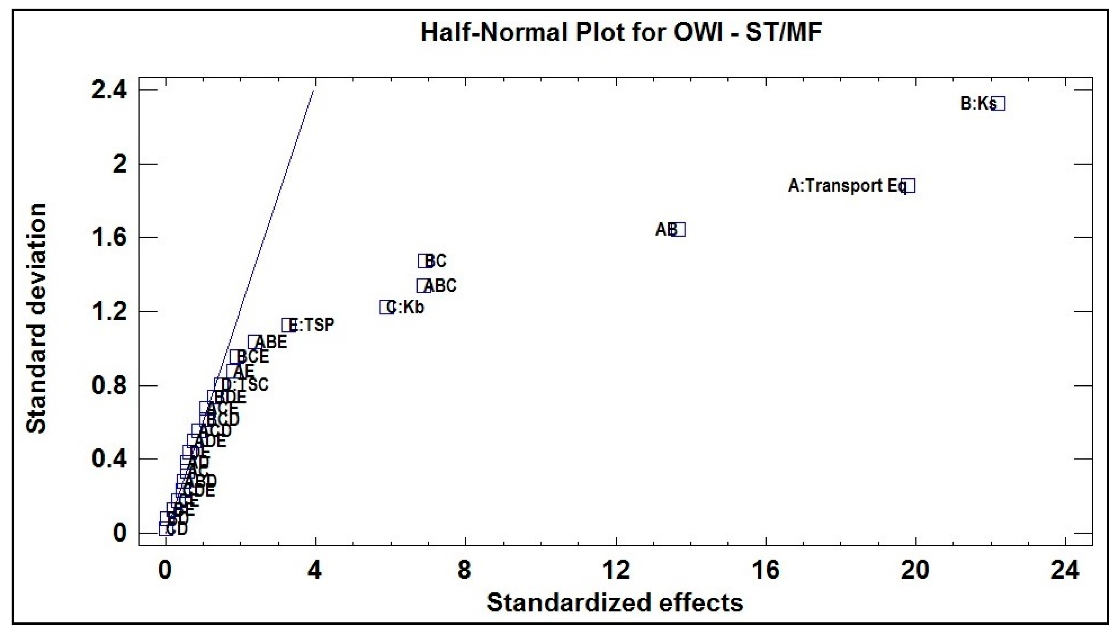
To determine which factors are statistically significant, it is necessary to perform an Analysis of Variance (ANOVA) using the results from simulation. As previously stated, this experiment does not include replicates, and consequently, the degrees of freedom of error within the ANOVA are few. This could induce to errors when estimating each parameter significance [38]. Therefore, before performing the ANOVA, it is necessary to identify which parameters have a significant effect on the model response and the probability of statistical noise, which might be interpreted as natural variability (error). To do so, a normality test was performed on the standardized effects of each parameter and its corresponding interactions, shown in Figure 4.
Once the most significant parameters and interactions have been identified, the ANOVA table is presented in Table 5. The R2 statistic indicates that the adjusted model explains 96.91% of the variability in OWIST, MF.
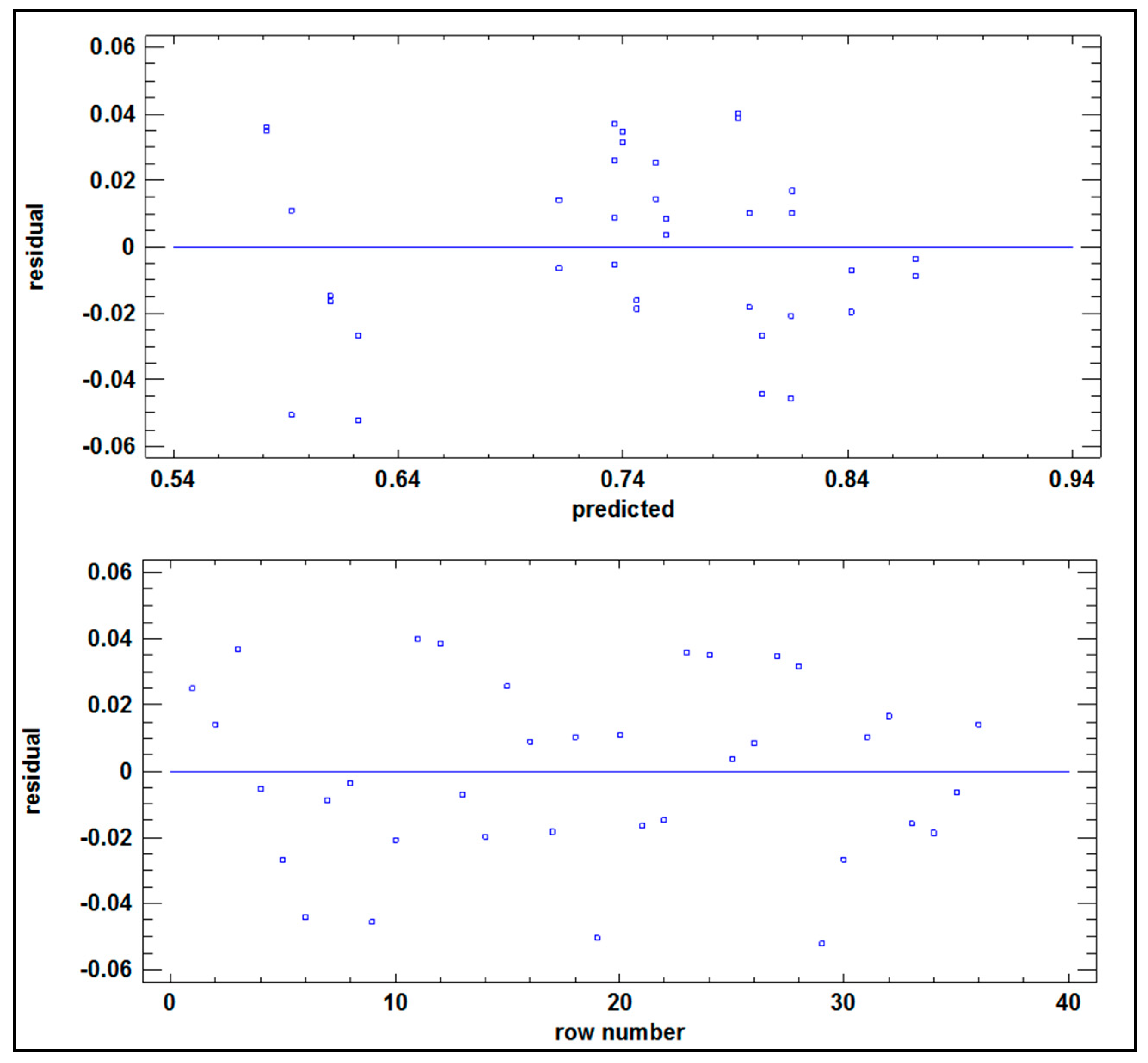
The statistical analysis for the 2k experiment shall be completed with the graphic verification of assumptions of Homoscedasticity, Normality and Independence. These charts are presented in Figure 5.

3.3. Fit Design—3k Experiment

This second DOE, of the 3k type, allows specifying the calibration value of the parameters. The parameters and levels at which the second design was evaluated are shown in Table 4. However, since some 2nd and 3rd order significant interactions were found at Table 5, they cannot be excluded from the experiment. Nevertheless, if all these interactions are considered, the necessary degrees of freedom in the residues will not be enough to perform the analysis of variance. Therefore, the modelers decided to vary the TSP as a replica generator, because it is one of the original main parameters whose effect was recognized as not significant at Figure 4. As previously defined at Table 4, the TSP was varied within the range from 0.5 to 1.
Based on the previous consideration, the parameters and levels at which this second design was evaluated are shown in Table 6, and the ANOVA results for this experiment are shown in Table 7, where all F-ratios are based on the mean square of residual error. The R2 statistic indicates that this fit model explains 97.69% of the variability in OWIST, MF. As in the 2k experiment, verification tests were performed for Homoscedasticity, Normality and Independence assumptions. Homoscedasticity and Independence charts are presented in Figure 6.
From the analysis of the individual behavior and interactions of the main parameters of this case study, the modelers observed that the higher OWIST, MF values were obtained when using the Van Rijn Transport equation.
Optimal calibration has as its objective to maximize OWIST, MF within the boundaries of the experimental region. From this, the best OWIST, MF result found was 0.864, associated with the following conditions: Van Rijn transport equation; Ks = 0.5; Kb = 0.1.
As described in the method section and summarized in Figure 1, once the morphological and sedimentological calibration has been performed and quantified by means of the OWIST, MF, the hydrodynamic component of OWI has to be checked in order to determine if its calibration remains valid.
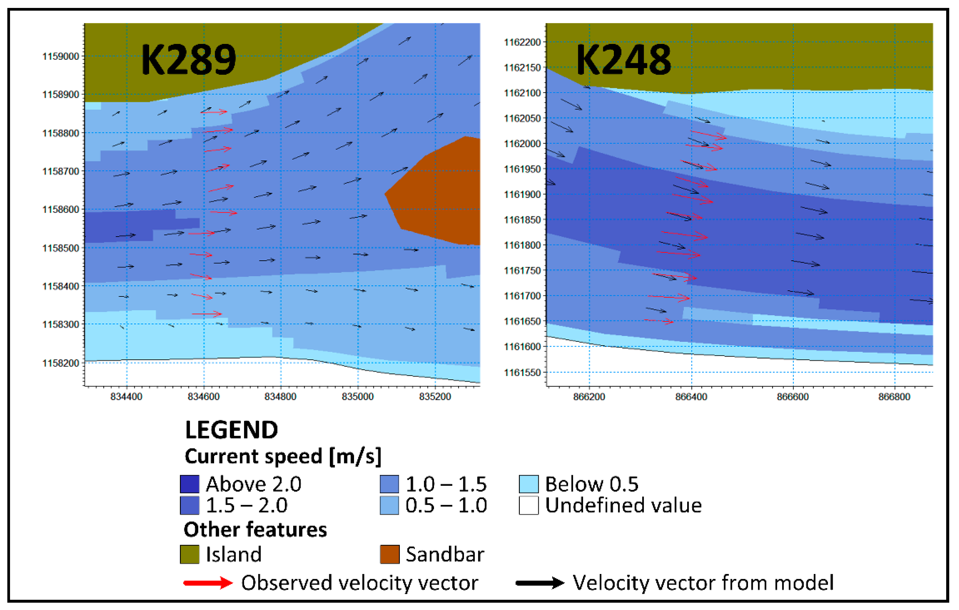
For this case study, the water level (WL) and flow distribution (FD) were calculated by the model using the conditions previously mentioned for optimizing OWIST, MF. An OWIHD of 0.90 was obtained from using those results. The qualitative calibration parameters related to velocity vectors and morphological evolution were also evaluated for this optimal case. For two sections of the river reach used as case study, Figure 7 displays the comparison between observed and modeled velocity vectors, where a good fit was observed both for magnitude and direction.
The morphological evolution was assessed and verified, with no significant instabilities or bathymetric changes found.

4. Discussion

4.1. Hydrodynamic Calibration

For the three different options of C, the error found between the simulated and observed values did not exceed 1.7%. Consequently, for this case study, the model sensitivity to this parameter is low, because in general, all the evaluated cases achieved an excellent adjustment when estimating water levels and flow distribution through river branches.
The visual inspection showed a good adjustment of the direction and magnitude of the average vectors extracted from the ADCP measurements with respect to the velocity vectors with respect to the simulated ones. The morphological behavior developed properly. There were no significant instability or abrupt changes in the bottom morphology of the river.

4.2. Screening Design—2k Experiment

Based on Figure 4, the most distant effects from the normal distribution trend were: B (Ks), A (Transport Equation), AB, BC, ABC, C (Kb). These were taken to perform the ANOVA analysis, allowing to dissect OWIST, MF variability and to evaluate the statistical significance of each effect by comparing its mean square against an estimate of the experimental error.
The results of the ANOVA Table concluded that the 6 evaluated effects include a P-value less than 0.05, indicating that they are significantly different from zero with a confidence level of 95.0%. From Figure 5 it can be observed that the graph of Residual vs. Predicted Values does not present any unusual structure. From the normality graph, it was observed that residues are correctly fitted to this type of statistical distribution. Finally, the graph of Residual vs. Order did not show any trend regarding the structure of execution; instead, the behavior of the Residual is erratic and dispersed.
From this screening experiment, it was found that just three of the five calibration parameters and only three interactions have significant effects on OWIST, MF. Based on this, only those three parameters were used for the second 3k type experiment design, or fit design.

4.3. Fit Design—3k Experiment

From this fit design experiment, the ANOVA summarized in Table 7 indicates that all factors and interactions considered are significant. With all P values smaller than 0.05, all the calibration parameters have a statistically significant effect on OWIST, MF, when considering a confidence level of 95%.
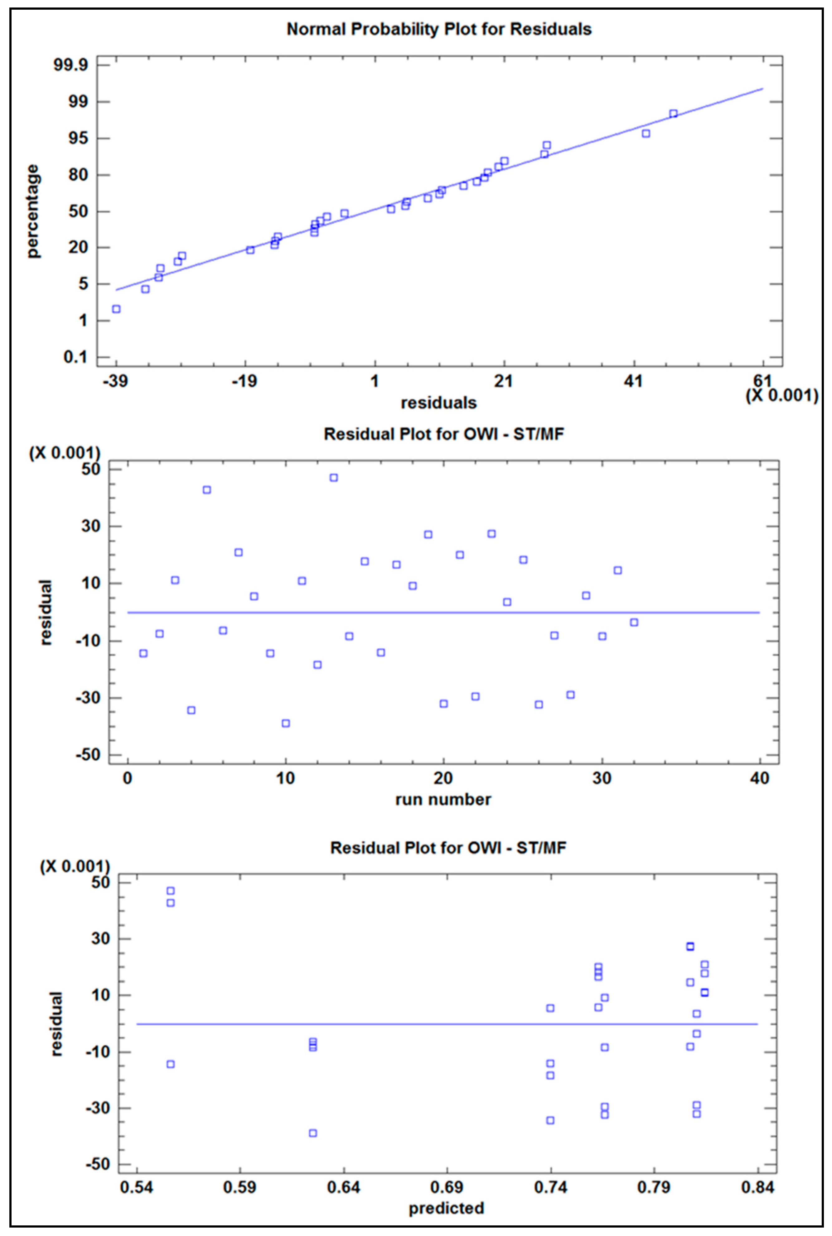
The homoscedasticity plot in Figure 6 did not show any unusual structure. As for Normality verification, a chi-square normality test was performed, where the OWIST, MF residues were distributed into 16 equally probable classes, and each class was then compared with the expected number of observations. Using Statgraphics software for this analysis, a P-value was obtained equal to 0.9273 for this normality test, which is greater than or equal to 0.05. This prevents rejecting the hypothesis that OWIST, MF residues do not come from a normal distribution, with statistical confidence level of 95%.
The assumption of data independence was verified from the plot of Residues vs. Execution order in Figure 6. As in the 2k experiment, the results shown in this figure indicate that the residuals did not follow a trend in terms of their execution order. The plot of residues in Figure 6 suggests that there is no autocorrelation among the residuals of the ANOVA.
After verifying the fit of the qualitative parameters, it can be summarized that the optimal calibration for this case study for the Meta River occurs at these experimental conditions: Van Rijn transport equation; Ks = 0.5 and Kb = 0.1. As result, the modelers obtained an OWIST, MF = 0.8293 and a global OWI = 0.8571.

4.4. Additional Remarks

As previously stated, the method proposed in this paper is based on DOE theory, and because of this, it shares some of its limitations:
  • The domain of quantitative variables must be continuous;
  • It is possible to discard a significant calibration parameter value, because of an inadequate choice of levels or alternatives during the screening design;
  • Some combinations of calibration parameter values might generate numeric instability during the simulation;
  • The lack of replicates (with different results) for the same configuration limits the degrees of freedom of the experiment.
It is also worth noting that the goodness of fit might considerably vary depending on the numeric model used and its capacity to recreate the hydrodynamic, sedimentologic and morphological processes under analysis.

5. Conclusions

By including principles of design of experiments (DOE), the method presented in this paper improves the reliability of the calibration process of hydromorphological models. This becomes even more relevant for rivers whose hydrodynamics depends on morphological processes. Within this context, this paper presented a calibration method based on DOE, which consists of a systematic approach for evaluating the qualitative and quantitative performance of a hydromorphological numerical model based on its corresponding calibration parameters, with the aim of allowing the modelers to get a better understanding and of the effects of these parameters on the adjustment indicators.
Using a 75 km reach of the Meta River as case study, and the MIKE-21C model, the method and its results were described and discussed, along with some of its limitations. The calibration parameters for this case study were the roughness coefficient, the sediment transport equation, the riverbed and suspended load factors, the transverse slope coefficient and the transverse slope power. An optimal overall weighted indicator, which can be defined as an integrated measure of the performance of the model was found for the example, with a value of 85.71%.
The method is versatile in terms of number of calibration parameters and selection of adjustment indicators, because their selection depends on the modeling objective and characteristics of the analyzed section. This method can be applied to unidimensional or multidimensional hydromorphological models.
Based on the findings of this study, some future research directions are:
  • Compare the efficiency of the method and calibration performance by using other DOE types (Fractional Factorials, Taguchi, Latin Square, etc.) and statistical measures of goodness of fit (Nash-Sutcliffe’s efficiency coefficient (NSE), P-Bias, etc.).
  • Compare the performance of the method with other calibration approaches for different conditions: numerical models, river characteristics, quantity and type of calibration parameters, etc.

Author Contributions

Conceptualization, G.J.A. and H.A.; Methodology, G.J.A. and H.A.; Formal Analysis, G.J.A. and H.A.; Writing and Original Draft Preparation, G.J.A. and F.A.C.; Writing, Review and Editing, G.J.A. and F.A.C.; Funding acquisition, H.A.

Funding

This research was funded by the Universidad del Norte, Colombia.

Acknowledgments

The authors acknowledge the teamwork with the Institute of Hydraulic and Environmental Studies of the Universidad del Norte and data from the project “Update of the Studies and Designs for the Navigation of the Meta River between Cabuyaro (K804) and Puerto Carreño (K0)”.

Conflicts of Interest

The authors declare no conflict of interest.

References

  1. Church, M.; Ferguson, R.I. Morphodynamics: Rivers beyond steady state. Water Resour. Res. 2015, 51, 1883–1897. [Google Scholar] [CrossRef]
  2. Yadav, B.; Eliza, K. A hybrid wavelet-support vector machine model for prediction of lake water level fluctuations using hydro-meteorological data. Measurement 2017, 103, 294–301. [Google Scholar] [CrossRef]
  3. Zhu, Q.; Wang, Y.P.; Gao, S.; Zhang, J.; Li, M.; Yang, Y.; Gao, J. Modeling morphological change in anthropogenically controlled estuaries. Anthropocene 2017, 17, 70–83. [Google Scholar] [CrossRef]
  4. Pascolo, S.; Petti, M.; Bosa, S. On the wave bottom shear stress in shallow depths: The role ofwave period and bed roughness. Water 2018, 10, 1348. [Google Scholar] [CrossRef]
  5. Logan, B.L.; McDonald, R.R.; Nelson, J.M.; Kinzel, P.J.; Barton, G.J. Use of Multidimensional Modeling to Evaluate a Channel Restoration Design for the Kootenai River, Idaho; Scientific Investigations Report 2010–5213; U.S. Geological Survey: Reston, VA, USA, 2011.
  6. Stewart, G.; Anderson, R.; Wohl, E. Two-dimensional modelling of habitat suitability as a function of discharge on two Colorado rivers. River Res. Appl. 2005, 21, 1061–1074. [Google Scholar] [CrossRef]
  7. Ouédraogo, W.; Raude, J.; Gathenya, J. Continuous modeling of the Mkurumudzi River catchment in Kenya using the HEC-HMS conceptual model: Calibration, validation, model performance evaluation and sensitivity analysis. Hydrology 2018, 5, 44. [Google Scholar] [CrossRef]
  8. Refsgaard, J.C.; Henriksen, H.J. Modelling guidelines—Terminology and guiding principles. Adv. Water Resour. 2004, 27, 71–82. [Google Scholar] [CrossRef]
  9. Kannan, N.; Santhi, C.; White, M.J.; Mehan, S.; Arnold, J.G.; Gassman, P.W. Some Challenges in hydrologic model calibration for large-scale studies: A case study of SWAT model application to Mississippi–Atchafalaya River basin. Hydrology 2019, 6, 17. [Google Scholar] [CrossRef]
  10. Arsenault, R.; Brissette, F.; Martel, J.L. The hazards of split-sample validation in hydrological model calibration. J. Hydrol. 2018, 566, 346–362. [Google Scholar] [CrossRef]
  11. Hernandez-Suarez, J.S.; Nejadhashemi, A.P.; Kropp, I.M.; Abouali, M.; Zhang, Z.; Deb, K. Evaluation of the impacts of hydrologic model calibration methods on predictability of ecologically-relevant hydrologic indices. J. Hydrol. 2018, 564, 758–772. [Google Scholar] [CrossRef]
  12. Kavetski, D.; Kuczera, G.; Franks, S.W. Calibration of conceptual hydrological models revisited: 1. Overcoming numerical artefacts. J. Hydrol. 2006, 320, 173–186. [Google Scholar] [CrossRef]
  13. Guerrero, M.; Di Federico, V.; Lamberti, A. Calibration of a 2-D morphodynamic model using water–sediment flux maps derived from an ADCP recording. J. Hydroinforma. 2013, 15, 813–828. [Google Scholar] [CrossRef]
  14. Troy, T.J.; Wood, E.F.; Sheffield, J. An efficient calibration method for continental-scale land surface modeling. Water Resour. Res. 2008, 44, 1–13. [Google Scholar] [CrossRef]
  15. Getirana, A.C.V. Integrating spatial altimetry data into the automatic calibration of hydrological models. J. Hydrol. 2010, 387, 244–255. [Google Scholar] [CrossRef]
  16. Francés, F.; Vélez, J.I.; Vélez, J.J. Split-parameter structure for the automatic calibration of distributed hydrological models. J. Hydrol. 2007, 332, 226–240. [Google Scholar] [CrossRef]
  17. Singh, S.; Bárdossy, A. Hydrological model calibration by sequential replacement of weak parameter sets using depth function. Hydrology 2015, 2, 69–92. [Google Scholar] [CrossRef]
  18. Beven, K. Prophecy, reality and uncertainty in distributed hydrological modelling. Adv. Water Resour. 1993, 16, 41–51. [Google Scholar] [CrossRef]
  19. Wright, K.A.; Goodman, D.H.; Som, N.A.; Alvarez, J.; Martin, A.; Hardy, T.B. Improving hydrodynamic modelling: An analytical framework for assessment of two-dimensional hydrodynamic models. River Res. Appl. 2017, 33, 170–181. [Google Scholar] [CrossRef]
  20. Paarlberg, A.J.; Guerrero, M.; Huthoff, F.; Re, M. Optimizing dredge-and-dump activities for river navigability using a hydro-morphodynamic model. Water 2015, 7, 3943–3962. [Google Scholar] [CrossRef]
  21. Wu, K.; Yeh, K.C.; Lai, Y.G. A combined field and numerical modeling study to assess the longitudinal channel slope evolution in a mixed alluvial and soft bedrock stream. Water 2019, 11, 735. [Google Scholar] [CrossRef]
  22. Guan, M.; Liang, Q. A two-dimensional hydro-morphological model for river hydraulics and morphology with vegetation. Environ. Model. Softw. 2017, 88, 10–21. [Google Scholar] [CrossRef] [Green Version]
  23. Kang, T.; Kimura, I.; Shimizu, Y. Responses of bed morphology to vegetation growth and flood discharge at a sharp river bend. Water 2018, 10, 223. [Google Scholar] [CrossRef]
  24. Castro-Bolinaga, C.F.; Fox, G.A. Streambank erosion: Advances in monitoring, modeling and management. Water 2018, 10, 1346. [Google Scholar] [CrossRef]
  25. Bosa, S.; Petti, M.; Pascolo, S. Numerical modelling of cohesive bank migration. Water 2018, 10, 961. [Google Scholar] [CrossRef]
  26. Klein, A. Verification of Morphodynamic Models on Channels, Trenches, and Pits. Master’s Thesis, TU Delft, Delft, The Netherlands, March 2004. [Google Scholar]
  27. Van Waveren, R.H.; Groot, S.; Scholten, H.; van Geer, F.; Wösten, H.; Koeze, R.; Noort, J. Good Modelling Practice Handbook; RWS-RIZA: Lelystad, The Netherlands, 1999. [Google Scholar]
  28. DHI. MIKE 21C Curvilinear model for river morphology—Scientific Documentation. Available online: http://manuals.mikepoweredbydhi.help/2017/Water_Resources/MIKE21C_Scientific_documentation.pdf (accessed on 11 November 2018).
  29. Papanicolaou, A.N.T.; Krallis, G.; Edinger, J. Sediment transport modeling review—Current and future developments. J. Hydraul. Eng. 2008, 134, 1–14. [Google Scholar] [CrossRef]
  30. Mueller, E.R.; Pitlick, J. Sediment supply and channel morphology in mountain river systems: 1. Relative importance of lithology, topography, and climate. J. Geophys. Res. Earth Surf. 2013, 118, 2325–2342. [Google Scholar] [CrossRef]
  31. Sear, D.A.; Newson, M.D.; Thorne, C.R. Guidebook of Applied Fluvial Geomorphology; Thomas Telford Ltd: London, UK, 2010. [Google Scholar]
  32. Matte, P.; Secretan, Y.; Morin, J. Hydrodynamic modeling of the St. Lawrence fluvial estuary. I: Model setup, calibration, and validation. J. Waterw. Port Coast. Ocean Eng. 2017, 143, 04017010. [Google Scholar] [CrossRef]
  33. Chaves, H.M.L.; Alipaz, S. An integrated indicator based on basin hydrology, environment, life, and policy: The watershed sustainability index. Water Resour. Manag. 2007, 21, 883–895. [Google Scholar] [CrossRef]
  34. DHI Water & Environment. MIKE 21 Flow Model FM—User Guide: Sand Transport Module, incl. Shoreline Morphology; DHI Water & Environment: Hørsholm, Denmark, 2017. [Google Scholar]
  35. De Villiers, J. 2D Modelling of Turbulent Transport of Cohesive Sediments in Shallow Reservoirs. Master’s Thesis, University of Stellenbosch, Stellenbosch, South Africa, 2006. [Google Scholar]
  36. Beck, J.S.; Basson, G.R. Klein River estuary (South Africa): 2D numerical modelling of estuary breaching. Water SA 2008, 34, 33–38. [Google Scholar]
  37. Jain, R. The Art of Computer Systems Performance Analysis: Techniques for Experimental Design, Measurement, Simulation, and Modeling, 1st ed.; John Wiley & Sons: Hoboken, NJ, USA, 1991. [Google Scholar]
  38. Montgomery, D.C. Design and Analysis of Experiments, 9th ed.; John Wiley & Sons: Hoboken, NJ, USA, 2017. [Google Scholar]
  39. Kleijnen, J.P.C. Experimental design for sensitivity analysis, optimization, and validation of simulation models. In Handbook of Simulation; Banks, J., Ed.; John Wiley & Sons: Hoboken, NJ, USA, 1998; pp. 173–223. [Google Scholar]
  40. Lee, R. Statistical design of experiments for screening and optimization. Chemie-Ingenieur-Technik 2019, 91, 191–200. [Google Scholar] [CrossRef]
  41. Dorfmann, C.; Knoblauch, H. ADCP measurements in a reservoir of a run-of-river Hydro Power Plant. In Proceedings of the 6th International Symposium on Ultrasonic Doppler Methods for Fluid Mechanics and Fluid Engineering, Prague, Czech Republic, 9–11 September 2008; pp. 45–48. [Google Scholar]
  42. Universidad del Norte. Actualización de los Estudios y Diseños para la Navegabilidad del río Meta entre Cabuyaro (K804) y Puerto Carreño (K0); Universidad del Norte: Barranquilla, Colombia, 2013. [Google Scholar]
  43. Plan Maestro Fluvial de Colombia 2015; Ministerio de Transporte: Bogotá, Colombia, 2015.
  44. Caracterización del Transporte en Colombia—Diagnóstico y Proyectos de Transporte e Infraestructura; Ministerio de Transporte: Bogotá, Colombia, 2005.
  45. Pasternack, G.B.; Gilbert, A.T.; Wheaton, J.M.; Buckland, E.M. Error propagation for velocity and shear stress prediction using 2D models for environmental management. J. Hydrol. 2006, 328, 227–241. [Google Scholar] [CrossRef]
  46. Talmon, A.M. Bed Topography of River Bends with Suspended Sediment Transport. Ph.D. Thesis, Delft University of Technology, Delft, The Netherlands, 1992. [Google Scholar]
  47. DHI Water & Environment. MIKE 21 Flow Model—User Guide: Hydrodynamic Module; DHI Water & Environment: Hørsholm, Denmark, 2017. [Google Scholar]
  48. García, M.H. Sediment transport and morphodynamics. In Sedimentation Engineering; American Society of Civil Engineers: Reston, VA, USA, 2008; pp. 21–163. [Google Scholar]
  49. Engelund, F.; Hansen, E. A monograph on sediment transport in alluvial streams; Technical University of Denmark: Copenhagen, Denmark, 1967. [Google Scholar]
  50. Yang, C.T. Incipient motion and sediment transport. J. Hydraul. Div. 1973, 99, 1679–1704. [Google Scholar]
  51. Van Rijn, L.C. Sediment transport, part II: Suspended load transport. J. Hydraul. Eng. 1984, 110, 1613–1641. [Google Scholar] [CrossRef]
  52. Hidroconsultas LTDA. Estudios básicos en el río Meta para la línea base de ingeniería tendiente a definir el sistema más adecuado para el mantenimiento de un canal navegable, obras de encauzamiento y demás obras fluviales entre la desembocadura del río Casanare y Puerto Texas; Hidroconsultas LTDA: Bogota, Colombia, 2003. [Google Scholar]
Figure 1. Flowchart describing the calibration process.
Water 11 01382 g001
Figure 2. Representative section of the river, between K235–K310.
Water 11 01382 g002
Figure 3. Velocity vectors from the model for hydrodynamic calibration.
Water 11 01382 g003
Figure 4. Normal Probability of Effects for the weighted indicator of sedimentological and morphological adjustment (OWIST, MF) in experimental design 2k.
Water 11 01382 g004
Figure 5. Graphic verification of Homoscedasticity, Normality, and Independence—Experiment 2k.
Water 11 01382 g005
Figure 6. Graphic verification of Homoscedasticity and Independence—Experiment 3k.
Water 11 01382 g006
Figure 7. Comparison between Velocity Vectors in two sections of the reach for the optimal case.
Water 11 01382 g007
Table 1. Typical calibration parameters. (Source: Adapted from [28]).
ComponentParameterDescription
Hydrodynamics
  • Bed resistance to flow
This is related to the riverbed’s resistance to flow. For MIKE-21C, the value at each cell is determined as a function of water depth and Manning’s or Chézy’s coefficient. The model uses as input a constant value or maps corresponding to their spatial distribution.
  • Eddy viscosity—K
Parameter related to the calibration of the velocity vector and depends on the turbulence state. For MIKE-21C, usually between 0.2 m2/s and 5.0 m2/s.
Sedimentology/ Morphology
  • Sediment transport equation
The selection of sediment transport equation defines the parameters to be used in the model, and it mainly depends on granulometry (i.e., particle size and shape). A complete description of the transport formulae can be found in the MIKE-21C user’s guide [28].
  • Bed load factor—Kb
  • Suspended load factor—Ks
The total sediment load is estimated through a sediment transport equation (MIKE-21C includes a set of options for this purpose).
  • Longitudinal slope coefficient—LSC
  • Transverse slope coefficient—TSC
  • Transverse slope power—TSP
These parameters modify sediment transport rates in the stream current, considering morphological changes affecting transverse and longitudinal slopes.
  • Helical flow calibration constant—HL
In MIKE-21C this parameter defines the intensity of the helical flow on the riverbed due to the secondary currents. It is usually assumed to be equal to 1; however and ranges from 0.4 to 1.2, according to [34].
  • Erosion rate on riverbanks
According to MIKE-21C, the erosion rate on the riverbanks can be calibrated using three different parameters,
α : Transversal slope of the riverbank.
ψ : Fraction of sediment transport rate near the bank.
γ : Erosion constant which does not depend on the hydraulic condition.
Table 2. Flow distribution through river branches around islands of the river reach.
Abscissa (km)ArmObservedC = 50C = 55C = 60
204Right0.70760.68750.69150.6962
Left0.29240.31250.30850.3038
289Right0.15980.17570.16940.1514
Left0.84020.82430.83060.8486
267Right0.25800.27180.24530.2516
Left0.74200.72820.75470.7484
248Right0.05600.05270.04360.0327
Left0.94400.94730.95640.9673
Table 3. Hydrodynamic calibration results.
CR2OWIHD
Water Level (WL)Flow Distribution (FD)
500.78930.99790.8727
550.84500.99810.9062
600.82720.99840.8957
Table 4. Factors (Calibration parameters) for 2k experimental design.
LevelSediment Transport Equation (A) *Suspended Load Factor—Ks (B) *Riverbed Load Factor Kb (C) *Transverse Slope Coeff.—TSC (D) *Transverse Slope Power—TSP (E) *
HighYang0.10.10.6250.5
LowVan Rijn0.90.51.2501.0
* The letters in parentheses will be used to abbreviate the name of the corresponding calibration parameters.
Table 5. Analysis of Variance (ANOVA) results for the 2k experiment.
SourceSum of SquaresDfMean SquareF-RatioP-Value
A: Transport Eq0.08440010.084400245.660.0000
B: Ks0.10630010.106300309.350.0000
C: Kb0.00740010.00740021.760.0001
AB0.04020010.040200117.230.0000
BC0.01020010.01020029.900.0000
ABC0.01020010.01020029.670.0000
Total error0.008200240.000340
Total (corrected)0.26720031
Table 6. Factors (Calibration parameters) for 3k experimental design.
LevelSediment Transport Equation (A)*Suspended Load Factor—Ks (B)*Riverbed Load Factor Kb (C)*
HighYang0.10.1
Mid-0.50.3
LowVan Rijn0.90.5
Table 7. ANOVA results for the 3k experiment.
SourceSum of SquaresDfMean SquareF-RatioP-Value
A: Transport Eq0.103394010.103394091.530.0000
B: Ks0.066686620.033343329.520.0000
C: Kb0.019697720.00984898.720.0016
AB0.028154220.014077112.460.0002
BC0.013497720.00674895.970.0085
ABC0.023132440.00578315.120.0045
Total error0.0248521220.0011296
Total (corrected)0.279415035