Article

Spatially Explicit Modeling of Coupled Water and Carbon Processes Using a Distributed Ecohydrological Model in the Upper Heihe Watershed, China

1
School of Remote Sensing and Geomatics Engineering, Nanjing University of Information Science and Technology, Nanjing 210044, China
2
State Key Laboratory of Resources and Environment Information System, Institute of Geographic Sciences and Natural Resources Research, Chinese Academy of Sciences, 11A, Datun Road, Chaoyang District, Beijing 100101, China
3
College of Resources and Environmental, University of Chinese Academy of Sciences, No. 19A, Yuquan Road, Beijing 100049, China
4
Jiangsu Center for Collaborative innovation of Geographical Information Resources Development and Application, Nanjing 210023, China
5
Institute of Surface-Earth System Science, Tianjin University, Tianjin 300072, China
*
Author to whom correspondence should be addressed.
Water 2019, 11(6), 1242; https://doi.org/10.3390/w11061242
Submission received: 22 May 2019 / Revised: 10 June 2019 / Accepted: 12 June 2019 / Published: 13 June 2019
(This article belongs to the Section Water Quality and Contamination)

Abstract

:
A fully coupled simulation of ecophysiological, hydrological and biochemical processes is significant for better understanding the individual and interactional impact of sophisticated land surface processes under future disturbances from nature and human beings. In this study, we spatially explicitly modelled evapotranspiration (ET) and photosynthesis (GPP) using a distributed hydrological model, Dynamic Land Model DLM-Ecohydro, over the Upper Heihe watershed for the years of 2013 and 2014. After considering the lateral water movements, the model fairly captured the variations in ET (R2 = 0.82, RMSE = 1.66 mm/day for 2013; R2 = 0.83, RMSE = 1.53 mm/day for 2014) and GPP (R2 = 0.71, RMSE = 5.25 gC/m2/day for 2013; R2 = 0.81, RMSE = 3.38 gC/m2/day for 2014) compared with the measurements from the Arou monitoring station. Vegetation transpiration accounted for total ET of around 65% and 64% in 2013 and 2014, respectively. A large spatial variability was found in these two indicators (14.30–885.36 mm/year for annual ET and 0–2174 gC/m2/day for annual GPP) over the watershed. Soil texture and vegetation functional types were the major factors affecting ET and GPP spatial variability, respectively. The study manifested a coupled water–carbon mechanism through the strong linear relationship between the variations in ET and GPP and the control of hydrological processes on the carbon cycle at the watershed scale. Although the model had a reasonable performance during most parts of the growing seasons, the lack of a soil freezing–thawing scenario caused inevitable discrepancies for the simulation of soil water and heat transfer mechanisms, hence inaccurately estimating the biophysiological processes in the transition period of winter to spring, which should be further improved especially for alpine regions.

1. Introduction

The land surface ecological processes significantly affect the cycling of energy, mass and moisture between the soil, vegetation and atmosphere. These dynamics also make the land surface an important energy and moisture source, sink and reservoir, and hence contributed a lot to terrestrial and climate systems [1,2]. However, the sophistication of individual, and interactions between, hydrological, ecophysiological and energy cycles are hard to comprehend because of the related nonlinear feedback mechanisms, especially for landscape-scaled ecohydrological processes and the uncertainty of natural and anthropogenic disturbances [3]. The tight linkage between water and carbon dynamics is expressed in many hydrologically controlled ecological processes, for instance, respiration [4], photosynthesis [5], water use efficiency [6] and crop coefficient analyses [7].
Currently, there are many ecophysiological modeling researches published at multiple spatio-temporal resolutions and spans, including point scales [8,9], mesoscales [10,11] and global scales [12] at yearly [13] or minute time-steps [1], while few of them completely considered the soil water processes and the non-linear relationship between it and vegetation ecophysiological processes. Due to the limited understanding of water–carbon interactions, many researches (regardless of modeling or measurement) often regard them as an isolated process [2]. At mesocales, especially for the watershed scale, where the land surface ecological processes are highly sensitive to local water balance, topography is an important contributor for local water cycling and, furthermore, ecophysiological processes. Many researches [14,15,16] suggested that the overlook of topographical-controlled lateral water fluxes would cause significant biases in local estimation of water (evapotranspiration, runoff and soil moisture) and carbon fluxes (GPP: Gross primary productivity, NPP: Net primary productivity and NEP: Net ecosystem productivity). For the traditional hydrological models, although they can completely consider the watershed hydrological processes, they always neglect or simplify the impact of vegetation on soil water and their ecophysiological processes.
Evapotranspiration (ET) and photosynthesis (as GPP) are two critical ecophysiological processes for the connection between land surface water, energy and carbon cycling, and both of them are highly governed by local soil hydrological processes. For GPP, the surrounding water content of the rhizome controls photosynthesis efficiency through the effect of vegetation stomatal and enzyme activity [17]. ET has a stronger interaction with the local water and energy balance. About 70% of the precipitation that falls on the land surface gets back to the atmosphere by vegetation ET, and in arid areas ET loss can be up to 90% [18]. Simultaneously, because vaporization and sublimation would take the absorption of heat, it is also important for local thermal balance. The coupling of water and carbon cycling can better explain these ecohydrological processes and, therefore, help make more efficient decisions for local environmental management.
The Heihe River is the second largest inland river in northwest China and originates from the Qilian Mountains which is in the northern margin of the Tibetan Plateau. It is located in the center of the Eurasian continent, playing an important role in the ancient Silk Road [19]. The upper stream of the watershed takes up around 7% of the Heihe basin area, and is the water source of the whole basin with a wide distribution of grassland which plays a significant role for local carbon assimilation and water cycling [20]. Influenced by the westerly belt circulation and the cold continental polar air mass, the Upper Heihe watershed has an arid to semiarid climate with scarce and concentrated precipitation [21,22]. The water shortage and complex topography are major reasons for sparse vegetation coverage, and hence a more fragile ecological environment [23]. Hitherto, the estimations of ET and GPP in the Upper Heihe watershed were isolated. Yang [24] utilized micro-lysimeters to test the performance of four energy balance methods for ET estimation in the meteorological station of Qilian Mountains, and found that the FAO-56 Penmen-Monteith provided the highest accuracy. Wang [25] established the relationship model between four stations’ eddy-covariance-based GPP and the leaf area index (LAI), with vegetation indexes extracted from Moderate Resolution Imaging Spectroradiometer (MODIS) in the Heihe River basin. Yan [20] utilized a remote sensing-based light use efficiency model (MODIS MOD_17) to simulate the GPP of the Upper Heihe watershed, and found that temperature and vapor pressure deficiency had a positive relationships with GPP. These researches lack the description of an ecological water and carbon-coupled mechanism, neither considering the effect of rhizosphere soil water on carbon assimilation rate, nor considering the feedback of the soil carbon pool, biological carbon pool and vegetation growth on the ecosystem water cycle. Sun [26] compared the performance of two land surface models—Community Land Model 4.0 (CLM 4.0) and Dynamic Land Model 1.0 (DLM 1.0)—in the simulation of soil organic carbon of the Upper Heihe watershed, and found that these land surface modes had low accuracies for soil moisture estimation in this cold alpine region. The coupling of the distributed-hydrological and traditional biological models is needed for the watershed scale ecophysiological simulation, because it considers not only the microclimate and topographically controlled soil water movement, but also vegetation-unique ecophysiological characters.
This study utilized a process-based ecohydrological model (DLM-Ecohydro) to simulate two ecophysiological processes, evapotranspiration and photosynthesis, in the cold alpine region. We will test how the model performed after considering topographically controlled lateral water movement and the coupling of the water cycle and carbon assimilation at daily time steps. Through the study of spatiotemporal differentiation of ET and GPP in the Upper Heihe watershed, we will also explore the driving mechanism of ecosystem water and carbon flux variations.

2. Materials and Methods

2.1. Study Area

The eco-hydrological simulation focused on the Upper Heihe watershed which covers around 10,009 km2 in the northeastern part of the Tibetan Plateau, China (Figure 1). The distributions of precipitation and landscapes have strong spatial heterogeneity with a significant topographic relief (from 1600 to 5100 m above sea level). The annual precipitation ranges from 250 mm in lower altitude areas, to 500 mm in higher zones. Melting water from glaciers and snow effectively compensates surface overland and subsurface runoff during spring and early summer [27]. The Upper Heihe watershed is a classical alpine-cold climate with most of the typical landscapes of cold regions, include alpine grassland, alpine meadow, forest, glacier, barren and so on. According to Qin [28], more than 98% of forests fall in the 2000–4000 m a.s.l. area in the watershed. Glaciers lie in places over 4500 m a.s.l. and takes up around 3.4% of the whole watershed area. Grassland and shrubland are mainly distributed in the 1700–4900 m a.s.l. and 2900–5066 m a.s.l. areas, respectively. The annual temperature of the Upper Heihe watershed is lower than 2 °C. Biogeographically, solar and topographic condition are important factors which control the composition of vegetation species. In terms of grassland, Reaumuria soongorica and Sympegma regelu are the main species on sunny slopes, while for shady slopes, it majorly consists of Polygonum viviparum and Carex atrata [29]. Clay is the major soil type within the watershed.

2.2. Model Discription

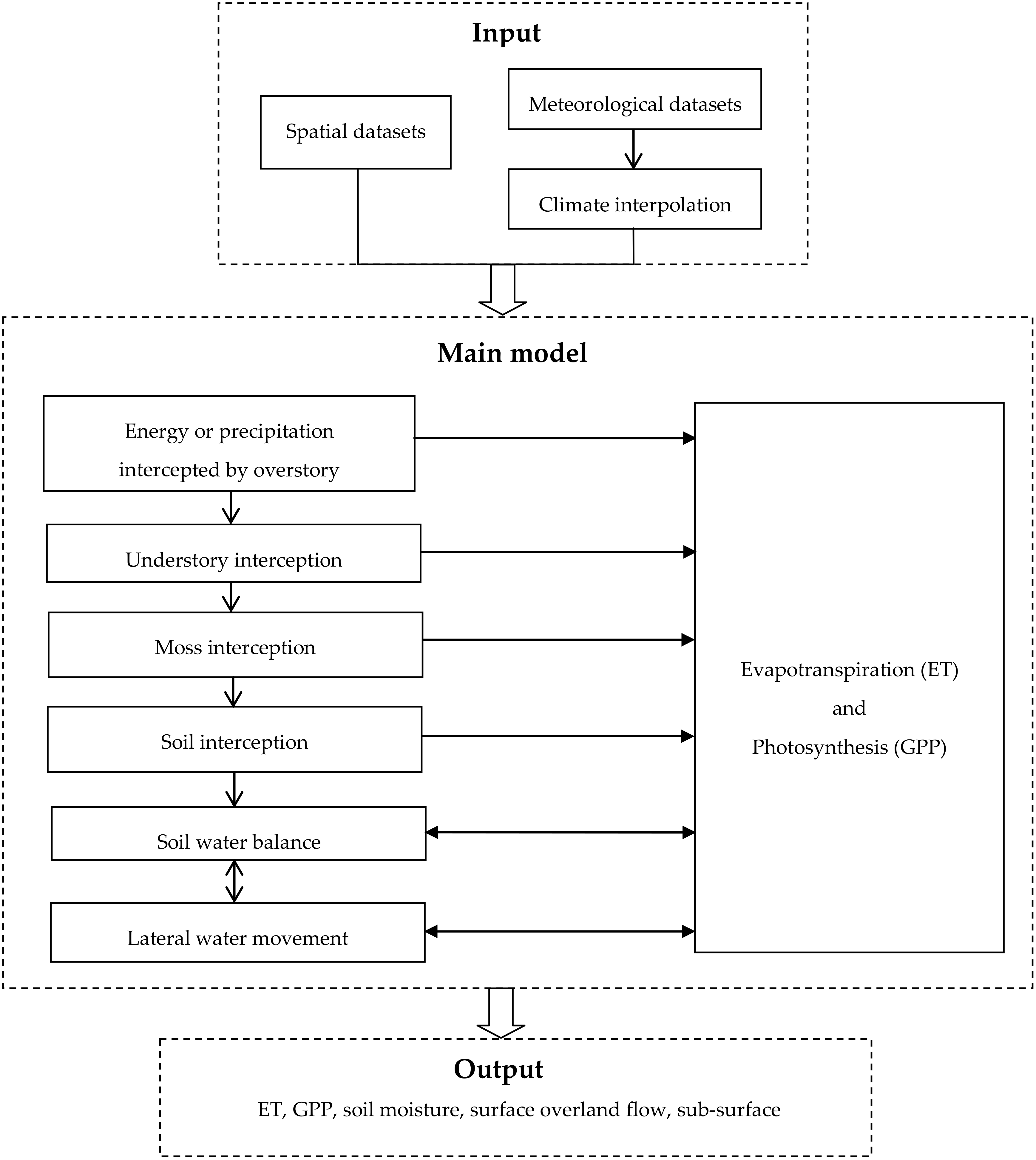
This study utilized a processed-based model, DLM-Ecohydro, which was developed from the Boreal Ecosystem Productivity Simulator (BEPS)-TerrainLab V2.0 [15] and DLM [30]. It modified the modeling period of BEPS-TerrainLab V2.0 from one year to multi-year and localized the vegetation characters for an arid-cold mountain region. Depending on the input datasets, the model is able to resample and run at any spatial resolution. It is carried out using a “four-leave” approach to separate leaf stratifications according to different soil moisture and sunshine states and then spatially upscaled from the leaf to the canopy level. Figure 2 shows a flow chart of the model. Under the input datasets, the model obtains the necessary meteorological and geological conditions, the biophysiological characteristics of local vegetation and the initial ecohydrological status of the watershed. The input energy and precipitation to ecosystem are intercepted according to a hierarchical order at the canopy scale. Rather than a simple bucket model used in Boreal Ecosystem Productivity Simulator (BEPS), DLM-Ecohydro completely considers the effects of lateral fluxes on the above ecophysiological processes by solving a water balance equation. After considering the interactions between ecosystem energy, biochemical and hydrological processes, the model could fairly represent the dynamic states of ecological and hydrological indicators.

2.2.1. Ecophysiological Processes

The DLM-Ecohydro model separates canopy into overstory, understory, moss and soil surface. According to different light conditions and soil moistures states of the rhizosphere, the leaves of each part were divided into sunlit and shade, saturated and unsaturated states. Taking overstory canopy, for example, the conceptualizations of leaf-specific physiological processes is listed as follows:
P o , sun , sat = f x R sun , g s , sun , sat , P o , sun , unsat = f x R sun , g s , sun , unsat , P o , shade , sat = f x R sahde , g s , shade , sat ,   and P o , shade , unsat = f x R shade , g s , sahde , unsat ,
where Po is overstory canopy transpiration or photosynthesis from: Sunlit leaves with saturated soil water condition (Po,sun,sat); sunlit leaves with unsaturated soil water conditions (Po,sun,unsat); shaded leaves with saturated soil water condition (Po,shade,sat); and shaded leaves with unsaturated water condition (Po,shade,unsat). Function fx can be either the Penman-Monteith equation for each sub-component of ET (except for sublimation) or the Farquhar model [31] for GPP simulation. R is overstory net radiation for ET and short wave radiation for GPP calculation for sunlit (Rsun) or shaded (Rshade) leaves; gs, overstory stomatal conductance of H2O and CO2 for ET and GPP, respectively, from: Sunlit leaves with saturated soil water condition (gs,sun,sat); sunlit leaves with unsaturated soil water conditions (gs,sun,unsat); shaded leaves with saturated soil water condition (gs,shade,sat); and shaded leaves with unsaturated water condition (gs,shade,unsat). The up-scaling scheme employed a specific LAI and root fraction as weighting terms, expressed as follows:
P o = P o , sun , sat × LAI sunlit × µ o + P o , sun , unsat × LAI sunlit × 1 µ o + [ P o , shade , sat × LAI shade × µ o + P o , shade , unsat × LAI sahde × 1 µ o ] ,
where Po is overstory canopy ET or GPP, and LAI is the function of the solar zenith angle to divide sunlit (LAIsunlit) and shaded (LAIshade) leaves. µo represented overstory roots in the unsaturated zone and (1 − µo) was that in the saturated zone. The fraction of root µ was the function of the root extinction coefficient and water table depth based on the specific pixel and Julian day [32]. The upscaling scheme defaulted the understory canopy just as has shaded leaves. There was no upscaling of soil surface physiological processes because the model deemed it as a single layer with ground specific radiation and soil conductance.

2.2.2. Water Balance Calculation

In the DLM-ecohydro model, the detailed water balance equation considers the lateral water flux by the description of surface overland floor (Fsurface) and sub-surface baseflow (Fsubsurface) at the pixel scale and daily time steps. Once the infiltration process reaches its max capacity [33], the ponded water would appear on the soil surface and move laterally as Fsurface. The topography derived lateral subsurface baseflow is the difference between subsurface inflow and outflow within eight neighboring pixels as described in [15]. Water balance calculations are composed with storage changes at unsaturated (ΔWunsat) and saturated (ΔWsat) soil parts which are presented below:
Δ W unsat = I F surface + C P T unsat E floor ,
Δ W sat = P F subsurface T sat C ,   and
Δ W = I F surface F subsurface T unsat T sat E floor
where I is total infiltrated water which is comprised of through-fall, snowmelt and stem flow [34], P is percolation and represented the water in the unsaturated zone downward to the saturated part under the impact of gravity, while C is capillary rise upward from the saturated to vadose zone appearing under extreme surface dryness. Tunsat and Tsat are the transpirations from roots situated in the unsaturated and saturated zones, respectively. Efloor is soil evaporation and sublimation of snowpack. The complete soil profile storage change is the sum of two soil zones (Equation (5)).

2.3. Data Preparation

2.3.1. Spatial Datasets and Model Initialization

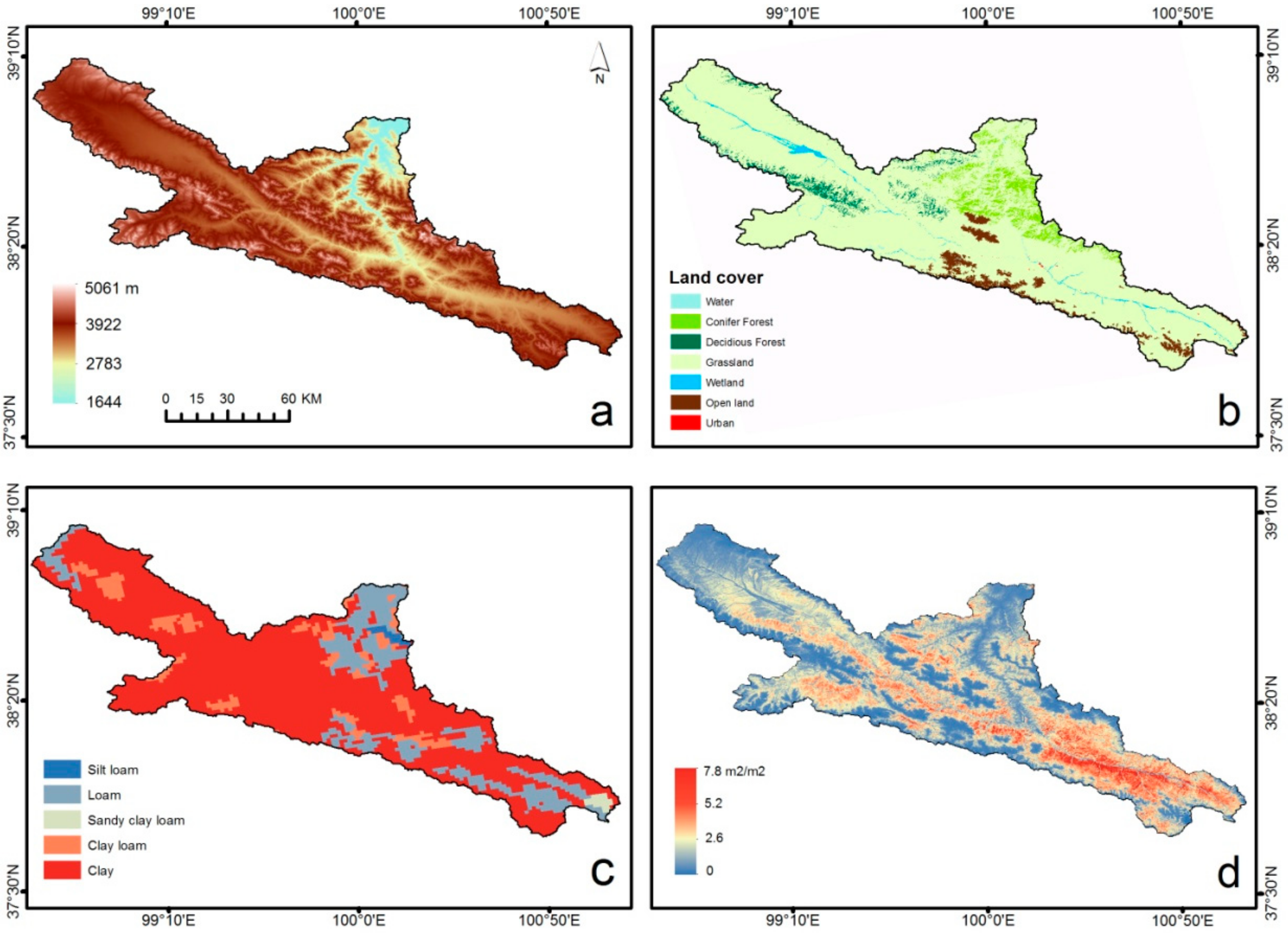
Most of the spatial datasets were generated based on the combination of GIS, remote sensing, field monitoring and modeling. All of these datasets were resampled to the same spatial resolution (100 m × 100 m) and projected in World Geodetic System-1984 Coordinate System (WGS-84). The digital elevation model (Figure 3a) was obtained from a 30 m Advanced Spaceborne Thermal Emission and Reflection Radiometer Global Digital Elevation Model (ASTER GDEM) dataset. It was crucial for the computing of lateral hydrological processes and spatial interpolation of various meteorological parameters. Watershed land cover (Figure 3b) was obtained from a 30 m global LC dataset, GlobaLand30, and merged as part of the classifications to fit DLM-Ecohydro. After model parameters localization and optimization, the biophysical parameters for the major land cover types in the Upper Heihe watershed are shown in Table 1. A soil texture map (Figure 3c) was obtained from a 1 km Harmonized World Soil Database (HWSD) dataset established by the FAO and IIASA. The key hydraulic properties of the four main soil types in the Upper Heihe watershed are shown in Table 2. The watershed annual maximum LAI (Figure 3d) was generated from Moderate Resolution Imaging Spectroradiometer (MODIS) LAI production (MOD15A2), July 2013. In addition to the spatial datasets above, an initial water table depth (WTD) and ecosystem C-pools (including four biomass C-pools and nine soil C-pools) were necessary for the eco-hydrological and biogeochemical module of DLM-Ecohydro. We used CLM4.0 [35] to spin up WTD based on 2013 meteorological and topographical data, and similar iteratively running processes for current sizes of ecosystem carbon pools were based on the CLM4.0 biogeochemical module. The spun up WTD and ecosystem carbon pools were input as 2013 initial datasets and subsequently used for two years of simulation.

2.3.2. Meteorological Datasets and Flux Measurement

The input meteorological datasets included daily maximum, minimum and average temperature (°C), median dew point (°C), total precipitation (mm), wind speed (m/s) and total short-wave radiation (W/m2). These datasets were derived from the Heihe Warershed Allied Telemetry Experimental Research (HiWATER) at the Arou Superstation, which is located in the southeastern part of the study area (100.46° E, 38.05° N) [36,37]. Except for the input datasets above, the energy and carbon fluxes and soil moisture data were also prepared for model validation. Simulated volumetric soil water content (VSWC) were compared with a 0–40 cm average measurement with cosmic-ray probes buried at the Arou station, with a footprint scale of 700 m in diameter [38]. The eddy covariance (EC) technique was used in the Arou footprint tower for continuous and long term monitoring of energy and CO2 fluxes. GPP was derived from the fluxes of net ecosystem exchange (NEE) measured at the EC tower. Based on the Lloyd–Taylar model [39], the relationship between temperature and respiration during the night was used to estimate the daylight respiration rate, thereafter GPP flux could be detected from monitored NEE. The evapotranspiration was converted from measured latent heat fluxes (LE, W/m2) as shown below, where λ is 2.501 × 10⁶ J/kg from [35].
ET = LE / λ .

3. Results and Discussion

3.1. Temporal Patterns of Hydrological Indicators

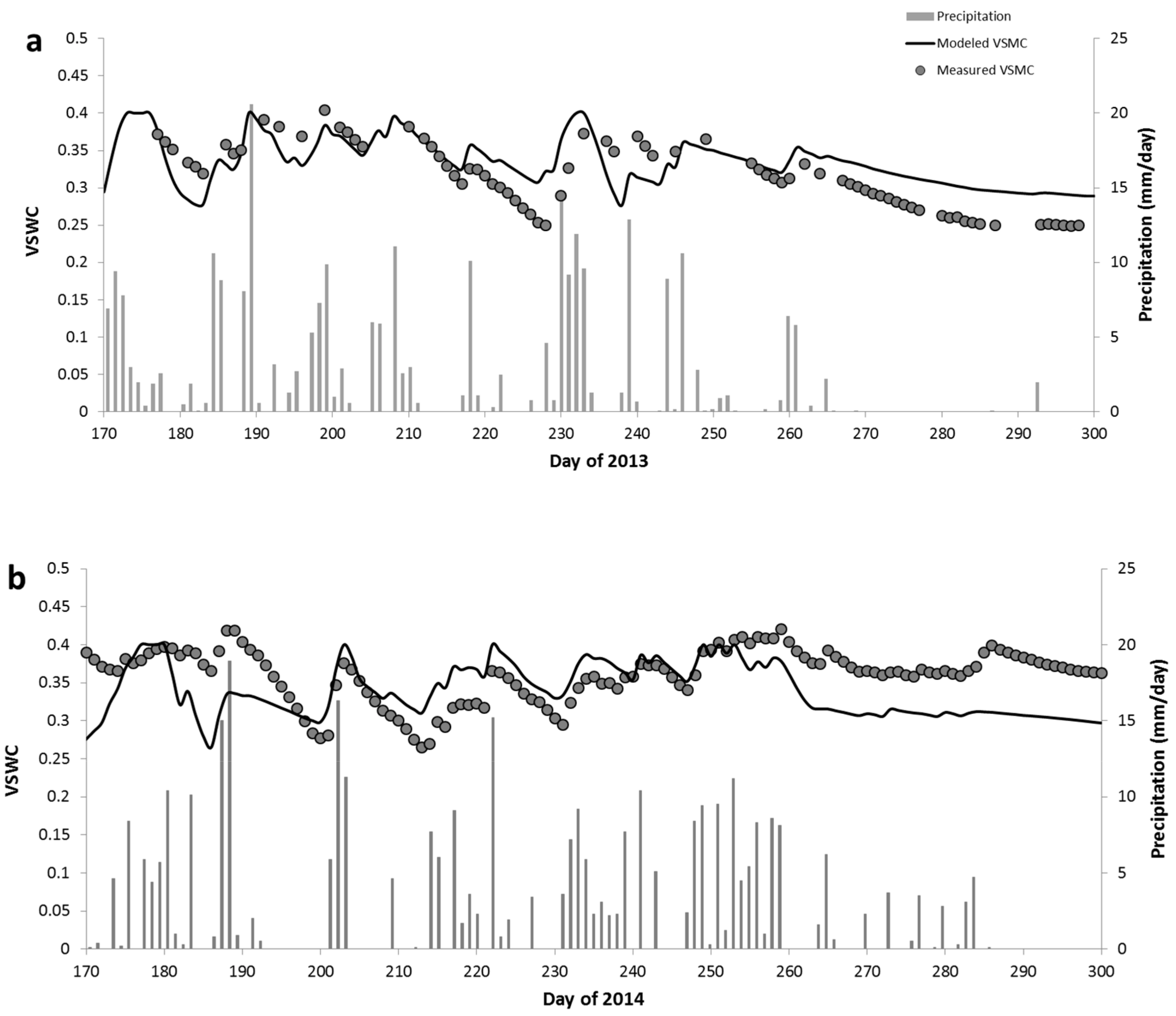
Volumetric soil water content (VSWC) was affected by precipitation, melting runoff, soil temperature and other hydrological or meteorological factors. The model was able to capture the reasonable magnitude and fluctuation of VSWC during most parts of the growing seasons. Figure 4 reveals that the VSWC was between 0.25–0.45 from day of the year (DOY) 170 to DOY 300 and rapidly responded to daily precipitation at the Arou station. The VSWC reached to field capacity (0.4) around DOY 190 of both years because of the adequate water input from snow melting and rainfall. While experiencing days lacking precipitation (DOY 210–230 of 2013; DOY 190–215 of 2014), the VSWC dropped under the permanent wilting point (0.27). And during this time, ecosystem evapotranspiration and lateral water fluxes were the major reasons for soil water losses. There was a dense precipitation after DOY 230 which made the VSWC remain over field capacity. On the other hand, 2013 experienced a prolonged drier autumn that induced a gentle but continuous fall down of VSWC until below the permanent wilting point. While the model overestimated the VSWC during spring and winter when the soil was in a frozen state, it was probably because the model did not take the soil freezing–thawing process into consideration. During the soil frozen period, the permeability would decrease and soil hydraulic characteristics would consequently change. Rather than infiltrated into soil profile, most of the precipitation would drain out as surface overland flow. The lack of these dynamic transformations in the model domain might trigger an unrealistic estimation for soil moisture state. The study area is located in the cold alpine region where the negligence of melting runoff from glaciers and accumulated snowpack might cause the underestimation of soil water especially during spring and early summer.
Figure 5 shows the temporal patterns of two years of lateral water fluxes in the Arou site. On account of the lack of validation data, we only compared it with the daily precipitation. The model captured a rapid response of lateral water fluxes to precipitation in spring and early summer. Under a denser precipitation, the lateral water fluxes of 2014 were much higher than that of 2013. Because in DLM-Ecohydro the surface overland flow (SOLF) was estimated only when saturated water diffuses up to the land surface, i.e., WTD ≤ 0, subsurface baseflow ( SSB) took the major part of the lateral hydrological fluxes. It could reach to 9 mm/day in 2013 and 10 mm/day in 2014 during May and June, respectively. This simulation is more suitable for the soil texture with high hydraulic conductivity, while for clay, it might underestimate the SOLF during dense rainfall periods when the infiltration rate is much lower than the precipitation rate.

3.2. Spatial and Temporal Patterns of ET

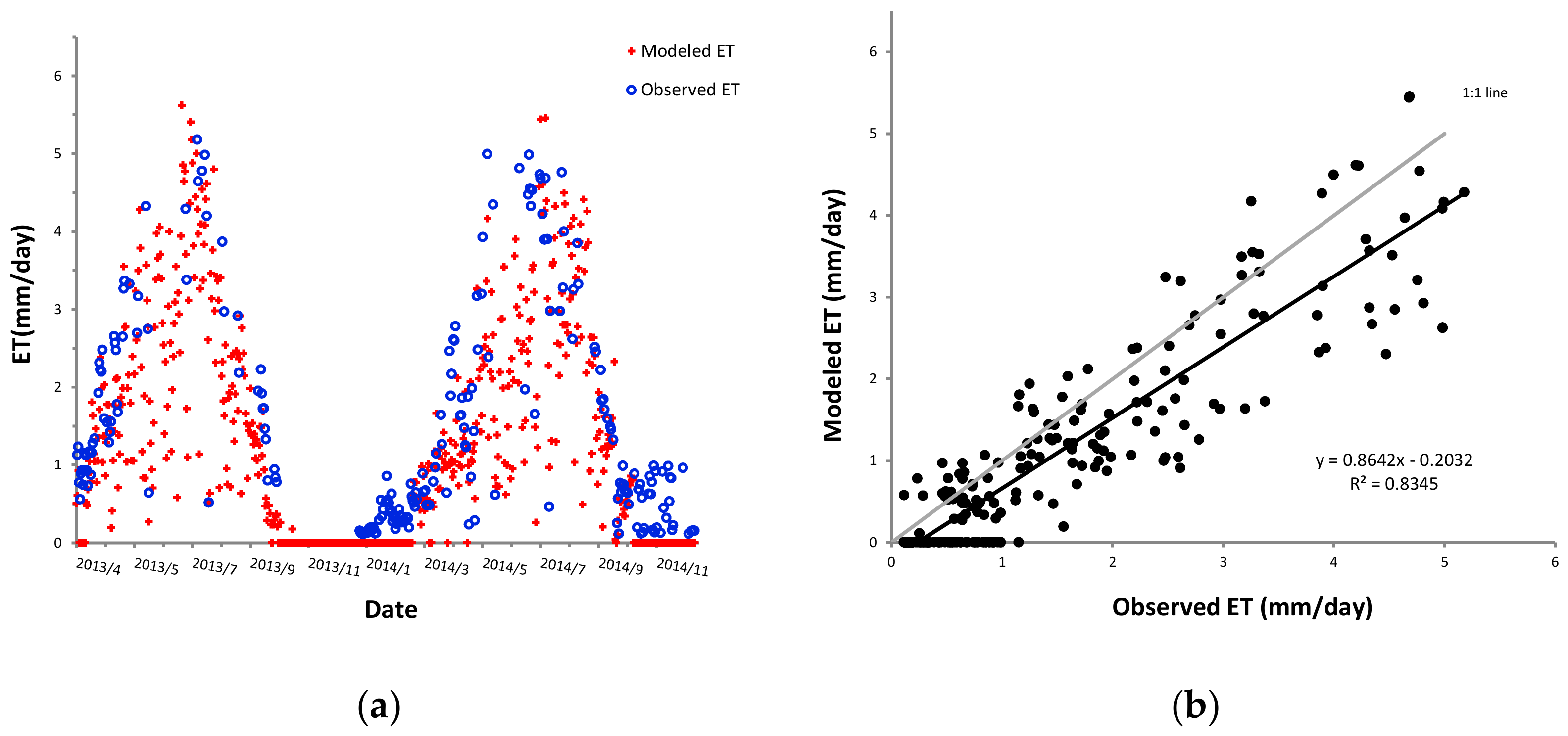
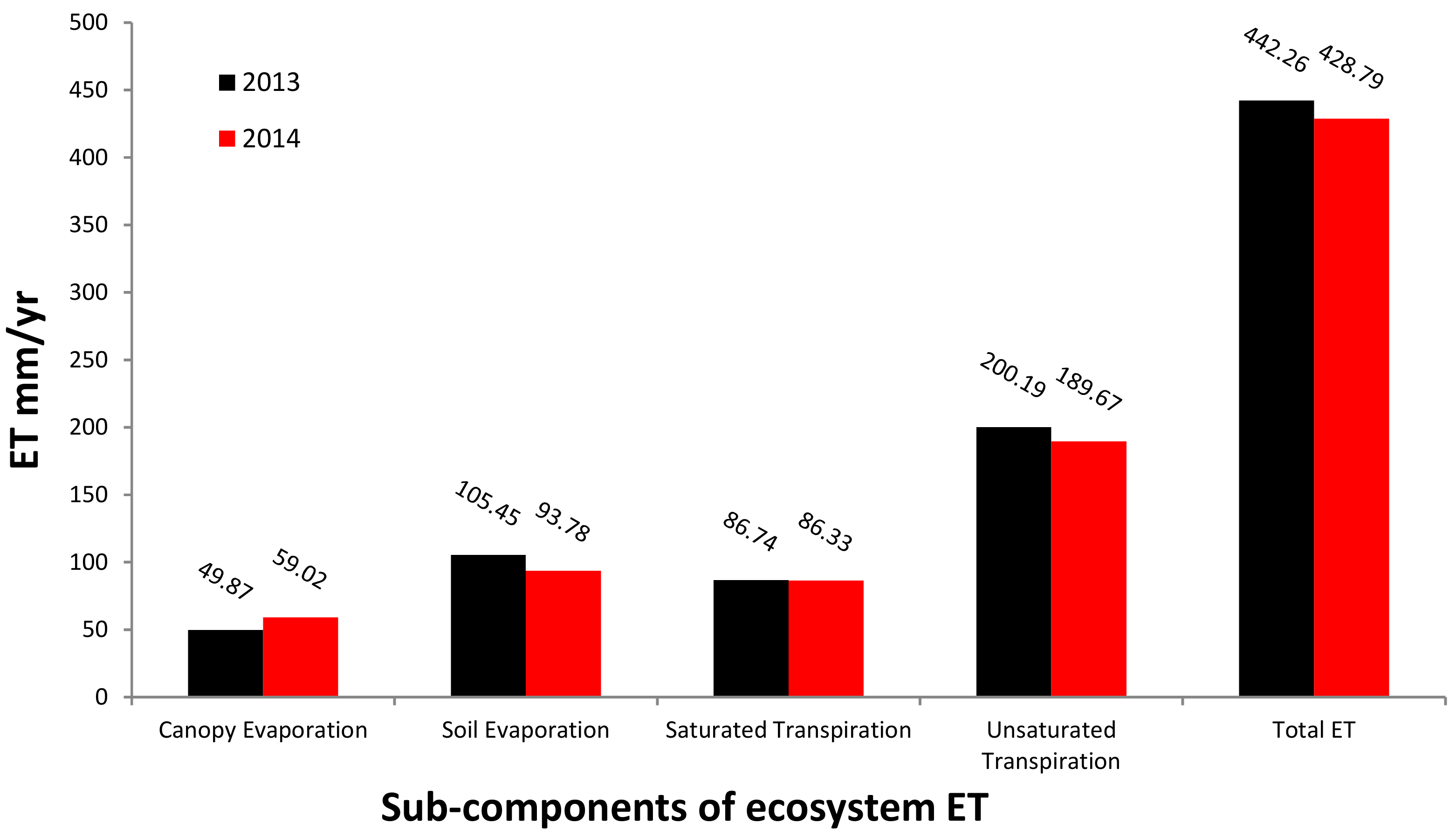
The temporal patterns and magnitudes of ET are well simulated through the DLM-Ecohydro model, which were able to explain 82% (RMSE = 1.66 mm/day) and 83% (RMSE = 1.53 mm/day) of the variability in 2013 and 2014, respectively. The model agilely captured the seasonal patterns of ET losses at the Arou station of both years: With a fluctuated rise during the early summer until up to the top magnitude (around 5 mm/day) at mid-summer and then decrease to lower than 1 mm/day within September and October (as shown in Figure 6). Although the model could capture most of the variation during a year, there was a general underestimation especially in the winter and early summer. One possible reason for winter ET underestimation was the snow sublimation might cause an increase of latent heat measured through the EC tower. Snowfall is a crucial part of the ecosystem water cycle in the Tibetan Plateau of China [40], which has quite a number of accumulated snowpack during winter. According to the findings of Molotch [41], there could be a rapid response of the EC tower to detect the intercepted snow sublimation from the upper canopy. This contributed to a higher observed ET that the model underestimated. At the same time, the only water input of the DLM-Ecohydro model was precipitation which converts to rainfall or snowpack accumulation depending on air temperature. However, above 4500 m a.s.l. alpine region, ice and snowpack covered all year, which induced an increased snowmelt runoff during spring and summer. Li and Wang [42], utilizing snowmelt runoff model (SRM), demonstrated that May and June are major melting months, and the melting runoff can take more than 50% of the total runoff in the Upper Heihe watershed. The negligence of melting runoff from high altitude snow/ice pack might contribute to the considerable underestimation during early summer. One the other hand, the model calculated plant stomatal conductance with the ambient air temperature, while considering the freezing–thawing process in alpine cold regions, the change of soil temperature usually lagging behind that of air temperature, with a relatively gently periodic variation [43]. It might cause an uncertainty in simulation of stomatal conductance and further cause the discrepancy of ET estimation. For this problem, Govind [34] provided a rectified Jarvis algorithm, including a soil temperature scalar as an environmental factor to calculate stomatal conductance. For further development of the DLM-Ecohydro model, it is necessary to take this modification into consideration. Figure 7 reveals simulated sub-components of Arou station ET in two years. Because the underlying surface of the station is grassland (understory LAI was set as 0), only overstory canopy was took into consideration. In both years, canopy transpiration was the most important component, and took around 65% and 64% of ecosystem ET for 2013 and 2014, respectively. Previous research also demonstrated that ET loss from transpiration can reach 60–80%, especially during the growing season [44]. The flowing loss forms were soil evaporation and canopy intercepted evaporation, accounting for 22–24% and 11–14% in both study years, respectively.
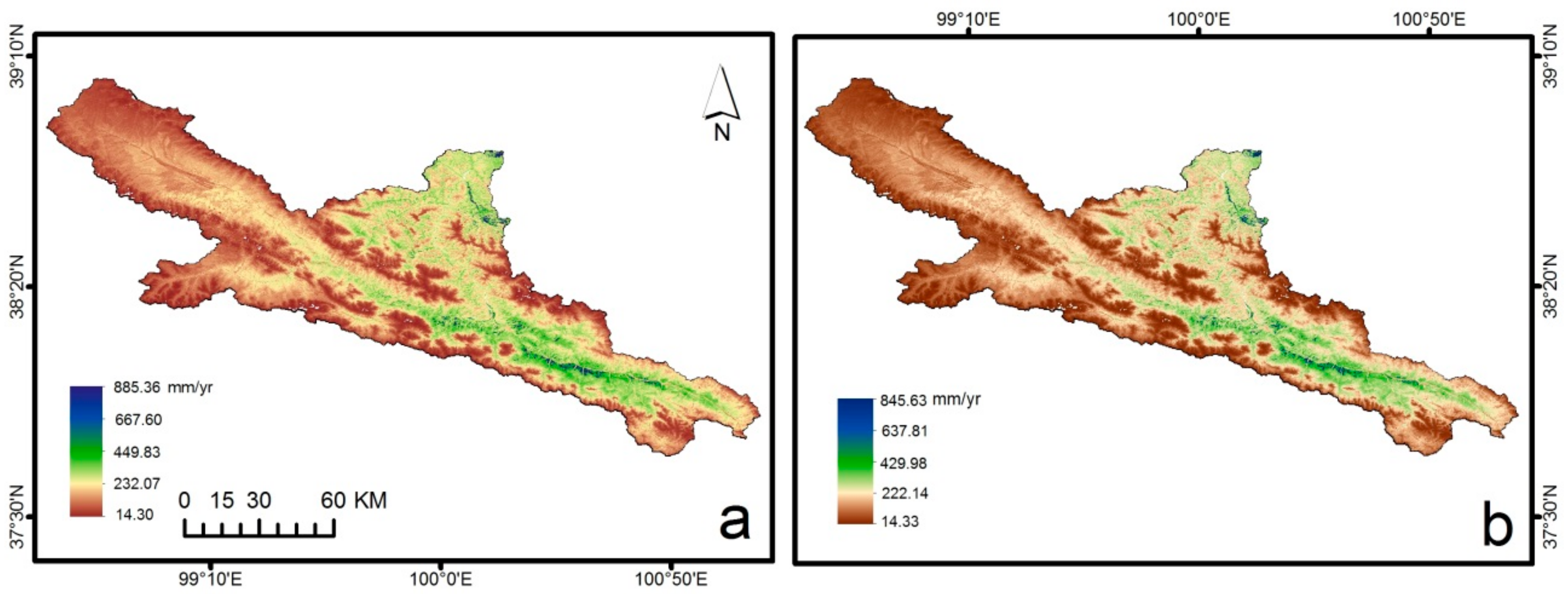
The findings of the simulation showed that the annual ET of the Upper Heihe watershed was around from 14.3 to 885 mm in two study years (Figure 8). Theoretically, the differences in ecophysiological properties (e.g., gsmax, Ω and vegetation height) between vegetation functional types might highly govern the ET losses distribution through their effects of transpirational loss [45]. At the same time, the architectures of different vegetation canopies would affect the over/understory radiation transfer mechanisms [46]. However, spatial heterogeneity of annual total ET had a huge diversity even within the same vegetation stand in the Upper Heihe watershed. The spatial average values of annual ET in deciduous and conifer stands had little discrepancy (131–145 mm) in both years. Annual potential ET losses in the watershed were much more reliant upon soil texture, topography and LAI distribution.
In terms of three major soil textures in Upper Heihe, the annual average modeled ET of silt loam was 340 mm in 2013 and 320 mm in 2014. For loam, it was 237 mm in 2013 and 219 mm in 2014, while clay only had average values of 162 mm in 2013 and 147 mm in 2014 even if it was the most widely distributed soil type in the watershed. One reason for the minimum ET loss of clay was because it had a lower vertical hydraulic conductivity that restricted the water infiltration from soil surface and further limited vegetation transpiration rate. And from HWSD, soil depth of clay was much shallower than that of others. As a result, under the same amount of water input, the rhizosphere of clay was more likely to be located in the saturated zone in the modeling domain. This could cause a lower ET efficiency because the transpirational losses in the saturated zone are much lower than that in unsaturated zone, as shown in Figure 7.
Additionally, annual ET was also highly in concordance with the DEM and LAI distributions in the simulation. Savenije [47] pointed out that topography is one of the most important factors affecting hydrological behavior in watershed scale, and closely related with distribution of plant functional types, soil properties and climate factors. The watershed with a relatively higher ET loss (>200 mm) is mainly concentrated in the south-eastern part of the watershed and near the river outlet area, which has a relatively lower altitude and gentle slope. Comparing with a high elevation mountainous area, the climate of a lower and outlet contiguous area was much warmer and wetter. However, it is important to note that the spatial distribution of soil texture and LAI were obtained from 1 km datasets. Although they were upscaled to 100 m to fit the model, they cannot provide such detailed spatial information. Considering the high dependence of ET on these two variables, the coarse spatial datasets might lead to unrealistic driving forces to some extent. For instance, the inaccurate classification of clay might over/underestimate total ET because of its restricted effect on vegetation transpiration.

3.3. Spatial-Temporal Patterns of GPP

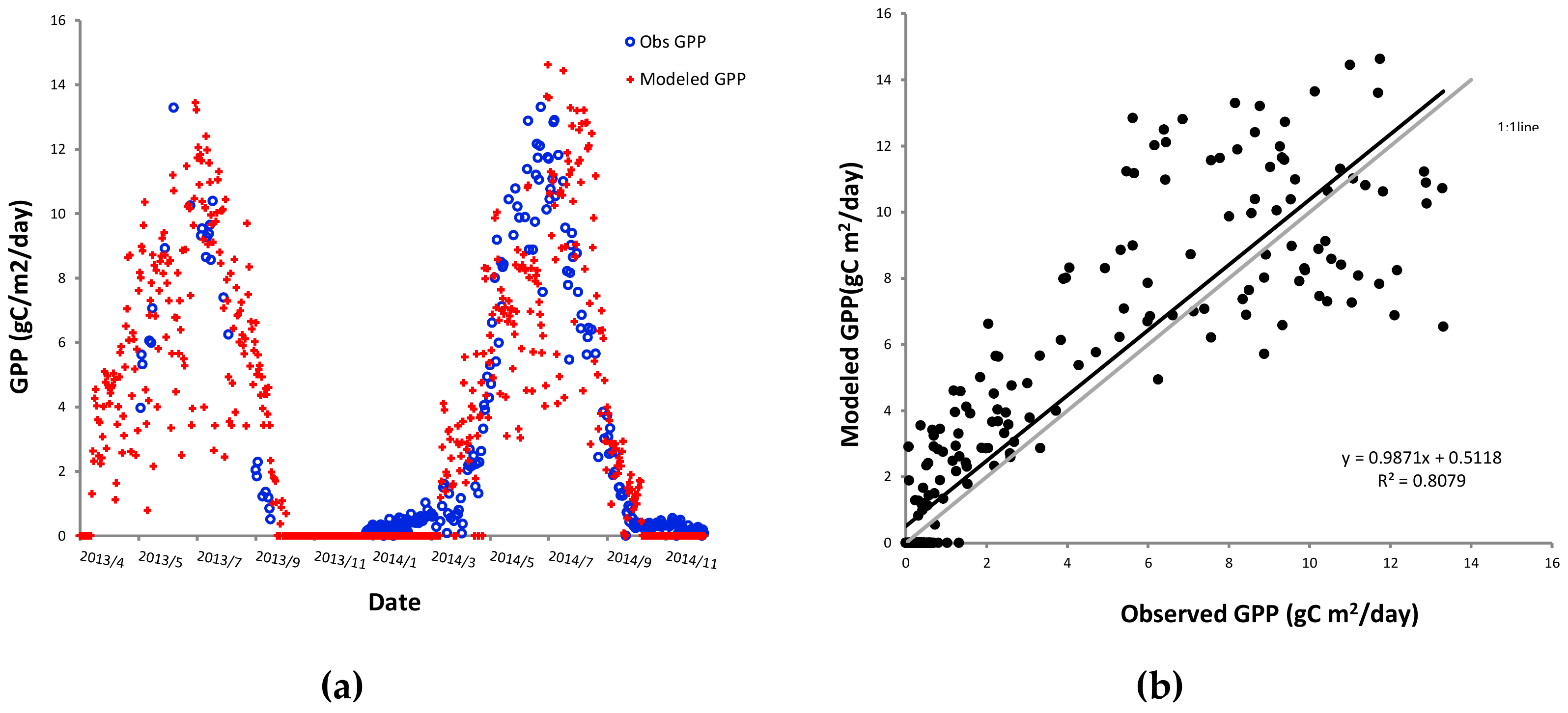
Figure 9 reveals the comparison between simulated and observed daily GPP at the Arou footprint site in 2013 and 2014. The model fairly captured seasonal variations of GPP and explained 71% with RMSE = 5.25 gC/m2/day in 2013 and 81% with 3.38 gC/m2/day in 2014. The model had a good performance in the estimation in GPP magnitudes of two study years. Nevertheless, comparing with measurements, there was a general overestimated GPP in spring and autumn while during June and July there was an underestimation in both years. Li [6] explored the spatiotemporal variations of water use efficiency (WUE), which represents the ratio of CO2 assimilation to vegetation transpiration [48] in the Heihe River Basin, and pointed that especially in the upper watershed, summer has the highest value of WUE, which is around 1.0–1.2 gC/mm/H2O/m2 comparing with the other seasons (0–0.4 gC/mm/H2O/m2). It validated temporal congruency between ET and GPP in the underestimated summer period when the melting runoff was possibly underestimated. From Figure 8b we can see there was a general overestimation of GPP within two years’ estimation. This discrepancy might be mainly attributed to the inexact representation of vegetation physiological characteristics consequent on the soil moisture statuses. As discussed above, due to the lack of simulating the soil freezing–thawing process, the model treated each soil texture in the watershed with constant hydraulic properties and remained in the optimal soil moisture condition whole year round. It triggered an overestimated GPP through two major reasons. One is the unrealistic higher stomatal conductance which would speed up photosynthetic process [49]. According to the Jarvis algorithm [50] embedded in DLM-Ecohydro, VSWC has a positive relationship with plant stomatal conductance when it is between the field capacity and permanent wilting point. Actually, for both frozen and thawing period, the infiltrated rate would not be as high as the model representation and quite a number of precipitation or snow melting water probably concentrate on the soil surface and drain out as lateral water fluxes, which would contribute to an increase in soil surface evaporation. This might explain why there was rare overestimation for simulated total ET although it is under the same gs as the GPP calculation. The experiment from Sonnentag [51] also manifested that compared with GPP, there was less sensitivity for ET in different soil moisture conditions. Another possible reason for the bias of modeled GPP was an inaccurate representation of ecosystem nitrogen (N) availability. Via the overestimation of gs, the model exaggerated local photosynthesis, which would raise the soil respiration and soil carbon decomposition and further created a conducive status for increasing biomass and N mineralization. It synergistically promoted photosynthesis and constituted a regional feedback mechanism [52,53,54]. On the other hand, the overestimated soil moisture also positively affected the leaf N content and further overstated GPP through the increased maximum carboxylation rate [55].
The simulated GPP was between 0 and 2119 gC m2/year in 2013 and from 0 to 2174 gC m2/year in 2014 (Figure 10). Generally, the location near a stream had a higher annual photosynthetic efficiency and the highest GPP were assembled in the north-eastern part of the Upper Heihe watershed where the terrain is flatter. And the location with higher elevation (higher than 3900 m a.s.l.) in the north-western and central part had the lowest efficiency of photosynthesis for both years.
The photosynthetic efficiency highly depended on the biophysical characters of different plant function types. From the simulated presentation, deciduous stands had a higher average annual GPP (482.81 gC m2/year in 2013 and 455.79 gC m2/year in 2014) compared to conifer forests (363.01 gC m2/year in 2013 and 343.11 gC m2/year in 2014) even if the distribution of conifer stands were mainly located in the outlet of the watershed with lower altitude, warmer climate and more adequate soil water resource. That is because deciduous stands had a higher stomatal conductance (gs,max = 5mm/s) and leaf N content (Nmax = 1.8%) than that of conifers (gs,max = 1.6mm/s; Nmax = 1.6%). Additionally, conifer canopy was more densely clumped than deciduous stands, with a clumping index of 0.5 and 0.8, respectively. It would decrease the ratio of sunlit leaves in the conifer canopy. Grassland had the most wide distribution within the Upper Heihe and also had the most spatially heterogeneous annual GPP, which ranged from 1.76 to 2119.18 gC m2/year in 2013 and 1.75 to 2174.46 gC m2/year in 2014. The spatial variability of grassland GPP had a high congruency with LAI, which reveals that the leaf abundance also took a significant contribution of grass photosynthetic efficiency, because it controlled vegetation surface energy balance through the interception of water and solar energy.
The distribution of GPP depended on complex interaction effects between topographic conditions, plant function types, vegetation biomass, regional meteorology, soil moisture, temperature and N dynamics in the model. The quantitative relationships and feedbacks between these spatial factors should be further explored. Theoretically, the model could run at any spatial resolution depending on the input dataset availability, while the lack of high-resolution soil types and LAI limited the ability of spatial patterns simulation. To fit the fusion of multi-source datasets, the spatial downscaling of DEM and land cover from 30 m to 100 m would also damage the original data qualities and further decrease the ability of model to explain GPP distribution due to the high correlation between these two factors and photosynthesis.

3.4. Co-Drive Mechanism of Ecosystem ET and GPP

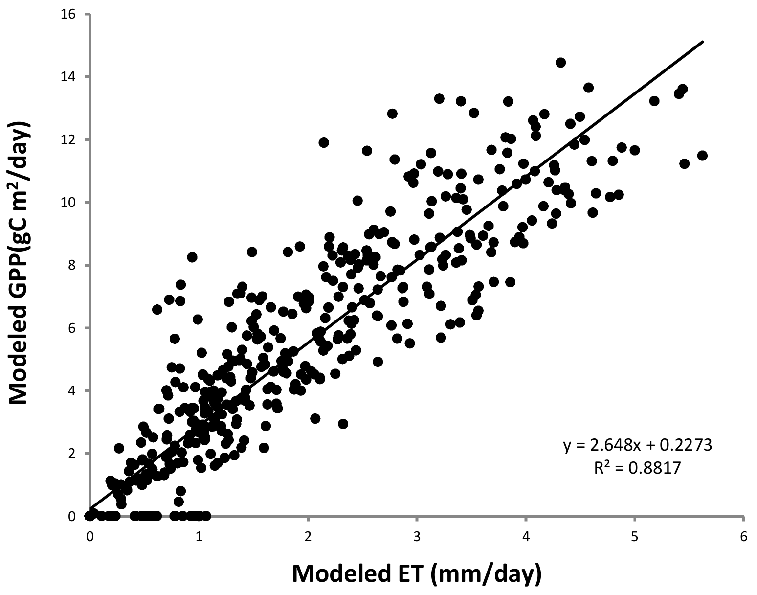
According to the above research we found that there is a strong synchronism between ecosystem evapotranspiration and photosynthesis. Figure 11 illustrates that the simulated ET and GPP have a significant positive liner relation (R2 = 0.88) within two study years. Except for a consistent seasonal variation with a same peak period at July and August, they also have a similar spatial heterogeneity. Previous research also pointed the consistent diurnal variation between ecosystem water and carbon fluxes [56], and Steduto [57] found that the annual accumulated carbon assimilation and evapotranspiration have a stable linear relationship. Except for the impact of soil moisture, another major reason is probably because the driving energies of ecosystem C–water cycle have a synchronous change. Canopy intercepted net radiation for ET and short-wave radiation for photosynthesis have a similar co-linear relation with input solar radiation. Additionally, as a common organ for transpiration and photosynthesis, the growth of leaves synchronously controls canopy ET and GPP fluctuation and this control is hardly affected by soil water and fertilizer conditions [58]. It also explains the similar spatial distribution between C–water fluxes and regional LAI discussed above. Furthermore, daily temperature and wind speed can also synchronously affect the exchange rate of CO2 and H2O between vegetation and the atmosphere through the control of enzymatic activity, stomatal conductance and vaporizing rate.

4. Conclusions

Based on two fundamental ecophysiological indicators, ET and GPP, this study utilized the DLM-Ecohydro model to simulate the exchanges between energy, water and carbon assimilation in the Upper Heihe watershed with a tightly coupled manner. The combination of in situ measurements and remotely sensed datasets provided detailed environmental disturbances from both nature and human beings, contributing a regionally accurate and spatially explicit simulation. The land surface model fully took topographical influence into consideration, modeling the lateral hydrological processes by solving a water balance equation. In order to accurately represent the ecophysiological processes in the watershed, the model separately simulated sunlit and shaded leaves and flexibly derived soil profiles as multiple layers according to the moisture regimes.
The simulation suggested that in spatial and temporal patterns, ET and GPP have significantly synchronous variations in the Upper Heihe watershed. Although the precipitation was mainly concentrated during May and September in the watershed, soil water content was still a major limiting factor for vegetation transpiration and photosynthesis efficiency in mid-summer. The spatial distribution of ET highly depends on soil texture. Silt loam and clay had the maximum and minimum annual ET loss, respectively, mainly because of their different abilities of hydraulic conductance. Vegetation transpiration accounted for the most part of ecosystem ET losses in the two study years. Photosynthesis was more sensitive to plant functional types: Deciduous forests had the highest annual carbon assimilation rate owing to it having a higher stomatal conductance and leaf nitrogen content and a lower canopy clumping index. LAI and topography, however, made a strong contribution for both ecophysiological processes simultaneously.
There are also some limitations of this study. Because the model did not consider the dynamics of frozen soil and the melting runoff from glaciers in the alpine regions, it would cause an unreality estimation of soil moisture regimes during the frozen and major melting seasons. While overall, the model showed a fair performance for the simulation of hydro-ecological processes, especially during vegetation growing seasons.

Author Contributions

Conceptualization, B.C.; data curation, H.J., S.S. and X.L.; formal analysis, H.J., S.S., S.M., X.L. and L.G.; funding acquisition, B.C.; investigation, H.J., S.S.; methodology, B.C., H.J., S.S., H.Z. and S.M.; project administration, B.C.; resources, B.C.; software, H.J., S.S. and H.Z.; supervision, B.C.; validation, H.J., S.S. and L.G.; visualization, H.J., S.S. and L.G.; writing – original draft, H.J.; and writing – review and editing, B.C. and S.S.

Funding

This research was funded by the National Key R&D Program of China (2018YFA0606001, 2017YFA0604301, 2017YFA0604302, 2017YFC0503904), an international partnership program of Chinese Academy of Sciences (Grant #131A11KYSB20170025), a research project funded by the State Key Laboratory of Resources and Environmental Information System (O88RA901YA, O8R8A085YA) and a project funded by the National Natural Science Foundation of China (41771114).

Acknowledgments

We thank the Heihe Watershed Allied Telemetry Experimental Research (HiWATER) program for providing the ecophysiological validation of datasets of the Arou station in the Upper Heihe watershed.

Conflicts of Interest

The authors declare no conflict of interest. The funders had no role in the design of the study; in the collection, analyses, or interpretation of data; in the writing of the manuscript, or in the decision to publish the results.

References

  1. Chen, B.; Chen, J.M.; Ju, W. Remote sensing-based ecosystem-atmosphere simulation scheme (EASS)—Model formulation and test with multiple-year data. Ecol. Model. 2007, 209, 277–300. [Google Scholar] [CrossRef]
  2. Govind, A.; Cowling, S.; Kumari, J.; Rajan, N.; Al-Yaari, A. Distributed modeling of ecohydrological processes at high spatial resolution over a landscape having patches of managed forest stands and crop fields in SW Europe. Ecol. Model. 2015, 297, 126–140. [Google Scholar] [CrossRef]
  3. Govind, A.; Kumari, J. Understanding the Terrestrial Carbon Cycle: An Ecohydrological Perspective. Int. J. Ecol. 2014, 2014, 712537. [Google Scholar] [CrossRef]
  4. Biederman, J.A.; Scott, R.L.; Goulden, M.L.; Vargas, R.; Litvak, M.E.; Kolb, T.E.; Yepez, E.A.; Oechel, W.C.; Blanken, P.D.; Bell, T.W.; et al. Terrestrial carbon balance in a drier world: The effects of water availability in southwestern North America. Glob. Chang. Biol. 2016, 22, 1867–1879. [Google Scholar] [CrossRef] [PubMed]
  5. Gea-Izquierdo, G.; Guibal, F.; Joffre, R.; Ourcival, J.M.; Simioni, G.; Guiot, J. Modelling the climatic drivers determining photosynthesis and carbon allocation in evergreen Mediterranean forests using multiproxy long time series. Biogeosciences 2015, 12, 3695–3712. [Google Scholar] [CrossRef] [Green Version]
  6. LU, L.; LI, X.; HUANG, C.; Frank, V. Analysis of the Spatio-Temporal Characteristics of Water Use Efficiency of Vegetation in West China. J. Glaciol. Geocryol. 2007, 29, 777–784. [Google Scholar]
  7. Wang, P.; Qiu, J.; Huo, Z.; Anderson, M.; Zhou, Y.; Bai, Y.; Liu, T.; Ren, S.; Feng, R.; Chen, P. Temporal Downscaling of Crop Coefficients for Winter Wheat in the North China Plain: A Case Study at the Gucheng Agro-Meteorological Experimental Station. Water 2017, 9, 155. [Google Scholar] [CrossRef]
  8. Richardson, A.D.; Anderson, R.S.; Arain, M.A.; Barr, A.G.; Bohrer, G.; Chen, G.; Chen, J.M.; Ciais, P.; Davis, K.J.; Desai, A.R.; et al. Terrestrial biosphere models need better representation of vegetation phenology: Results from the North American Carbon Program Site Synthesis. Glob. Chang. Biol. 2012, 18, 566–584. [Google Scholar] [CrossRef]
  9. Rodríguez, N.C.; Melgarejo, L.M.; Blair, M.W. Purple Passion Fruit, Passiflora edulis Sims f. edulis, Variability for Photosynthetic and Physiological Adaptation in Contrasting Environments. Agronomy 2019, 9, 231. [Google Scholar] [CrossRef]
  10. Gennaretti, F.; Gea-Izquierdo, G.; Boucher, E.; Berninger, F.; Arseneault, D.; Guiot, J. Ecophysiological modeling of photosynthesis and carbon allocation to the tree stem in the boreal forest. Biogeosciences 2017, 14, 4851–4866. [Google Scholar] [CrossRef] [Green Version]
  11. Nadal-Sala, D.; Keenan, T.F.; Sabaté, S.; Gracia, C. Forest Eco-Physiological Models: Water Use and Carbon Sequestration. In Managing Forest Ecosystems: The Challenge of Climate Change; Bravo, F., LeMay, V., Jandl, R., Eds.; Springer: Dordrecht, The Netherlands, 2017; pp. 81–102. [Google Scholar]
  12. Li, L.; Wang, Y.; Arora, V.K.; Eamus, D.; Shi, H.; Li, J.; Cheng, L.; Cleverly, J.; Hajima, T.; Ji, D.; et al. Evaluating Global Land Surface Models in CMIP5: Analysis of Ecosystem Water- and Light-Use Efficiencies and Rainfall Partitioning. J. Clim. 2018, 31, 2995–3008. [Google Scholar] [CrossRef]
  13. Baldocchi, D.D.; Wilson, K.B. Modeling CO2 and water vapor exchange of a temperate broadleaved forest across hourly to decadal time scales. Ecol. Model. 2001, 142, 155–184. [Google Scholar] [CrossRef]
  14. Emanuel, R.E.; Epstein, H.E.; McGlynn, B.L.; Welsch, D.L.; Muth, D.J.; D’Odorico, P. Spatial and temporal controls on watershed ecohydrology in the northern Rocky Mountains. Water Resour. Res. 2010, 46. [Google Scholar] [CrossRef]
  15. Govind, A.; Chen, J.M.; Margolis, H.; Ju, W.; Sonnentag, O.; Giasson, M. A spatially explicit hydro-ecological modeling framework (BEPS-TerrainLab V2.0): Model description and test in a boreal ecosystem in Eastern North America. J. Hydrol. 2009, 367, 200–216. [Google Scholar] [CrossRef]
  16. Sonnentag, O.; Talbot, J.; Chen, J.M.; Roulet, N.T. Using direct and indirect measurements of leaf area index to characterize the shrub canopy in an ombrotrophic peatland. Agric. For. Meteorol. 2007, 144, 200–212. [Google Scholar] [CrossRef]
  17. Zhengkun, Z.; Guangcan, Z.; Shunsheng, L.; Bin, P.; Zhiqiang, X.; Ping, X.; Xia, L. Effects of soil moisture on photosynthesis diurnal changes of Prunus sibirica L. Sci. Soil Water Conserv. 2012, 10, 99–104. [Google Scholar]
  18. Liu, Z.H.; McVicar, T.R.; Li, L.T.; Van Niel, T.G.; Yang, Q.K.; Li, R.; Mu, X.M. Modeling spatial distribution of pan evaporation based on quinat-variate thin plate spline function. Sci. Soil Water Conserv. 2006, 4, 23–30. [Google Scholar]
  19. Dang, S.Z.; Liu, C.M.; Wang, Z.G.; Wu, M.Y. Analyses on temporal variations of snowmelt runoff time in the upper reaches of Heihe River and its climate causes. J. Glaciol. Geocryol. 2012, 34, 920–926. [Google Scholar]
  20. Yan, M.; Li, Z.Y.; Tian, X.; Chen, E.X.; Gu, C.Y. Remote sensing estimation of gross primary productivity and its response to climate change in the upstream of Heihe River Basin. Chin. J. Plant Ecol. 2016, 40, 1–12. [Google Scholar]
  21. Shang, X.; Jiang, X.; Jia, R.; Wei, C. Land Use and Climate Change Effects on Surface Runoff Variations in the Upper Heihe River Basin. Water 2019, 11, 344. [Google Scholar] [CrossRef]
  22. Bi, L.M.; Hou, H.Y.; Yang, L.F. Analysis on change trend of runoff in Yingluoxia station of Heihe River. Yellow River 2013, 35, 23–25. [Google Scholar]
  23. Wang, R.; Cheng, Q.; Liu, L.; Yan, C.; Huang, G. Multi-Model Projections of Climate Change in Different RCP Scenarios in an Arid Inland Region, Northwest China. Water 2019, 11, 347. [Google Scholar] [CrossRef]
  24. Yang, Y.; Chen, R.; Han, C.; Qing, W. Measurement and estimation of the summertime daily evapotranspiration on alpine meadow in the Qilian Mountains, northwest China. Environ. Earth Sci. 2013, 68, 2253–2261. [Google Scholar] [CrossRef]
  25. Wang, Y. Remote Estimation of Carbon Fluxes and Carbon Sequestration Capacity over Cropland Based on Eddy Covariance Observation. Master’s Thesis, Henan Polytechnic University, Heinan Province, China, 2015. [Google Scholar]
  26. Sun, S.; Chen, B.; Ge, M.; Qu, J.; Che, T.; Zhang, H.; Lin, X.; Che, M.; Zhou, Z.; Guo, L.; et al. Improving soil organic carbon parameterization of land surface model for cold regions in the Northeastern Tibetan Plateau, China. Ecol. Model. 2016, 330, 1–15. [Google Scholar] [CrossRef] [Green Version]
  27. Wang, Y.H.; Yang, D.W.; Lei, H.M.; Yang, H. Impact of cryosphere hydrological processes on the river runoff in the upper reaches of Heihe River. J. Hydraul. Eng. 2015, 46, 1064–1071. [Google Scholar]
  28. Qin, J.; Ding, Y.; Wu, J.; Gao, M.; Yi, S.; Zhao, C.; Ye, B.; Li, M.; Wang, S. Understanding the impact of mountain landscapes on water balance in the upper Heihe River watershed in northwestern China. J. Arid Land 2013, 5, 366–383. [Google Scholar] [CrossRef] [Green Version]
  29. Lu, L.; Li, X.; Cheng, G.D. Landscape evolution in the middle Heihe River Basin of north-west China during the last decade. J. Arid Environ. 2003, 53, 395–408. [Google Scholar] [CrossRef] [Green Version]
  30. Chen, J.; Chen, B.; Black, T.A.; Innes, J.L.; Wang, G.; Kiely, G.; Hirano, T.; Wohlfahrt, G. Comparison of terrestrial evapotranspiration estimates using the mass transfer and Penman-Monteith equations in land surface models. J. Geophys. Res. Biogeosci. 2013, 118, 1715–1731. [Google Scholar] [CrossRef]
  31. Farquhar, G.D.; von Caemmerer, S.V.; Berry, J.A. A Biochemical Model of Photosynthetic CO2 Assimilation in Leaves of C3 Species. Planta 1980, 149, 78–90. [Google Scholar] [CrossRef]
  32. GALE, M.R.; GRIGAL, D.F. Vertical root distributions of northern tree species in relation to successional status. Can. J. For. Res. 1987, 17, 829–834. [Google Scholar] [CrossRef]
  33. Voinov, A.A.; Fitz, H.C.; Costanza, R. Surface water flow in landscape models: 1. Everglades case study. Ecol. Model. 1998, 108, 131–144. [Google Scholar] [CrossRef]
  34. Govind, A.; Chen, J.M.; McDonnell, J.; Kumari, J.; Sonnentag, O. Effects of lateral hydrological processes on photosynthesis and evapotranspiration in a boreal ecosystem. Ecohydrology 2011, 4, 394–410. [Google Scholar] [CrossRef]
  35. Oleson, K.W.; Lawrence, D.M.; Gordon, B.; Flanner, M.G.; Kluzek, E.; Peter, J.; Levis, S.; Swenson, S.C.; Thornton, E.; Feddema, J. Technical Description of Version 4.0 of the Community Land Model (CLM); NCAR Technical Note, NCAR/TN-478+STR; National Center for Atmospheric Research: Boulder, CO, USA, 2010. [Google Scholar]
  36. Li, X.; Cheng, G.; Liu, S.; Xiao, Q.; Ma, M.; Jin, R.; Che, T.; Liu, Q.; Wang, W.; Qi, Y.; et al. Heihe Watershed Allied Telemetry Experimental Research (HiWATER): Scientific Objectives and Experimental Design. Bull. Am. Meteorol. Soc. 2013, 94, 1145–1160. [Google Scholar] [CrossRef]
  37. Liu, S.M.; Xu, Z.W.; Wang, W.Z.; Jia, Z.Z.; Zhu, M.J.; Bai, J.; Wang, J.M. A comparison of eddy-covariance and large aperture scintillometer measurements with respect to the energy balance closure problem. Hydrol. Earth Syst. Sci. 2011, 15, 1291–1306. [Google Scholar] [CrossRef] [Green Version]
  38. Liu, S.; Li, X.; Xu, Z.; Che, T.; Xiao, Q.; Ma, M.; Liu, Q.; Jin, R.; Guo, J.; Wang, L.; et al. The Heihe Integrated Observatory Network: A Basin-Scale Land Surface Processes Observatory in China. Vadose Zone J. 2018, 17. [Google Scholar] [CrossRef]
  39. Lloyd, J.; Taylor, J.A. On the temperature dependence of soil respiration. Funct. Ecol. 1994, 8, 315–323. [Google Scholar] [CrossRef]
  40. Pan, X.; Li, X.; Cheng, G.; Chen, R.; Hsu, K. Impact Analysis of Climate Change on Snow over a Complex Mountainous Region Using Weather Research and Forecast Model (WRF) Simulation and Moderate Resolution Imaging Spectroradiometer Data (MODIS)-Terra Fractional Snow Cover Products. Remote Sens. 2017, 9, 774. [Google Scholar] [CrossRef]
  41. Molotch, N.P.; Blanken, P.D.; Williams, M.W.; Turnipseed, A.A.; Monson, R.K.; Margulis, S.A. Estimating sublimation of intercepted and sub-canopy snow using eddy covariance systems. Hydrol. Process. 2007, 21, 1567–1575. [Google Scholar] [CrossRef]
  42. Li, H.Y.; Wang, J. The snowmelt runoff model applied in the upper Heihe River Basin. J. Glaciol. Geocryol. 2008, 5, 769–775. [Google Scholar]
  43. Li, Q.; Chen, H.S. Variation of seasonal frozen soil in East China and their association with monsoon activity under the background of global warming. Clim. Chang. Res. Lett. 2013, 2, 47–53. [Google Scholar] [CrossRef]
  44. Schlesinger, W.H.; Jasechko, S. Transpiration in the global water cycle. Agric. For. Meteorol. 2014, 189, 115–117. [Google Scholar] [CrossRef]
  45. Wilson, K.B.; Baldocchi, D.D.; Hanson, P.J. Leaf age affects the seasonal pattern of photosynthetic capacityand net ecosystem exchange of carbon in a deciduous forest. Plant Cell Environ. 2001, 24, 571–583. [Google Scholar] [CrossRef]
  46. Garbulsky, M.F.; Penuelas, J.; Gamon, J.; Inoue, Y.; Filella, I. The photochemical reflectance index (PRI) and the remote sensing of leaf, canopy and ecosystem radiation use efficiencies: A review and meta-analysis. Remote Sens. Environ. 2011, 115, 281–297. [Google Scholar] [CrossRef]
  47. Savenije, H.H.G. HESS Opinions “Topography driven conceptual modelling (FLEX-Topo)”. Hydrol. Earth Syst. Sci. 2010, 14, 2681–2692. [Google Scholar] [CrossRef]
  48. Fischer, R.A.; Turner, N.C. Plant productivity in arid and semi-arid zones. Annu. Rev. Plant Physiol. 1978, 29, 277–317. [Google Scholar] [CrossRef]
  49. Chen, J.M.; Liu, J.; Cihlar, J.; Goulden, M.L. Daily canopy photosynthesis model through temporal and spatial scaling for remote sensing applications. Ecol. Model. 1999, 124, 99–119. [Google Scholar] [CrossRef] [Green Version]
  50. Jarvis, P.G. Interpretation of variations in leaf water potential and stomatal conductance found in canopies in field. Philos. Trans. R. Soc. Lond. Ser. B Biol. Sci. 1976, 273, 593–610. [Google Scholar] [CrossRef]
  51. Sonnentag, O.; Chen, J.M.; Roulet, N.T.; Ju, W.; Govind, A. Spatially explicit simulation of peatland hydrology and carbon dioxide exchange: Influence of mesoscale topography. J. Geophys. Res. Biogeosci. 2008, 113, G02005. [Google Scholar] [CrossRef]
  52. Tan, X.; Chang, S.X. Soil compaction and forest litter amendment affect carbon and net nitrogen mineralization in a boreal forest soil. Soil Tillage Res. 2007, 93, 77–86. [Google Scholar] [CrossRef]
  53. Traoré, S.; Thiombiano, L.; Millogo, J.R.; Guinko, S. Carbon and nitrogen enhancement in Cambisols and Vertisols by Acacia spp. in eastern Burkina Faso: Relation to soil respiration and microbial biomass. Appl. Soil Ecol. 2007, 35, 660–669. [Google Scholar]
  54. Govind, A.; Chen, J.M.; Ju, W. Spatially explicit simulation of hydrologically controlled carbon and nitrogen cycles and associated feedback mechanisms in a boreal ecosystem. J. Geophys. Res. Biogeosci. 2009, 114, G02006. [Google Scholar] [CrossRef]
  55. Arain, M.A.; Yuan, F.; Black, T.A. Soil–plant nitrogen cycling modulated carbon exchanges in a western temperate conifer forest in Canada. Agric. For. Meteorol. 2006, 140, 171–192. [Google Scholar] [CrossRef]
  56. Zhu, Z.; Sun, X.; Zhang, R.; Su, H.; Tang, X. Rapid measurements of CO2 flux density and water use efficiency of crop community. J. Appl. Ecol. 2004, 15, 1684–1686. [Google Scholar]
  57. Steduto, P.; Albrizio, R. Resource use efficiency of field-grown sunflower, sorghum, wheat and chickpea II. Water use efficiency and comparison with radiation use efficiency. Agric. For. Meteorol. 2005, 130, 269–281. [Google Scholar] [CrossRef]
  58. Yu, G.R.; Wang, Q.F.; Zhuang, J. Modeling the water use efficiency of soybean and maize plants under environmental stresses: Application of a synthetic model of photosynthesis-transpiration based on stomatal behavior. J. Plant Physiol. 2004, 161, 303–318. [Google Scholar] [CrossRef] [PubMed]
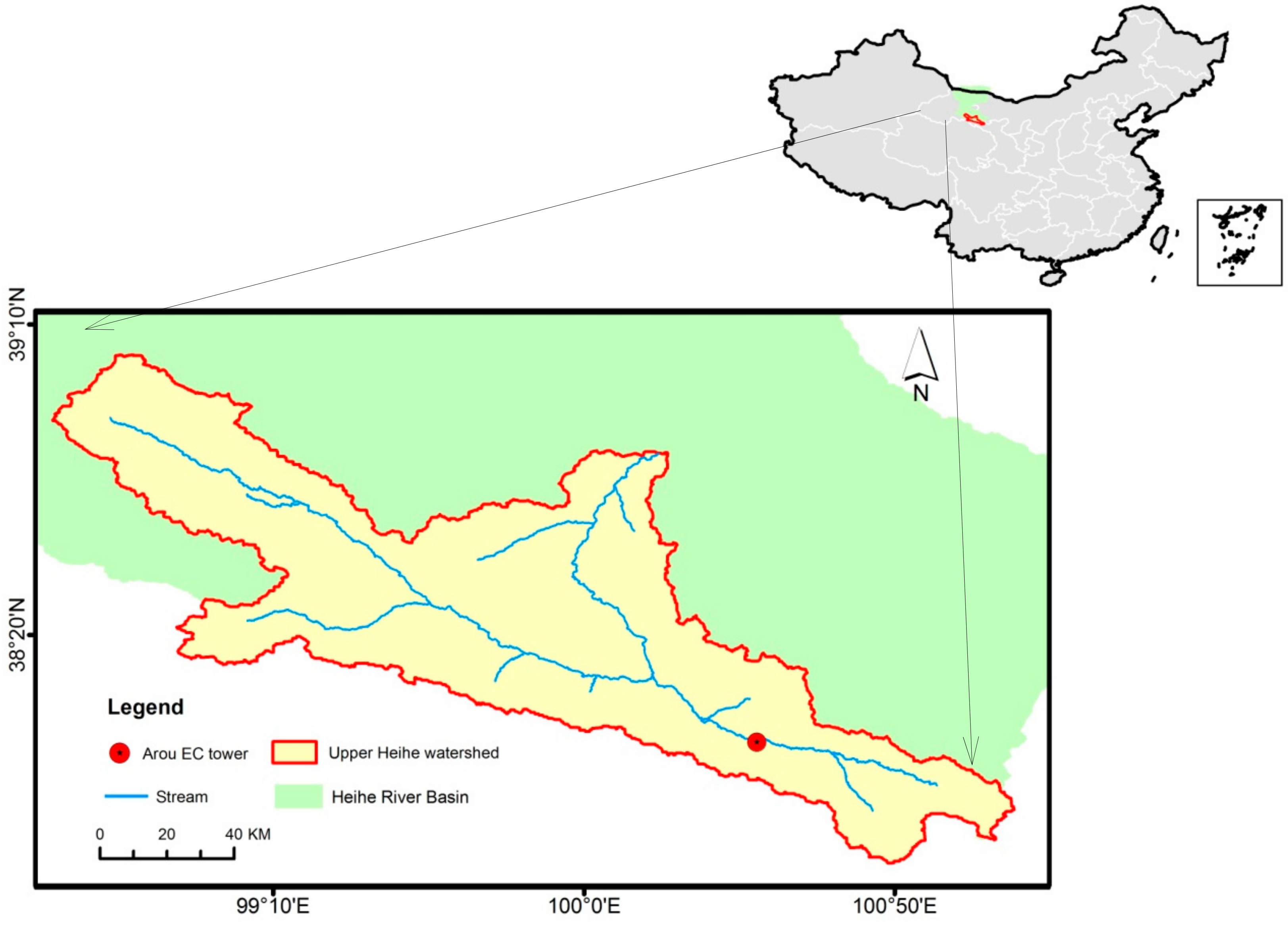
Figure 1. Location of the Upper Heihe watershed.
Water 11 01242 g001
Figure 2. Flow chart of the DLM-Ecohydro model.
Water 11 01242 g002
Figure 3. Main spatial dataset of the Upper Heihe watershed prepared for model input: (a) digital elevation model (DEM), (b) land cover, (c) soil texture, and (d) maximum leaf area index (LAI).
Water 11 01242 g003
Figure 4. Temporal dynamics of volumetric soil water content (VSWC) between day of the year (DOY) 170–300 in 2013 (a) and 2014 (b).
Water 11 01242 g004
Figure 5. Temporal dynamics of simulated subsurface baseflow (SSB) and surface overland flow (SOLF) and precipitation in 2013 and 2014 at Arou Station.
Water 11 01242 g005
Figure 6. (a) Time-series comparison of modeled and observed evapotranspiration (ET) for 2013 and 2014 in the Arou footprint area. (b) Combined comparison between simulated and measured ET for 2013 and 2014.
Water 11 01242 g006
Figure 7. Simulated magnitudes of ecosystem ET sub-components in the Arou footprint area in 2013 and 2014, between DOY 1 and 365.
Water 11 01242 g007
Figure 8. Simulated spatial patterns of annual total ET for 2013 (a) and 2014 (b) in the Upper Heihe watershed.
Water 11 01242 g008
Figure 9. (a) Time-series comparison of modeled and observed gross primary productivity (GPP) for 2013 and 2014 in the Arou footprint area. (b) Combined comparison between simulated and measured GPP for 2013 and 2014.
Water 11 01242 g009
Figure 10. Simulated spatial patterns of annual total GPP for 2013 (a) and 2014 (b) in the Upper Heihe watershed.
Water 11 01242 g010
Figure 11. The relationship between simulated ET and GPP in two study years.
Water 11 01242 g011
Table 1. Biophysical parameters of major landscape types in the Upper Heihe watershed.
Parameter NamesUnitConiferDeciduousGrasslandWetland
Canopy clumping index-0.50.80.90.9
Maximum stomatal conductance m/s0.00160.0050.00550.005
Root decay rate-0.940.960.950.93
Maximum carboxylation rate at 25 °Cµmol/m2/s33604033
Precipitation interception coefficientmm/LAI/day0.20.30.250.1
Max. leaf N content%1.61.81.61.2
Ration of gs,max of overstory to understory-1.70.51.21
Optimum temperature for photosynthesis°C20252020
Table 2. Hydraulic properties of four main soil types in the Upper Heihe watershed.
Soil Hydraulic ParameterUnitClayLoamClay LoamSandy Loam
Field capacity-0.40.270.30.23
Wilting point-0.270.120.20.1
Porosity%0.4570.4630.4640.453
Max. surface conductancemm/s0.20.80.51
Ksat,verm/day0.111.81.23.2
Ksat,horm/day102.51.53.5
Ks decay ratem−10.020.040.0290.042
The exponent of the Brokes–Corey parameter-11.45.395.54.9