Spatial Statistical Assessment of Groundwater PCE (Tetrachloroethylene) Diffuse Contamination in Urban Areas


 ,
,  and
and 
Abstract
1. Introduction
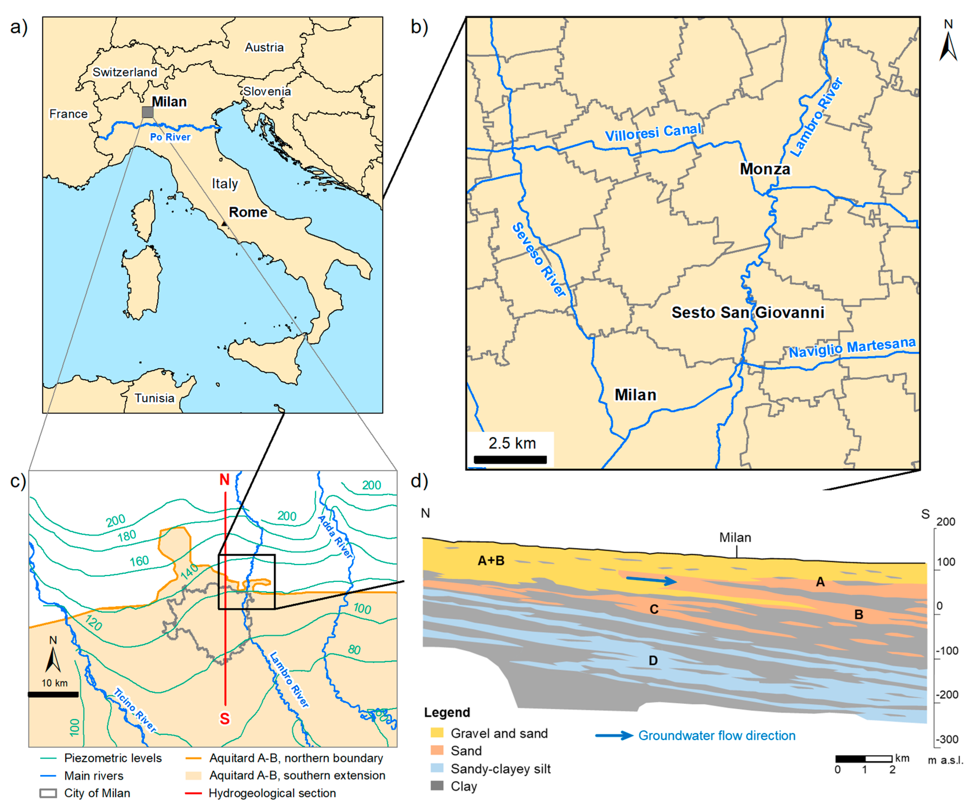
2. Study Area
3. Materials and Methods
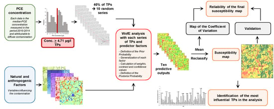
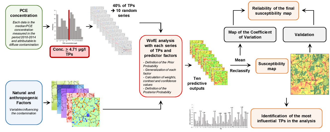
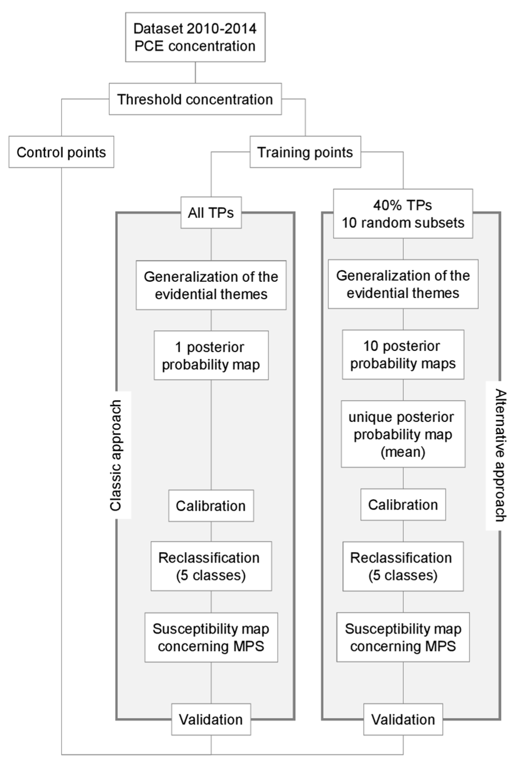
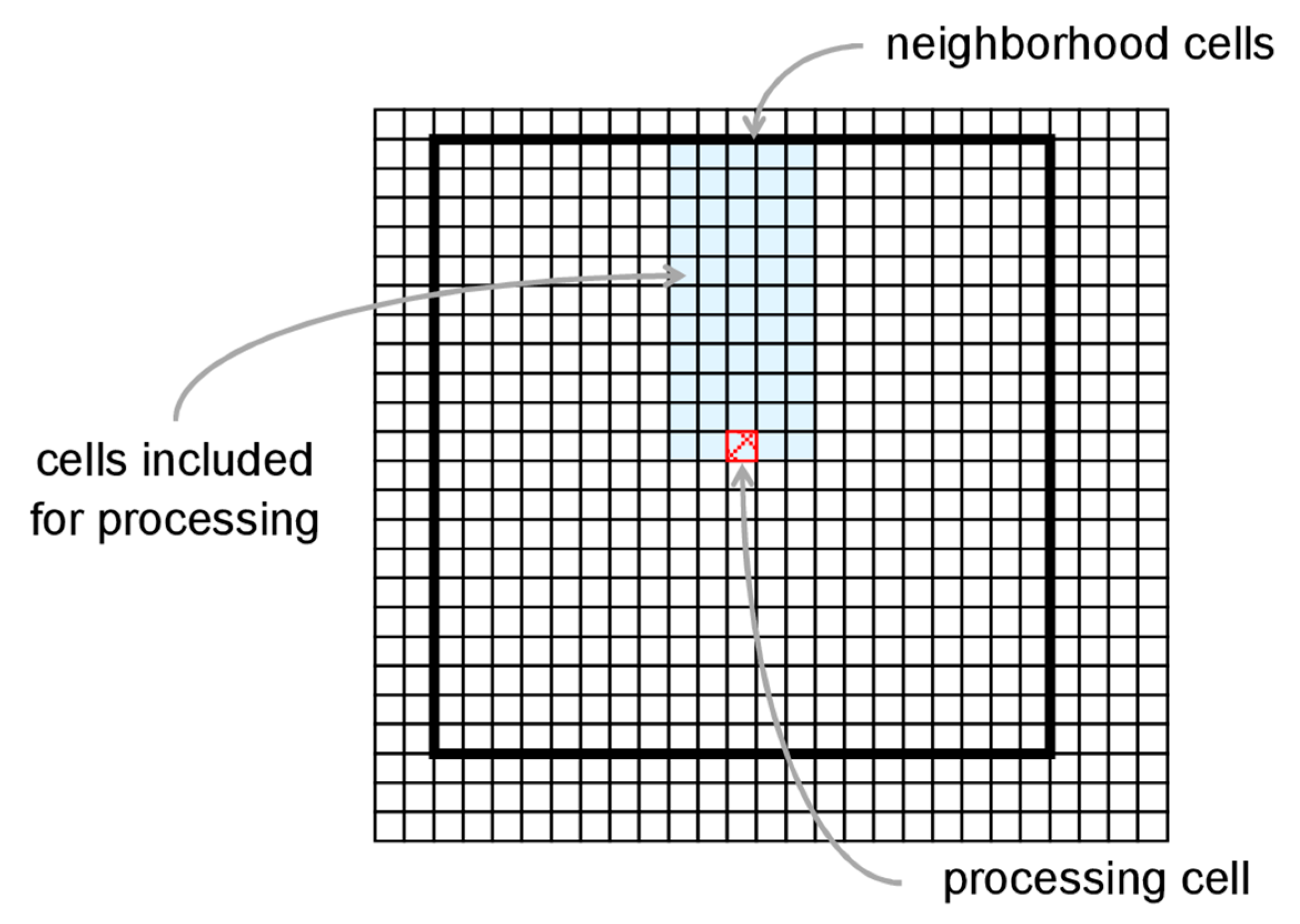
3.1. The WofE Modelling Technique: Classic and Alternative Approach
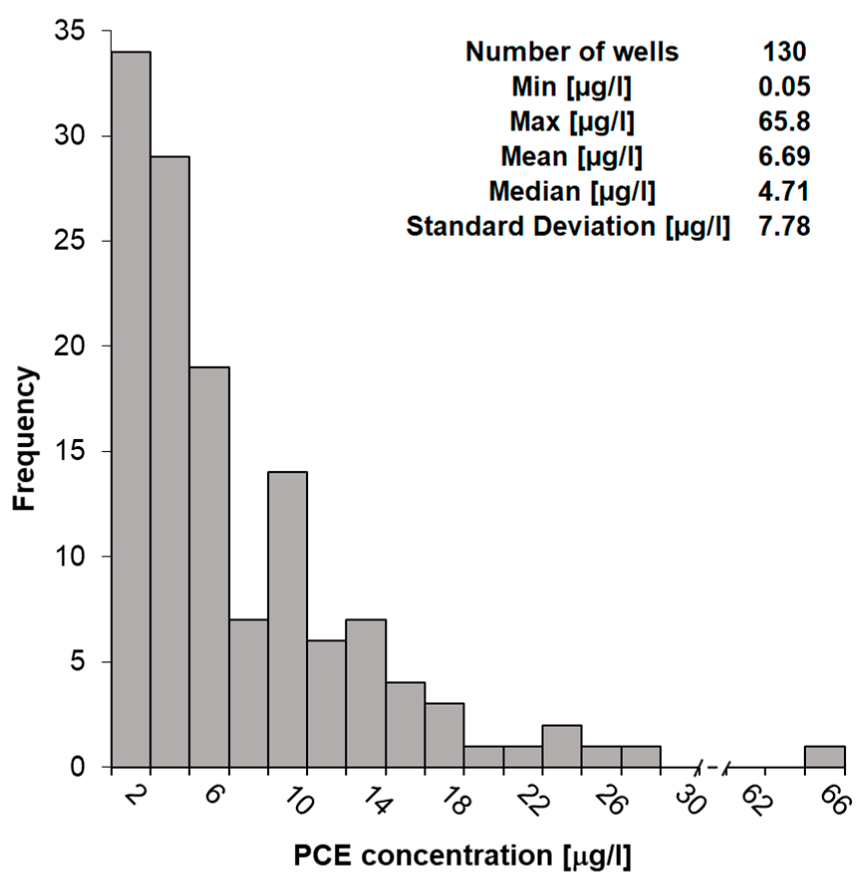
3.2. Training Points
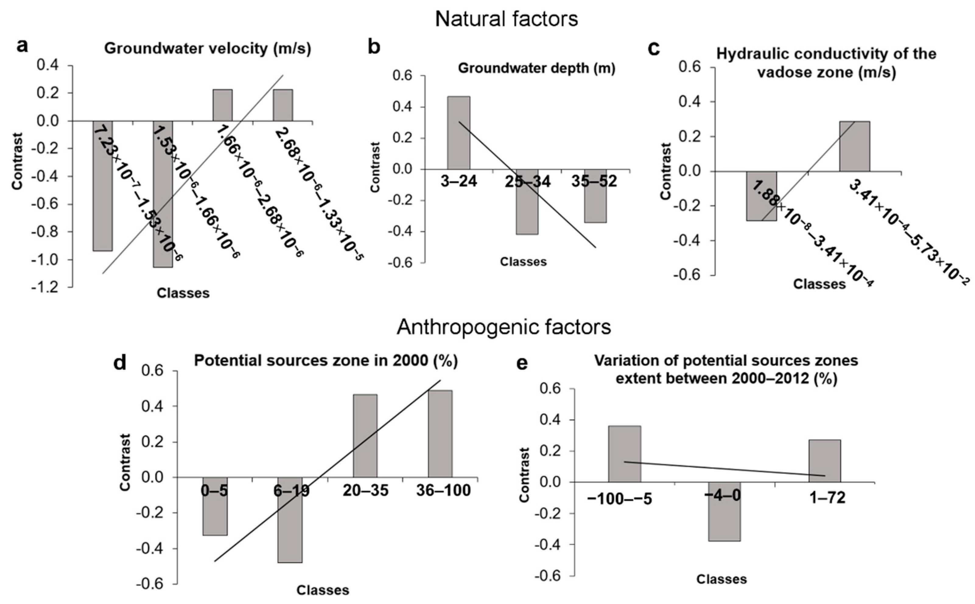
3.3. Evidential Themes
- groundwater depth,
- hydraulic conductivity of the vadose zone,
- groundwater velocity,
- percentage of “potential sources zone” (PSZ) extent in 2000, including industrial, artisanal, and commercial settlements,
- PSZ variation during the period 2000–2012.
4. Results
4.1. Contrasts of the Generalized Evidential Themes
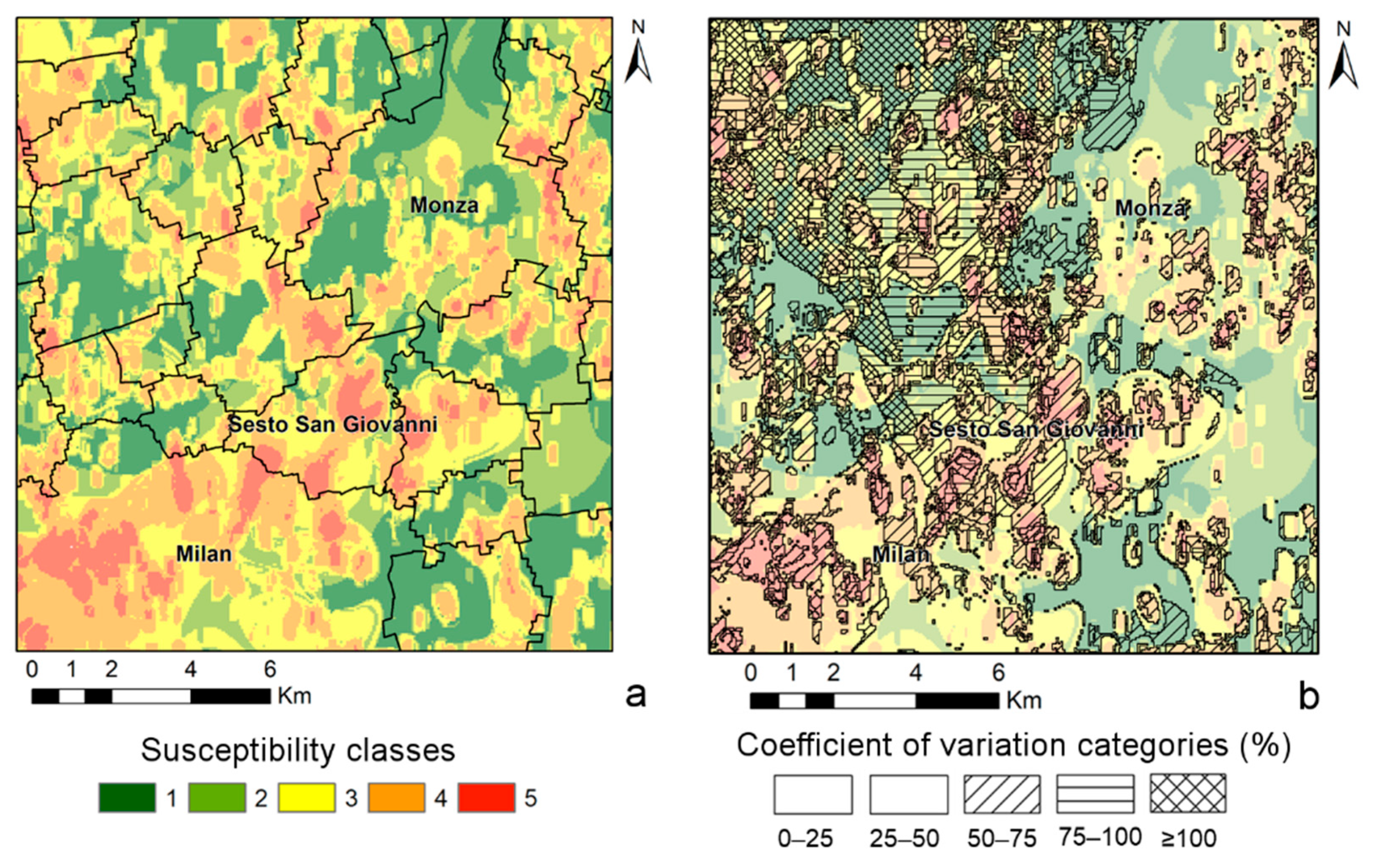
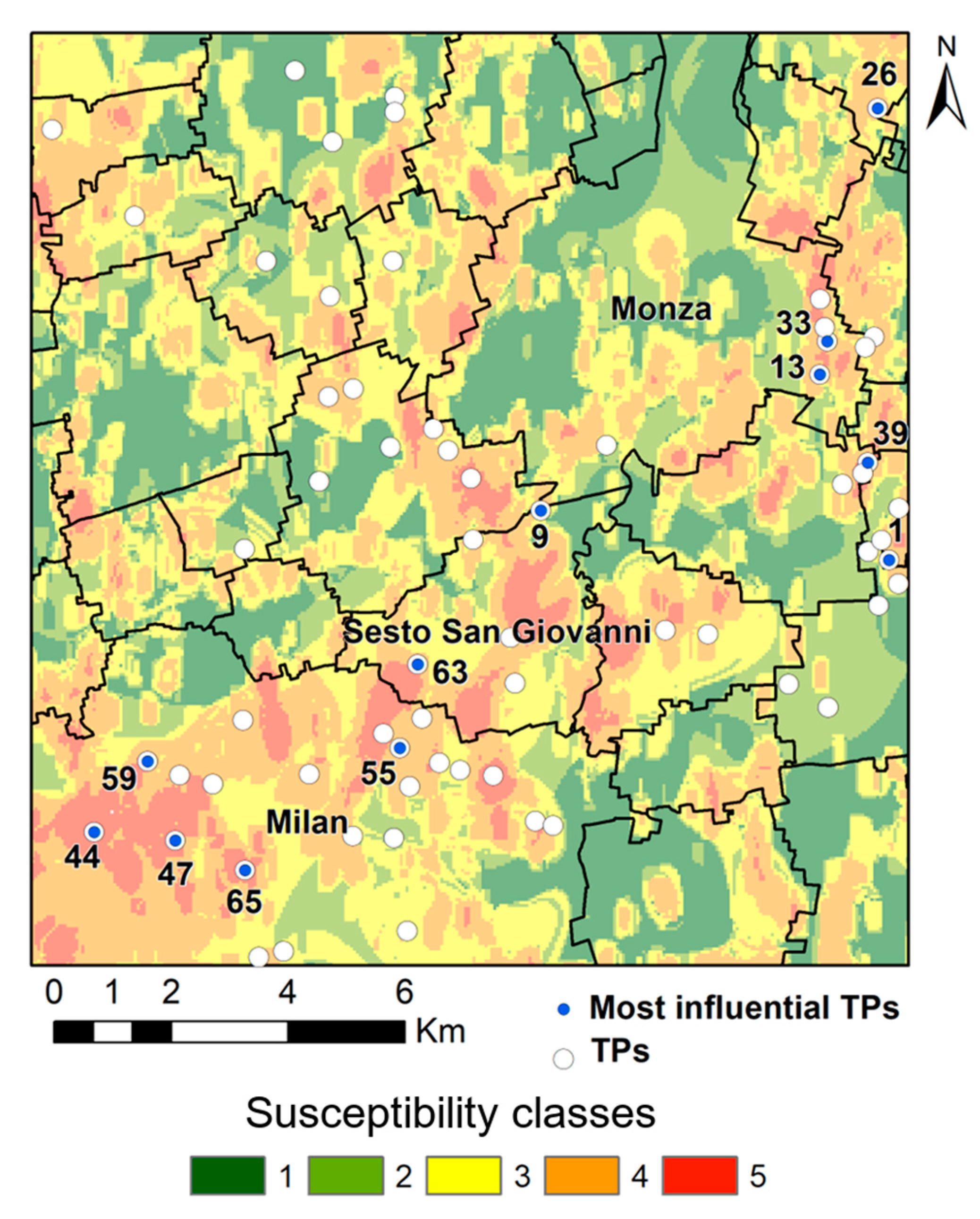
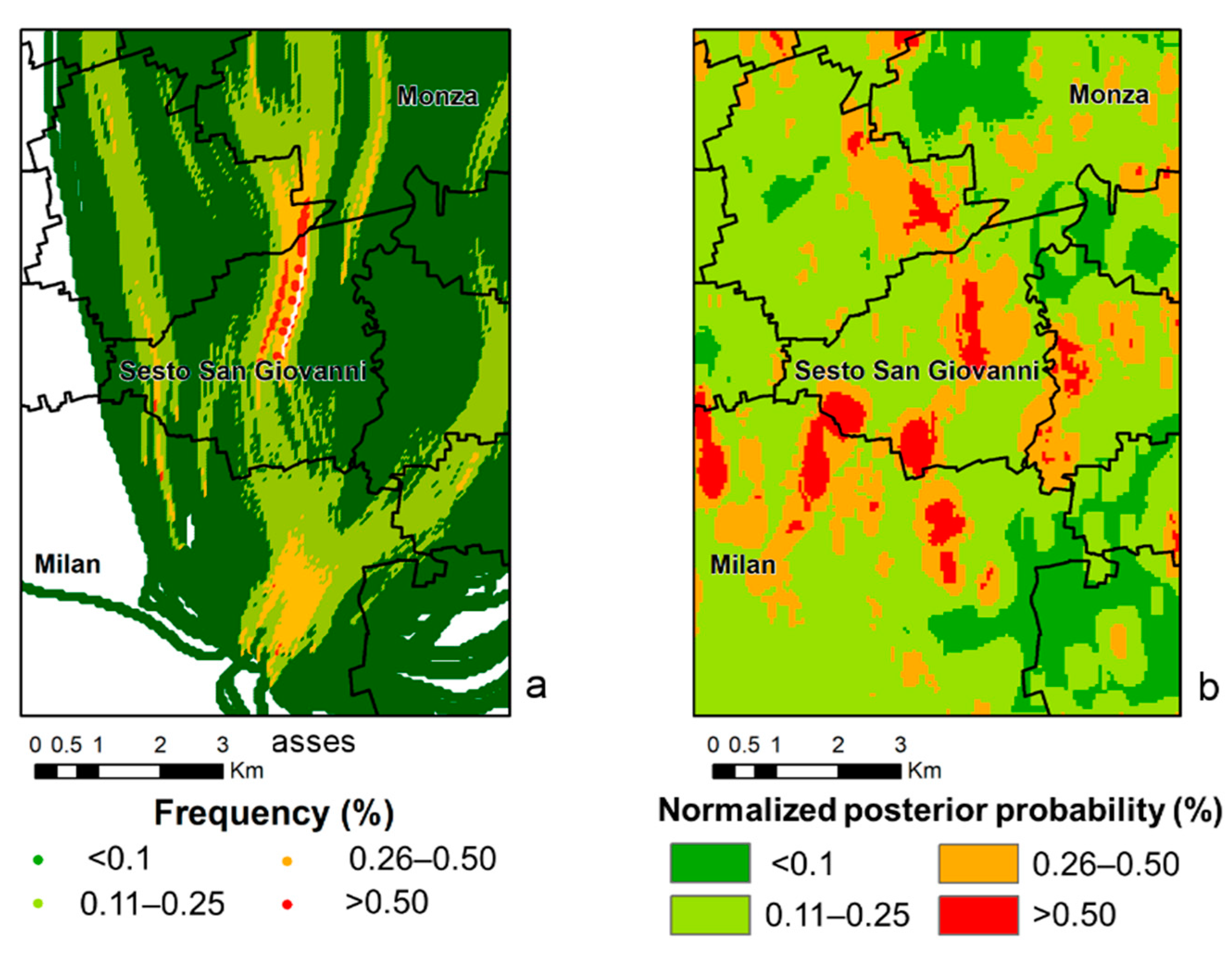
4.2. Predictive Responses and Susceptibility Map
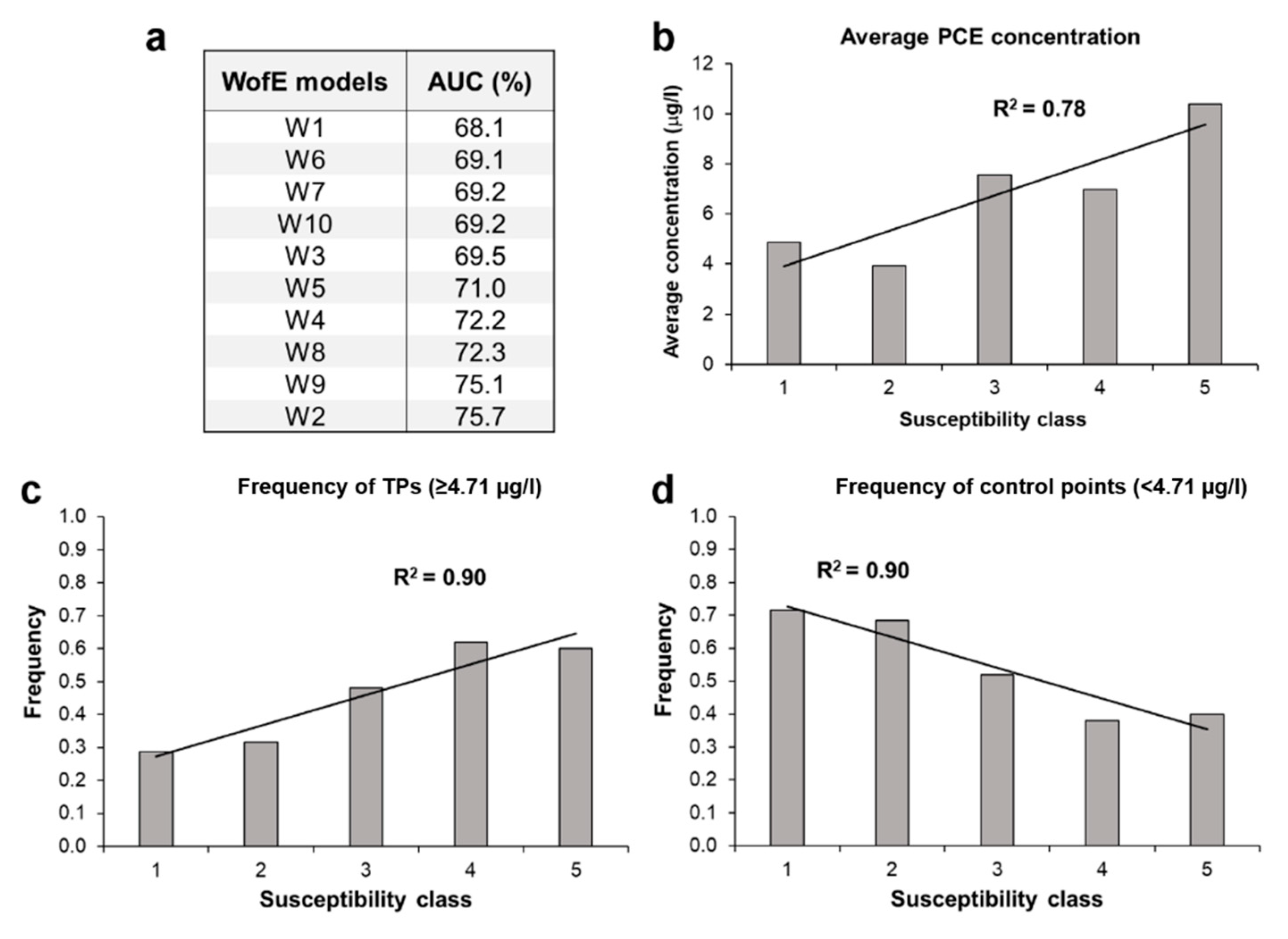
4.3. Reliability and Validation
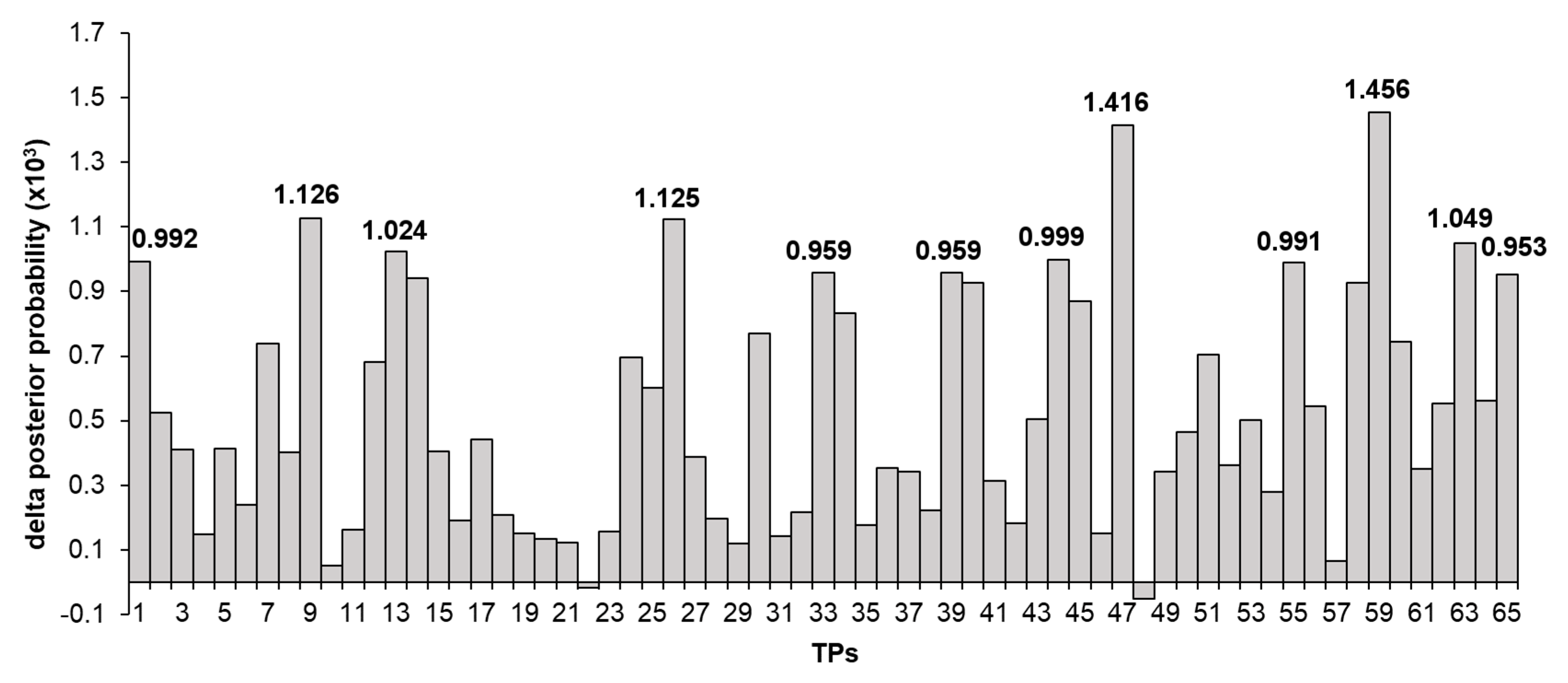
4.4. Evaluation of the Efficiency of the Monitoring Network
5. Discussion
Comparison between the Spatial Statistical Approach and the Numerical Stochastic Approach
6. Conclusions
- spatially evaluate the likelihood of having active MPS in a contaminated groundwater area;
- relate their impact on the shallow aquifer to the hydrogeological features of the area;
- highlight the presence of diffuse contamination due to both “historical” (that is, already removed) and recent MPS;
- test the efficiency of the monitoring network in properly characterizing the contamination in the aquifer, both for reducing the uncertainty in identifying the contaminated area and for eliminating unnecessary monitoring points.
Author Contributions
Funding
Acknowledgments
Conflicts of Interest
References
- European Community. Directive 2006/118/EC of the European Parliament and of the Council of 12 December 2006 on the Protection of Groundwater Against Pollution and Deterioration. Off. J. Eur. Union 2006, 19, 19–31. [Google Scholar]
- EEA—European Environment Agency. European Waters—Current Status and Future Challenges: Synthesis; Publications Office of the European Union: Luxembourg, 2012. [Google Scholar] [CrossRef]
- Lerner, D.N. Estimating Urban Loads of Nitrogen to Groundwater. Water Environ. J. 2003, 17, 239–244. [Google Scholar] [CrossRef]
- European Parliament. Directive (EU) 2016/2341 of the European Parliament and of the Council of 14 December 2016 on the Activities and Supervision of Institutions for Occupational Retirement Provision (IORPs). Off. J. Eur. Union 2016, 354/37, 37–85. [Google Scholar]
- Petersen-Perlman, J.D.; Megdal, S.B.; Gerlak, A.K.; Wireman, M.; Zuniga-Teran, A.A.; Varady, R.G. Critical Issues Affecting Groundwater Quality Governance and Management in the United States. Water 2018, 10, 735. [Google Scholar] [CrossRef]
- Kuroda, K.; Fukushi, T. Groundwater Contamination in Urban Areas. In Groundwater Management in Asian Cities: Technology and Policy for Sustainability; Takizawa, S., Ed.; cSUR-UT Series: Library for Sustainable Urban Regeneration; Springer: Tokyo, Japan, 2008; pp. 125–149. ISBN 978-4-431-78399-2. [Google Scholar] [CrossRef]
- Masetti, M.; Poli, S.; Sterlacchini, S. The Use of the Weights-of-Evidence Modeling Technique to Estimate the Vulnerability of Groundwater to Nitrate Contamination. Nat. Resour. Res. 2007, 16, 109–119. [Google Scholar] [CrossRef]
- Nolan, B.T.; Hitt, K.J.; Ruddy, B.C. Probability of Nitrate Contamination of Recently Recharged Groundwaters in the Conterminous United States. Environ. Sci. Technol. 2002, 36, 2138–2145. [Google Scholar] [CrossRef] [PubMed]
- Regione Lombardia. Deliberazione Della Giunta Regionale n. IX/3510 del 23/05/2012. Realizzazione Degli Interventi di Bonifica ai sensi dell’art. 250 del D.Lgs. 152 del 3 Aprile 2006. Programmazione Economico-Finanziaria 2012/2014. Available online: www.regione.lombardia.it/amministrazione_aperta/45740358 (accessed on 5 June 2019).
- Somaratne, N.; Zulfic, H.; Ashman, G.; Vial, H.; Swaffer, B.; Frizenschaf, J. Groundwater Risk Assessment Model (GRAM): Groundwater Risk Assessment Model for Wellfield Protection. Water 2013, 5, 1419–1439. [Google Scholar] [CrossRef]
- Alberti, L.; Colombo, L.; Formentin, G. Null-space Monte Carlo particle tracking to assess groundwater PCE (Tetrachloroethene) diffuse pollution in north-eastern Milan functional urban area. Sci. Total Environ. 2018, 621, 326–339. [Google Scholar] [CrossRef]
- Provincia di Milano. Indagini Sulla Presenza di Composti Organo-Alogenati Nelle Acque di Falda della Provincia di Milano; S.I.F. Provincia di Milano: Milano, Italy, 1992.
- Alberti, L.; Cantone, M.; Colombo, L.; Lombi, S.; Piana, A. Numerical modeling of regional groundwater flow in the Adda-Ticino Basin: Advances and new results. IJG 2016, 41/2016. [Google Scholar] [CrossRef]
- Bini, A. Stratigraphy, chronology and palaeogeography of Quaternary deposits of the area between the Ticino and Olona rivers (Italy-Switzerland). Geol. Insubrica 1997, 2, 21–46. [Google Scholar]
- Cavallin, A.; Francani, V.; Mazzarella, S. Studio idrogeologico della pianura compresa fra Adda e Ticino. Costruzioni 1983, 326/327, 39. [Google Scholar]
- Regione Lombardia; ENI Divisione AGIP. Geologia Degli Acquiferi Padani Della Regione Lombardia [Geology of the Po Valley Aquifers in Lombardy Regio.]; S.EL.CA.: Firenze, Italy, 2001.
- ARPA Lombardia. PROGETTO PLUMES. Available online: http://www.regione.lombardia.it/wps/portal/istituzionale/HP/DettaglioRedazionale/istituzione/direzioni-generali/direzione-generale-ambiente-e-clima/piano-per-inquinamento-diffuso (accessed on 5 June 2019).
- Francani, V.; Beretta, G.P.; Avanzini, M.; Nespoli, M. Indagine Preliminare Sull’uso Sostenibile Delle Falde Profonde in Provincia di Milano [Preliminary Survey About Sustainable use of Deeper Groundwater in the Milan Province]; Ed. C.A.P.: Milano, Italy, 1995. [Google Scholar]
- Afifi, A.; May, S.; Clark, V.A. Computer-Aided Multivariate Analysis, 4th ed.; Chapman and Hall/CRC: Boca Raton, FL, USA, 2003. [Google Scholar]
- Everitt, B.S.; Landau, S.; Leese, M.; Stahl, D. Cluster Analysis, 5th ed.; John Wiley & Sons, Ltd.: Hoboken, NJ, USA, 2011; ISBN 978-0-470-97781-1. [Google Scholar] [CrossRef]
- Vega, M.; Pardo, R.; Barrado, E.; Debán, L. Assessment of seasonal and polluting effects on the quality of river water by exploratory data analysis. Water Res. 1998, 32, 3581–3592. [Google Scholar] [CrossRef]
- Alberti, L.; Azzellino, A.; Colombo, L.; Lombi, S. Use of cluster analysis to identify tetrachloroethylene pollution hotspots for the transport numerical model implementation in urban functional area of Milan, Italy. In Proceedings of the SGEM2016 Conference Proceedings, Albena, Bulgaria, 30 June–6 July 2016; Volume 1, pp. 723–730. [Google Scholar] [CrossRef]
- ARPA Lombardia. PROGETTO PLUMES - Integrazione. Available online: http://www.regione.lombardia.it/wps/portal/istituzionale/HP/DettaglioRedazionale/istituzione/direzioni-generali/direzione-generale-ambiente-e-clima/piano-per-inquinamento-diffuso (accessed on 5 June 2019).
- Colombo, L. Statistical methods and transport modeling to assess PCE hotspots and diffuse pollution in groundwater (Milan FUA). Acque Sotter. Ital. J. Groundw. 2017, 6, 15–24. [Google Scholar] [CrossRef]
- Azzellino, A.; Colombo, L.; Lombi, S.; Marchesi, V.; Piana, A.; Andrea, M.; Alberti, L. Groundwater diffuse pollution in functional urban areas: The need to define anthropogenic diffuse pollution background levels. Sci. Total Environ. 2019, 656, 1207–1222. [Google Scholar] [CrossRef]
- Bonham-Carter, G.F. Geographic Information Systems for Geoscientists: Modelling with GIS; Pergamon Press: New York, NY, USA, 1994. [Google Scholar]
- Raines, G.L.; Bonham-Carter, G.F.; Kamp, L. Predictive probabilistic modeling using ArcView GIS. ArcUser 2000, 3, 45–48. [Google Scholar]
- Agterberg, F.P.; Bonham-Carter, G.F.; Cheng, Q.; Wright, D.F. Weights of evidence modeling and weighted logistic regression for mineral potential. In Computers in Geology-25 Years of Progress; Davis, J.C., Herzfeld, U.C., Eds.; Oxford University Press: New York, NY, USA, 1993; pp. 13–23. [Google Scholar]
- Raines, G.L. Evaluation of Weights of Evidence to Predict Epithermal-Gold Deposits in the Great Basin of the Western United States. Nat. Resour. Res. 1999, 8, 257–276. [Google Scholar] [CrossRef]
- Poli, S.; Sterlacchini, S. Landslide Representation Strategies in Susceptibility Studies using Weights-of-Evidence Modeling Technique. Nat. Resour. Res. 2007, 16, 121–134. [Google Scholar] [CrossRef]
- Goetz, J.N.; Brenning, A.; Petschko, H.; Leopold, P. Evaluating machine learning and statistical prediction techniques for landslide susceptibility modeling. Comput. Geosci. 2015, 81, 1–11. [Google Scholar] [CrossRef]
- Lee, S.; Kim, Y.-S.; Oh, H.-J. Application of a weights-of-evidence method and GIS to regional groundwater productivity potential mapping. J. Environ. Manag. 2012, 96, 91–105. [Google Scholar] [CrossRef]
- Madani, A.; Niyazi, B. Groundwater potential mapping using remote sensing techniques and weights of evidence GIS model: A case study from Wadi Yalamlam basin, Makkah Province, Western Saudi Arabia. Environ. Earth Sci 2015, 74, 5129–5142. [Google Scholar] [CrossRef]
- Arthur, J.D.; Wood, H.A.R.; Baker, A.E.; Cichon, J.R.; Raines, G.L. Development and Implementation of a Bayesian-based Aquifer Vulnerability Assessment in Florida. Nat. Resour. Res. 2007, 16, 93–107. [Google Scholar] [CrossRef]
- Uhan, J.; Vižintin, G.; Pezdič, J. Groundwater nitrate vulnerability assessment in alluvial aquifer using process-based models and weights-of-evidence method: Lower Savinja Valley case study (Slovenia). Environ. Earth Sci. 2011, 64, 97–105. [Google Scholar] [CrossRef]
- Stevenazzi, S.; Masetti, M.; Beretta, G.P. Groundwater vulnerability assessment: From overlay methods to statistical methods in the Lombardy Plain area. Acque Sotter. Ital. J. Groundw. 2017, 6, 17–27. [Google Scholar] [CrossRef]
- Caniani, D.; Lioi, D.S.; Mancini, I.M.; Masi, S. Hierarchical Classification of Groundwater Pollution Risk of Contaminated Sites Using Fuzzy Logic: A Case Study in the Basilicata Region (Italy). Water 2015, 7, 2013–2036. [Google Scholar] [CrossRef]
- Sawatzky, D.L.; Raines, G.L.; Bonham-Carter, G.F.; Looney, C.G. Spatial Data Modeller (SDM): ArcMAP 9.3 Geoprocessing Tools for Spatial Data Modelling Using Weights of Evidence, Logistic Regression, Fuzzy Logic and Neural Networks. 2009. Available online: http://www.ige.unicamp.br/sdm/ (accessed on 5 June 2019).
- Masetti, M.; Sterlacchini, S.; Ballabio, C.; Sorichetta, A.; Poli, S. Influence of threshold value in the use of statistical methods for groundwater vulnerability assessment. Sci. Total Environ. 2009, 407, 3836–3846. [Google Scholar] [CrossRef] [PubMed]
- Sorichetta, A.; Masetti, M.; Ballabio, C.; Sterlacchini, S. Aquifer nitrate vulnerability assessment using positive and negative weights of evidence methods, Milan, Italy. Comput. Geosci. 2012, 48, 199–210. [Google Scholar] [CrossRef]
- Chung, C.-J.F.; Fabbri, A.G. Probabilistic Prediction Models for Landslide Hazard Mapping. Photogramm. Eng. Remote Sens. 1999, 65, 1389–1399. [Google Scholar]
- Sorichetta, A.; Masetti, M.; Ballabio, C.; Sterlacchini, S.; Beretta, G.P. Reliability of groundwater vulnerability maps obtained through statistical methods. J. Environ. Manag. 2011, 92, 1215–1224. [Google Scholar] [CrossRef]
- Stevenazzi, S.; Masetti, M.; Nghiem, S.V.; Sorichetta, A. Groundwater vulnerability maps derived from a time-dependent method using satellite scatterometer data. Hydrogeol. J. 2015, 23, 631–647. [Google Scholar] [CrossRef]
- Goovaerts, P. Geostatistics for Natural Resources Evaluation (Applied Geostatistics); Oxford Univ. Press: New York, NY, USA, 1997. [Google Scholar]
- Anderson, M.P.; Woessner, W.W. Applied Groundwater Modeling: Simulation to Flow and Advective Transport, 1st ed.; Academic Press: San Diego, CA, USA, 1992. [Google Scholar]
- DUSAF-Destinazione d’Uso dei Suoli Agricoli e Forestali [Land use database]. ERSAF—Ente Regionale per i Servizi all’Agricoltura e alle Foreste. Available online: http://www.cartografia.regione.lombardia.it/ (accessed on 1 April 2019).
- Tonkin, M.; Doherty, J. Calibration-constrained Monte Carlo analysis of highly parameterized models using subspace techniques. Water Resour. Res. 2009, 45. [Google Scholar] [CrossRef]


| Susceptibility Classes | 1 | 2 | 3 | 4 | 5 | Sum 1 | |
|---|---|---|---|---|---|---|---|
| Coefficient of Variation Categories | |||||||
| 0–25% | 0.1 | 0.1 | 0.9 | 0.2 | 0.0 | 1.3 | |
| 25–50% | 13.1 | 10.6 | 12.4 | 10.8 | 1.5 | 48.5 | |
| 50–75% | 3.5 | 1.2 | 7.0 | 11.8 | 3.1 | 26.7 | |
| 75–100% | 1.7 | 2.3 | 4.2 | 3.4 | 1.2 | 12.8 | |
| ≥100% | 4.0 | 1.9 | 2.8 | 1.6 | 0.3 | 10.6 | |
| Sum 2 | 22.4 | 16.1 | 27.4 | 27.9 | 6.2 | 100 | |
© 2019 by the authors. Licensee MDPI, Basel, Switzerland. This article is an open access article distributed under the terms and conditions of the Creative Commons Attribution (CC BY) license (http://creativecommons.org/licenses/by/4.0/).
Share and Cite
Pollicino, L.C.; Masetti, M.; Stevenazzi, S.; Colombo, L.; Alberti, L. Spatial Statistical Assessment of Groundwater PCE (Tetrachloroethylene) Diffuse Contamination in Urban Areas. Water 2019, 11, 1211. https://doi.org/10.3390/w11061211
Pollicino LC, Masetti M, Stevenazzi S, Colombo L, Alberti L. Spatial Statistical Assessment of Groundwater PCE (Tetrachloroethylene) Diffuse Contamination in Urban Areas. Water. 2019; 11(6):1211. https://doi.org/10.3390/w11061211
Chicago/Turabian StylePollicino, Licia C., Marco Masetti, Stefania Stevenazzi, Loris Colombo, and Luca Alberti. 2019. "Spatial Statistical Assessment of Groundwater PCE (Tetrachloroethylene) Diffuse Contamination in Urban Areas" Water 11, no. 6: 1211. https://doi.org/10.3390/w11061211
APA StylePollicino, L. C., Masetti, M., Stevenazzi, S., Colombo, L., & Alberti, L. (2019). Spatial Statistical Assessment of Groundwater PCE (Tetrachloroethylene) Diffuse Contamination in Urban Areas. Water, 11(6), 1211. https://doi.org/10.3390/w11061211