Toward a Priori Evaluation of Relative Worth of Head and Conductivity Data as Functions of Data Densities in Inverse Groundwater Modeling

Abstract

Groundwater hydraulic head (H) measurements and point-estimates of hydraulic conductivity (K) both contain information about the K field. There is no simple, a priori estimate of the relative worth of H and K data. Thus, there is a gap in our conceptual understanding of the value of the K inversion procedure. Here, using synthetic calibration experiments, we quantified the worth of H and K data in terms of reducing calibrated K errors. We found that normalized K error $e_K$ could be approximated by a polynomial function with first-order terms of H and K data densities ${\mu }_H$ and ${\mu }_K$, which have been normalized by the correlation lengths of the K field, and a mutually inhibitive interaction term. This equation can be applied to obtain a rough estimate of the uncertainty prior to the inversion for a case with a similar configuration. The formulation suggests that the inversion is valuable even without K data. The relative worths of H and K depend heavily on existing data densities and heterogeneity. K can be ten times more informative when it is sparse. Noise perturbation experiments show that we should incorporate noisy K data when K is sparse, but not a large amount of low-quality K estimates. Our conclusions establish a crude, baseline estimate of the value of calibration. A similar assessment method for information content can be employed for more complex problems.

1. Introduction

The hydraulic conductivity (K) is a porous media property that is of great importance to various applications including integrated hydrologic modeling [1,2], contaminant fate and transport predictions, evaluation of groundwater resources [3], and analytical modeling [4]. On the one hand, K can be inferred from pumping tests [5] or lithological estimates. Typically, K values are not independently distributed but auto-correlated in space [6]. Therefore, one K measurement provides some information not only about the site, but also about the adjacent region. On the other hand, K can also be estimated inversely by calibrating a suitable groundwater flow model to an observed hydraulic head (H) using a prescribed recharge. There are mature inversion packages such as model-independent parameter estimation and uncertainty analysis (PEST) [7], which adjust K values, so that simulated H is close to observed data. Often, they make use of available (but sparse) known K data points and geostatistical models to constrain (or, in machine learning terminology, regularize) the inversion process. Therefore, both H and scattered K data help reduce the uncertainty, i.e., they both carry information content about the K field.

Despite a significant body of literature on the information content (or data worth) of K measurements, which we will summarize below, a conceptual knowledge gap exists regarding the relative value of H data and the K inversion process. Recently, integrated hydrologic modeling studies, e.g., [8,9,10,11], have relied on large-scale estimates of hydraulic conductivity, e.g., [12], for parameterizing K, but these estimates may not offer adequate resolution and accuracy for local groundwater modeling purposes. Integrated modeling studies often skip the step of K inversion. A part of the reason may be that, prior to conducting the calibration, there is no method to estimate how much uncertainty can be reduced by this process. On the other hand, it is common to find studies where the calibrated K fields are presented without associated uncertainty estimates. Given the amount of available data, how much uncertainty in the K field can be reduced by calibrating K to H? What is the value of adding point-scale K measurements, which are inherently noisy, for improving the accuracy of calibration? What is the value of securing more K or H measurements? A-priori answers to these questions may help gauge the expected return of the calibration effort prior to carrying out the work.

Sifting through literature, we found that there are no simple answers to these inquiries. Previous studies on optimal experimental designs have provided valuable contributions to understanding the data worth of K measurements [13,14,15]. Their objectives were mostly to design the optimal way of obtaining new K data points for different purposes. For instance, James et al. [13] used a Bayesian data-worth framework to determine the location of data points that maximize their value in reducing the total remediation cost, where the pollutant plume was uncertain with regard to both location and extent. Neuman et al. [15] extended data-worth analysis by using the Bayesian model averaging approach to maximize the cost-benefit of K data points. Freeze et al. [16] also optimized the locations of measurements to minimize uncertainties with aquitard continuity and K distribution, while considering minimized economic regret. Tucciarelli et al. [17] employed a chance-constrained stochastic technique to find the best number and locations of additional measurements, which could result in a minimum total cost of data acquisition and groundwater reclamation. One similar chance-constrained model was coupled to an integer-programing sampling network design model in Wagner [14] in order to optimize pumping and sampling strategies. The worth of data can also be evaluated via sequential data assimilation methods such as ensemble Kalman filtering [18,19].

Despite the large body of literature, to the best of our knowledge, no work compared the value of H data in the calibration of K. In other words, the information content of H data was not given sufficient attention. However, the comparison between H and K values can be both challenging and nuanced due to the many strategies that were utilized to optimize spatial locations of data points, each with different objectives, constraints, and results. Therefore, we turn to a more modest question, “With a fixed, regularly spaced configuration of data locations, what is the value of H and K data, respectively?”

Centered around the abovementioned main question, this paper is organized to answer the following three sub-questions: (1) In a uniformly distributed data setting, can we describe calibrated K and H errors as functions of (preferably dimensionless) data densities, and are errors functions of recharge and boundary conditions? (2) How do the worths of K and H compare under different scenarios of H and K densities? (3) How do uncertainties with known K values impact our analyses? In the interest of reducing the dimensionality of the problem, we seek to non-dimensionalize data densities and errors with respect to the spatial heterogeneity of K. We will verify that the resulting numbers are truly non-dimensional characterizations of system features. Dimensionless numbers have been used in hydrological analysis with success. For example, see Haitjema and Mitchell-Bruker [20] for the water table ratio and Li et al. [21] for the six dimensionless numbers characterizing watershed hydrologic response types. These dimensional numbers, when verified, reveal underlying hydrologic dynamics and allow the conclusion to be migrated to different scales.

The advantage of the simple configuration is that the cause (data density and other factors) and effects (calibrated K error) can be clearly ascertained. While we acknowledge that such a configuration is rare, and the real-world is much more complex, our effort at least provides a baseline scenario that sheds insights and allows comparison with other strategies. As a result, it is a step forward in improving our understanding. Although they play important roles in groundwater modeling, the storage coefficient and transient modeling are outside of the scope of the present study. Furthermore, even though groundwater can be studied using Richards equation [22,23,24,25,26] as an integrated component of the hydrologic system [27], or the Boussinesq approximation [28], we focus on the saturated groundwater flow.

2. Methodology

2.1. Experimental Design

As discussed above, we used uniformly distributed H observations to make the study tractable. A prescribed fraction of the H data points were randomly sampled and assumed to have K estimates. Several realizations of such selections were prepared and tested in the calibrations. The collocation of H and K data points occurs because when a fine-scale K estimate is recorded, e.g., from pumping test, a water level reading can normally be obtained. We assumed a steady-state, 2D unconfined aquifer with uniform recharge.

The worth of data, in the context of this paper, is defined as the reduction of calibrated H and K error due to the inclusion of more data. As inverse modeling error is relative to the range of K variability, its absolute value has limited meaning, and is also not transferrable. Hence, we defined a dimensionless calibrated K error, $e_K$, as the normalized root-mean-squared logarithmic error (RMSLE) between log-transformed calibrated and synthetic K:

$$\begin{gathered} RMSLE=\sqrt{\frac{{{\displaystyle \sum }}_{i=1}^N{\left[\log \left(K_i^o\right)-\log \left(K_i^c\right)\right]}^2}{N}} \\ {e}_K=\frac{RMSLE}{\log (P_{90})-\log \left(P_{10}\right)} \end{gathered}$$

(1)

where $K_i^o$ and $K_i^c$ are the synthetic and calibrated hydraulic conductivity values at the i-th location in the domain, respectively. N is the total number of cells in the domain, and $\log (P_{90})$ and $\log \left(P_{10}\right)$ are the 90th and 10th percentiles of synthetic conductivity values, with their differences characterizing the variability. Using these values instead of maximum and minimum values avoids skewing the error estimate by extreme values in the stochastically generated K fields. Other percentiles may also be considered. We will show that the normalization removes the dependence of error on the variability of the K field.

Similarly, the normalized error of H, $e_H$, was calculated for the collection of synthetic wells, as a normalized root mean squared error (RMSE).

$$\begin{gathered} RMSE=\sqrt{\frac{{{\displaystyle \sum }}_{i=1}^n{\left(H_i^o-H_i^c\right)}^2}{n}} \\ {e}_H=\frac{RMSE}{H_{max}-H_{min}} \end{gathered}$$

(2)

where $H_i^o$ and $H_i^c$ are the “observed” and simulated groundwater head at the i-th synthetic H observation locations, respectively, and $H_{max}$ and $H_{min}$ are the maximum and minimum groundwater head across the domain corresponding to the synthetic K field.

2.1.1. Synthetic Domain

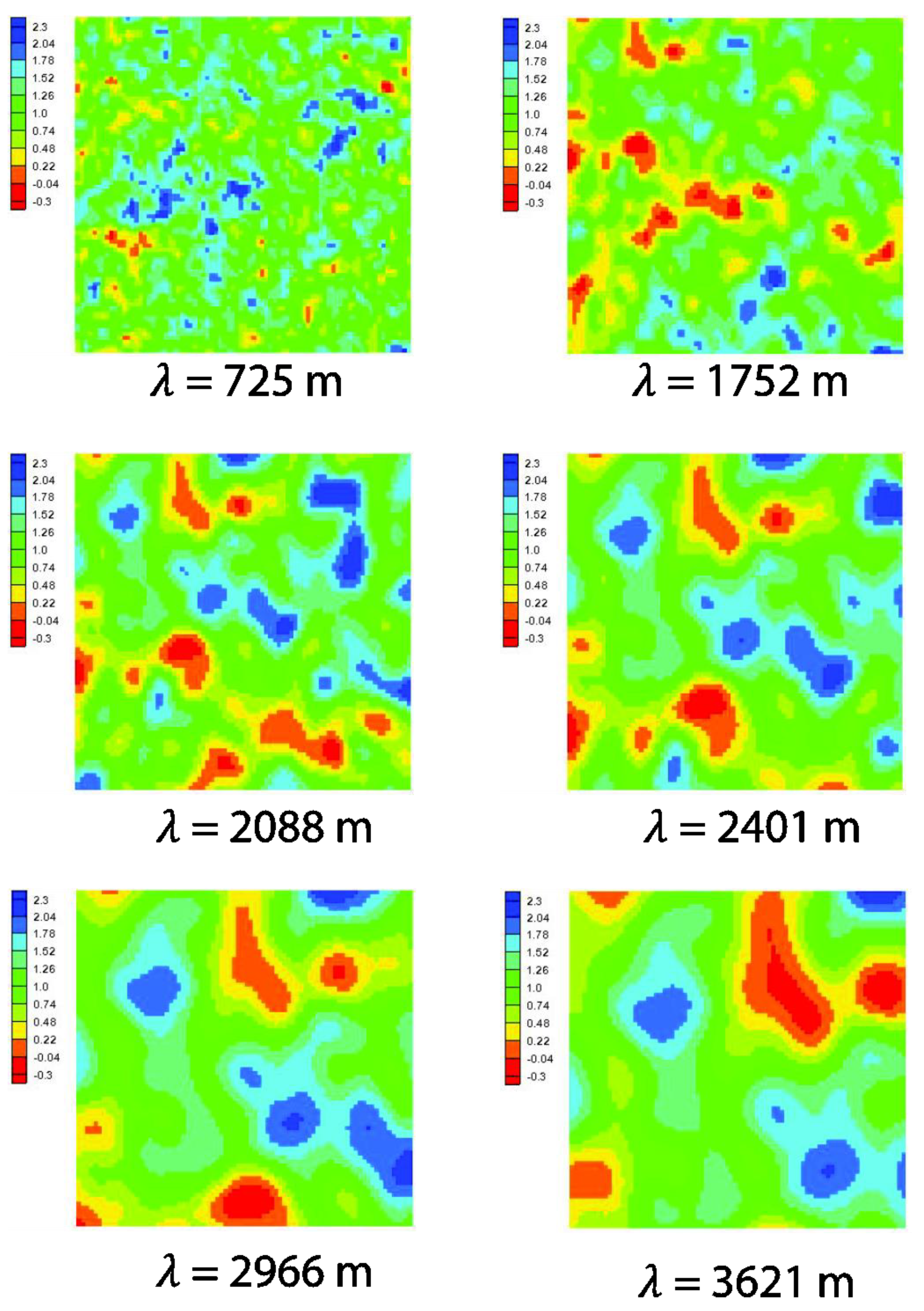
Our computational domain is a rectangular unconfined aquifer. Six random K fields (Figure 1) distinguished by different spatial correlation lengths, $\lambda$, were generated with FIELDGEN, a supplemental utility for the model water flow and balance simulation model (WaSiM) [29]. We manually varied the mean, standard deviation, and correlation length when running FIELDGEN to generate the fields with different $\lambda$. The number of fields was chosen as a balance of the total work load and the representation of heterogeneity. The range of $\lambda$ that we tested ensured that, at the largest $\lambda$, there are at least several clusters of high and low K values. Further increasing the range of $\lambda$ will make it too labor intensive and computationally expensive to complete our numerical experiments. The K fields are all of log-normal distribution, with K values between 0.5 m day⁻¹ to 200 m day⁻¹. It needs to be noted that the absolute value of this range is irrelevant if non-dimensionalization of the system is valid, which means the conclusions are only dependent on the dimensionless numbers. Then, we fitted a spherical model to the extracted empirical semi-variogram. The formula for the spherical model is:

$$\gamma \left(h\right)=\{\begin{array}{ll}c\left[1.5\frac{h}{\lambda }-0.5{\left(\frac{h}{\lambda }\right)}^3\right],& if h\le \lambda \\ c,& if h>\lambda \end{array}$$

(3)

where $\gamma \left(h\right)$ is the empirical semi-variogram calculated from the generated field, h is the lag distance, c is the sill, and $\lambda$ is the correlation length. We used a bound-constrained version of the “fminsearch” command from Matlab^® [30] to find the c and $\lambda$ that minimized the sum of squared differences between the theoretical model in Equation (3) and the empirical variogram. We cut off the empirical semi-variogram at 8000 m before fitting the variogram model.

The model domain spans 8000 m in both horizontal coordinate directions. The top and bottom elevations were 150 m and −100 m, respectively. Except for the ones that test the effects of recharge (Section 2.4), all experiments employed a uniform recharge of 500 mm/year. Again, if the dimensionless analysis is found to be valid, what is important for the groundwater flow system is the ratio of recharge to conductivity. By default, the eastern side was assigned a specified head (Dirichlet) boundary condition, with a water head of 130 m, while the three other sides were set as no-flow boundaries. However, the eastern and western boundary conditions were varied to test the effects of different recharge and boundary conditions.

2.1.2. Synthetic Observations of H and K

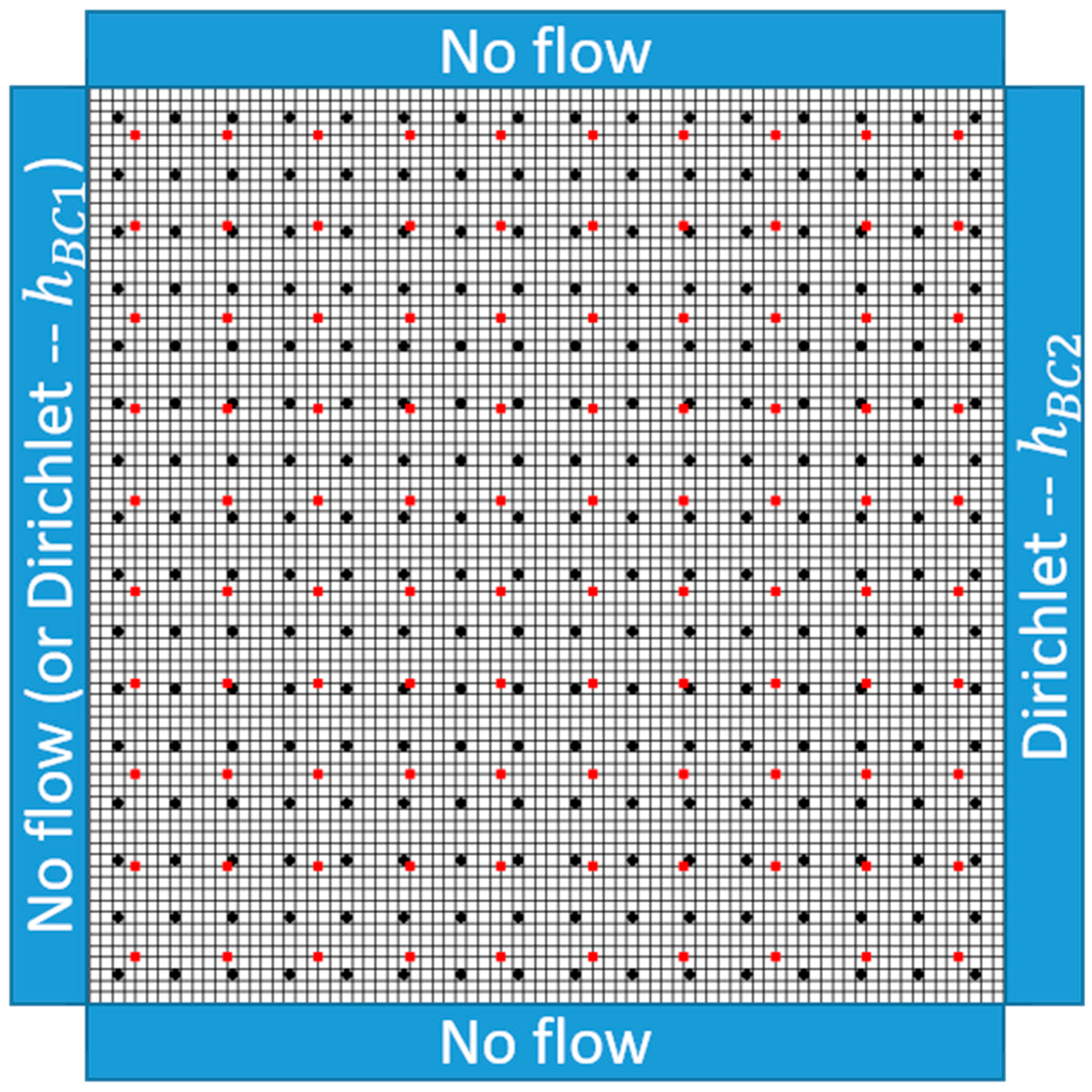
The calibration of a K field requires observed H values and optionally known K values [31,32]. The locations of synthetic H observations were evenly distributed throughout the domain, with an interval of 500 m leading to 256 virtual wells (Figure 2). While the data may look dense, if the correlation length is small, the data is relatively sparse. In terms of calibrated K error, as we will show later, the problem is dimensionless, in the sense that only the ratio between data density and correlation length matters. For a field with a small $\lambda$ as in Figure 1a, the data is not dense after all. The water head at each observation well was extracted from a forward simulation with the aforementioned synthetic K fields, recharge, and boundary conditions. We randomly assigned known K values to x% of the observation wells.

2.2. Inverse Modeling

We used MODFLOW-2000 [33] as the groundwater flow model, and the model-independent parameter estimation and uncertainty analysis (PEST) [34] as the inverse modeling tool. PEST estimates K with the assistance of pilot points, each of which carries an initial K value that is used in calibrations and interpolated to all the grid cells in the domain. We set pilot points at the centroid of each 600 × 600 square box of the domain (see Figure 2). The inversion procedure in PEST adjusts K with an iterative approach to minimize the following objective function:

$$\begin{gathered} {\Phi }_m={\left({\mathit{H}}^{\mathit{o}}-\mathit{M}\left(\mathit{K}\right)\right)}^T\mathit{Q}\left({\mathit{H}}^{\mathit{o}}-\mathit{M}\left(\mathit{K}\right)\right) \\ {\Phi }_g= {\Phi }_m+\alpha {\Phi }_r \\ {\mathit{K}}^{\mathit{c}}=\underset{\mathit{K}}{\mathit{a}\mathit{r}\mathit{g}\mathit{m}\mathit{i}\mathit{n}}\left({\mathit{\Phi }}_{\mathit{g}}\right) \end{gathered}$$

(4)

where ${\Phi }_m$ is the unregularized objective function, ${\Phi }_r$ is a regularization term with $\alpha$ as a parameter, ${\Phi }_g$ is the global objective function, vector $\mathit{K}$ contains the conductivity values of the field, ${\mathit{H}}^{\mathit{o}}$ is the observation, and Q is a weight matrix used to define greater contributions of certain pairs of observations. In the present simulation, a uniform weight is assigned to all K observations. $\mathit{M}$ is the model that predicts the system responses, given the parameter set $\mathit{K}$, and ${\mathit{K}}^{\mathit{c}}$ is the calibrated K field that minimizes ${\mathit{\Phi }}_{\mathit{g}}$.

Without $\alpha {\Phi }_r$, the inversion process can be non-unique, which means that different sets of parameter values may produce similar outcomes. K could be overfitted, which may lead to large errors when used in the predictive mode [31,34]. To reduce overfitting, $\alpha {\Phi }_r$ implements a penalization procedure called Tikhonov Regularization [35], which introduces geospatial structure as a constraint in the calibration. ‘Regularization’ here is synonymous to ‘penalization.’ The regularization term is:

$${\Phi }_r={\left(\mathit{d}-\mathit{R}\left(\mathit{K}\right)\right)}^T{\mathit{Q}}_{\mathit{r}}\left(\mathit{d}-\mathit{R}\left(\mathit{K}\right)\right)$$

(5)

where Q_r is a diagonal matrix consisting of squared weights assigned to each observation, R is a regularization operator that expresses a certain geostatistical constraint, e.g., the difference between a trial parameter value and the parameter value at a site, given neighbors’ values (and a variogram model), and $\mathit{d}$ is a ‘system-preferred’ state, which is 0 in this case.

In PEST, $\alpha$ is estimated together with calibration. With the help of a definition for an ‘acceptably good’ ${\Phi }_m$ value, ${\Phi }_m^1$, PEST found the $\alpha$ that minimizes ${\Phi }_r$ while satisfying that ${\Phi }_m$ is no greater than ${\Phi }_m^1$. This regularization penalizes parameter values that are far from the value expected of geostatistical models (built from data). The system can estimate more pilot points than there are observations, because each new pilot points is automatically accompanied by a spatially interpolated value. The algorithm attempts to ensure that the extra degrees of freedom, which carry little information, are discarded [36]. The interpolation method we selected was Kriging with a spherical model. The number of pilot points was set to 40% of H data points across all experiments. Considering the objective of the study, we did not test the fraction of pilot points as a control variable.

2.3. Non-Dimensionalization of Data Density and Errors

If we draw our conclusions as a function of dimensionless numbers, they are more broadly applicable than dimensional ones. The density of observation data needs to be examined relative to the spatial heterogeneity of the field, which is characterized by $\lambda$. Smaller $\lambda$ indicates a more rapid varying K in space, which requires more observational data to constrain. To reduce the degrees of freedom, we propose a dimensionless number, the effective data density, ${\mathsf{\mu }}_H$, which quantifies the ratio between the correlation length and square root of data density:

$${\mathsf{\mu }}_H=\frac{\lambda }{d_H}=\frac{\lambda }{\sqrt{A/n}}$$

(6)

where A is the domain area, n is the number of wells where H is measured, and $d_H$ measures the average distance between data points. ${\mathsf{\mu }}_H$ can be interpreted as “the square root of the number of H data points in a square box with an area of ${\mathsf{\lambda }}^2$”. A greater ${\mathsf{\mu }}_H$ indicates a slower variation of K relative to the distance between measurement points, and thus, more information about the H field.

Similarly, we can quantify the relative density of wells with known conductivity values, which are implemented by randomly assigning synthetic K values to x% of observation wells. It gives rise to the average distance between known K values, $d_K$:

$$d_K=\frac{d_H}{\sqrt{x\%}}$$

(7)

where x is the fraction of H observation wells with known K values. Then, similar to Equation (6), the dimensionless factor to quantify conductivity data acquisition ${\mathsf{\mu }}_K$ is derived as:

$${\mathsf{\mu }}_K=\frac{\lambda }{\sqrt{A/\left(n\times x\%\right)}}$$

(8)

The use of ${\mathsf{\mu }}_H$ and ${\mathsf{\mu }}_K$ allows us to greatly reduce the number of experiments and simplify the experimental design. If they can effectively and adequately characterize the system, we can avoid simultaneously varying the number of data points and spatial heterogeneity. Instead, we can adjust only the latter. To verify the validity of the dimensionless numbers, we compared the errors of calibrated K from a series of experiments, which contained different combinations of $\lambda$, $n$, and $x\%$ and produced similar dimensionless numbers. Five different ${\mathsf{\mu }}_H$ values and five different ${\mathsf{\mu }}_K$ were tested while keeping other variables constant. For each x% value other than zero, three sets of random locations were chosen for known K, leading to three separate calibrations. The results were then averaged to obtain the final calibration errors.

2.4. Recharge and Boundary Conditions

We examined the impacts of recharge and boundary conditions (BC) on calibration errors. Six recharge levels ranging between 100 mm/year and 1000 mm/year and two values of ${\mathsf{\mu }}_H$ were tested. To prevent the recharge from raising the water table above the ground surface, the Dirichlet boundary was set to 115 m. Other model settings were identical to the default.

We also tested the impacts of the Dirichlet boundary conditions. For this test and this test only, we applied another Dirichlet boundary to the western domain boundary (Figure 2 right panel). We ran model calibrations with six ${\mathsf{\mu }}_H$ values, while fixing ${\mathsf{\mu }}_K$ at zero. We also ran five ${\mathsf{\mu }}_K$ values while keeping ${\mathsf{\mu }}_H$ at 4.18. We compared calibrated H and K errors from these different recharges and BCs.

2.5. Experimental Design and Multivariate Polynomial Curve Fitting

We tested a total of 31 pairs of (${\mathsf{\mu }}_H, {\mathsf{\mu }}_K$). For each pair, where ${\mathsf{\mu }}_K$ is non-zero, we ran three random realizations of K fields. This experimental design resulted in a total of 79 calibration experiments. All experiments had the same domain geometries and locations of water head observations. Different ${\mathsf{\mu }}_H$ was achieved by employing K fields with different $\lambda$ (Figure 1), while keeping n constant.

We fitted error as a polynomial function (maximum second order) of ${\mathsf{\mu }}_H$ and ${\mathsf{\mu }}_K$ values:

$$e\left({\mathsf{\mu }}_H,{\mathsf{\mu }}_K\right)=\mathbf{P}\times \stackrel{\rightharpoonup }{\mathsf{\mu }}$$

(9)

where P is a vector of coefficients in polynomial fitting, $\stackrel{\rightharpoonup }{\mathsf{\mu }}=\left(1, {\mathsf{\mu }}_H, {\mathsf{\mu }}_H^2 ,\dots ,{\mathsf{\mu }}_K, {\mathsf{\mu }}_K^2 ,{\mathsf{\mu }}_H{\mathsf{\mu }}_K\right)$ is the vector of predictors, and $e\left({\mathsf{\mu }}_H,{\mathsf{\mu }}_K\right)$ is the calibration error. Our experiments were constrained within the range of $\mathsf{\mu }$ values. P was fitted using Matlab^® curvefitting Toolbox. The term ${\mathsf{\mu }}_H{\mathsf{\mu }}_K$ in Equation (9) represents an interaction term. A probability value (p-value) was calculated for the null hypothesis that the coefficient is equation to zero based on t-tests for each of the curve fitting coefficients. Furthermore, the goodness of fit was evaluated using the coefficient of determination (R²) and the root mean of squared error between the calibrated K/H errors and the values predicted by the polynomial function.

2.6. The Influence of Measurement Noise

The known K values that are supplied to the inversion algorithm can be estimated from pumping tests, lithology, specific capacity, and drawdown data, or conductivity test of samples [5]. In practice, regardless of which method is used, there will be errors. To study the impacts of K measurement noise on the calibrated K, we conducted perturbation experiments, where we added a synthetic noise to the observations. Since the K field is assumed to be log-normally distributed, we perturbed K values as:

$$\log \left(K\right)=\log \left(K^{*}\right)+\epsilon$$

(10)

where $K^{*}$ is the true conductivity value, K is what is supplied to the calibration algorithm, and $\epsilon ~N\left(0,{\sigma }_n\right)$ is a Gaussian noise with a standard deviation of ${\sigma }_n$. If ${\sigma }_n$ is 0.2, it means 33% of the data points are perturbed to be either 50% larger or 37% smaller than $K^{*}$. If ${\sigma }_n=1$, then 33% of the K data points are perturbed by more than an order of magnitude. The influence of the noise is quantified as an amplification factor:

$$\beta =\left(\frac{e_K^{}}{e_K^{*}}\right)$$

(11)

where $e_K^{*}=e_K^{}\left({\mathsf{\mu }}_H,{\mathsf{\mu }}_K,{\sigma }_n=0\right)$ is the average calibrated K error of the calibrations with noise-free K data, as defined in Equation (1), and $e_K$ is the error for calibrations with added noise. The experiment was very labor-intensive, as we tested M realizations of the noise and random selections of K positions. We could not regularly sample the three-dimensional parameter space of (${\mathsf{\mu }}_H,{\mathsf{\mu }}_K,{\sigma }_n$) space as we did earlier. Instead, we explored a few lines in that space. In addition, since the readings of groundwater head (or depth to the water table) are generally more accurate compared to the K noise, we ignored H errors to reduce the dimensionality of the analysis. For comparing the results to the cases without any K data, we also defined ${\beta }^0$:

$${\beta }^0=\frac{e_K^{}\left({\mathsf{\mu }}_H,{\mathsf{\mu }}_K=0,{\sigma }_n=0\right)}{e_K^{}\left({\mathsf{\mu }}_H,{\mathsf{\mu }}_K,{\sigma }_n=0\right)}$$

(12)

${\beta }^0$ is the ratio of errors between cases calibrated “without K data” and “with noise-free K data.” It can be compared with other $\beta$s because they have common denominators.

2.7. Relative Data Worth

We can calculate the reduction of K error with respect to one measurement point: $\frac{\mathsf{\Delta }{e}_K}{\mathsf{\Delta }{n}_H}$ and $\frac{\mathsf{\Delta }{e}_K}{\mathsf{\Delta }{n}_K}$. These values can be approximated numerically by calculating the increments in $e_K$ or $e_H$ (given by Equation (9)), as the number of data points increase. They can also be derived from the fitted polynomials in Equation (9). Then, we can examine two ratios that measure the relative worth of data:

$$\begin{gathered} R_{\mu }= \frac{\partial e_K}{\partial {\mu }_H}:\frac{\partial e_K}{\partial {\mu }_K} \\ {R}_n= \frac{\mathsf{\Delta }{e}_K}{\mathsf{\Delta }{n}_H}:\frac{\mathsf{\Delta }{e}_K}{\mathsf{\Delta }{n}_K} \end{gathered}$$

(13)

$R_{\mu }$ is the relative data worth ratio with respect to a unit increase in ${\mu }_H$ or ${\mu }_K$ and is only a function of these two factors. Since $\mu$ is a nonlinear function of $n$, far more data points are needed to increase a unit of $\mu$ when $\mu$ is high. This relationship can make $R_{\mu }$ difficult to interpret and use. $R_n$ indicates whether it is more beneficial to add an H or a K data point, which has a direct practical meaning. However, $R_n$ has three control variables: $n_H$, $n_K$ and $\mathsf{\lambda }$. We will show the influence of $n_H$, $n_K$ under two different $\mathsf{\lambda }$ values.

We considered the following two scenarios when calculating $R_n$: (A) A new K data point is always accompanied by a new H data point, which is relevant when we plan to install new wells. In this scenario, $\frac{\mathsf{\Delta }{\mu }_H}{\mathsf{\Delta }{n}_K}= \frac{\mathsf{\Delta }{\mu }_H}{\mathsf{\Delta }{n}_H} =\frac{\lambda }{2\sqrt{A{n}_H}}$; (B) we can add a K measurement without adding H data. This scenario is relevant when we can conduct a pumping test from an existing well, or extract K estimates from interpreting existing literature. Under this scenario, $\frac{\mathsf{\Delta }{\mu }_H}{\mathsf{\Delta }{n}_K}$ is 0. We denoted $R_n^{\prime } \mathrm{as}$ the data worth ratio calculated under scenario (B).

3. Results and Discussion

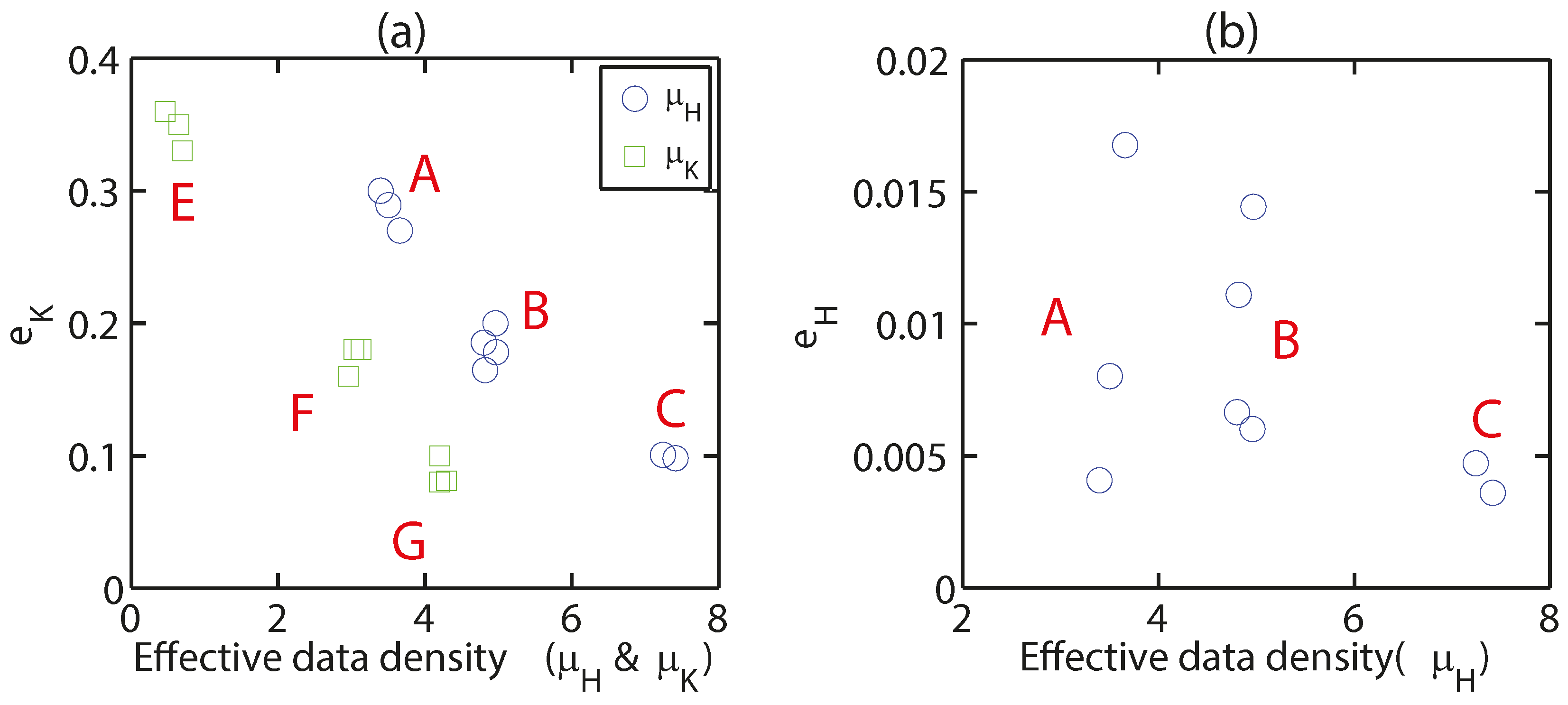
3.1. Verification of the Effectiveness of Non-Dimensionalization

Given similar ${\mathsf{\mu }}_H$ and ${\mathsf{\mu }}_K$ values, the normalized conductivity error $e_K$ is tightly clustered (Figure 3), although $\lambda$, $n$, and x% varied substantially (

Table A1. Experimental configurations and errors for the verifications of dimensionless numbers are shown in Figure 3.

Cluster	${\mathsf{\mu }}_{\mathit{H}}$	${\mathsf{\mu }}_{\mathit{K}}$	$\mathbf{\lambda }$	${\mathit{n}}_{\mathit{H}}$	${\mathit{n}}_{\mathit{K}}$	${\mathit{e}}_{\mathit{H}}$	${\mathit{e}}_{\mathit{K}}$
A	3.4	0	725	1444	0	0.0041	0.3
	3.5	0	1752	256	0	0.008	0.29
	3.66	0	2088	196	0	0.017	0.27
B	4.8	0	2088	361	0	0.006	0.19
	5	0	2401	256	0	0.007	0.2
	4.8	0	2966	169	0	0.011	0.17
	5	0	3621	121	0	0.014	0.08
C	7.2	0	3621	256	0	0.101	0.005
	7.4	0	2966	169	0	0.980	0.004
E	1.5	0.45	725	256	25	N/A	0.36
	1.4	0.64	725	256	49	N/A	0.35
	1.5	0.69	1751	49	16	N/A	0.33
F	3.1	2.95	1751	256	196	N/A	0.18
	3.4	3.13	2088	169	144	N/A	0.18
	4.3	3.04	2088	256	121	N/A	0.16
G	4.8	4.3	2401	256	196	N/A	0.081
	5.9	4.194	2966	256	121	N/A	0.08
	4.7	4.2	2088	324	256	N/A	0.1

). This behavior verified that ${\mathsf{\mu }}_H$ and ${\mathsf{\mu }}_K$ are effective dimensionless numbers to characterize $e_K$, which allowed us in only altering $\lambda$ in later experiments. In addition, Figure 3 suggested $e_K$ can be described as a smooth function of ${\mathsf{\mu }}_H$ and ${\mathsf{\mu }}_K$. In these preliminary experiments, we did not observe any non-monotonicity or fluctuations. Such smoothness and monotonicity serve as the basis of fitting a polynomial function to the relationships between normalized error and data densities.

However, we did not obtain a clustering pattern for water head error. The $e_H$ values showed obvious scattering even with similar ${\mathsf{\mu }}_H$ and ${\mathsf{\mu }}_K$. Therefore, it is meaningless to further test $e_H$. In summary, ${\mathsf{\mu }}_H$ and ${\mathsf{\mu }}_K$ are effective dimensionless numbers to characterize the system for $e_K$ but not for $e_H$. As a result, the conclusions to be drawn later for $e_K$ as a function of ${\mathsf{\mu }}_H$ and ${\mathsf{\mu }}_K$ were applicable to different $\lambda$, $x\%$, n combinations, while those for $e_H$ were only valid for ${\mathsf{\mu }}_H$ and ${\mathsf{\mu }}_K$ values that we specified.

3.2. Impact of Recharge and Boundary Condition on Model Calibration Errors

Normalized errors are independent of recharge (Figure 4a,b). Various recharge inputs lead to different water head ranges and, consequently, different absolute error values. However, after the error is normalized on the ranges of H and K, they become flat and non-responsive to recharge. In summary, these experiments show that the influence of recharge is linear, and can be removed by normalizing the error with respect to the range of values in the domain. Therefore, we no longer considered recharge in our factorial experiments.

Comparing $e_K~{\mu }_H$ and $e_K~{\mu }_K$ curves obtained with two different boundary conditions, we noted that the boundary condition had little impact and the two sets of curves almost overlapped (Figure 4c). The two boundary conditions tested were Dirichlet and Neumann, which approximate lakes, rivers (Dirichlet), impervious mountain blocks (Neumann), and so on. However, the same cannot be said about $e_H$: There are gaps between Dirichilet and Neumann BCs and the gaps are not constant (Figure 4d). The addition of Dirichlet boundary increases the water head error $e_H$ and makes calibration results more stochastic. These patterns mean that the conclusions to be drawn later in this paper with regard to $e_K$, but not $e_H$, can be generalized for many different situations, with little impact from the environmental settings. As we will primarily focus on $e_K$, we will remove BCs from further consideration.

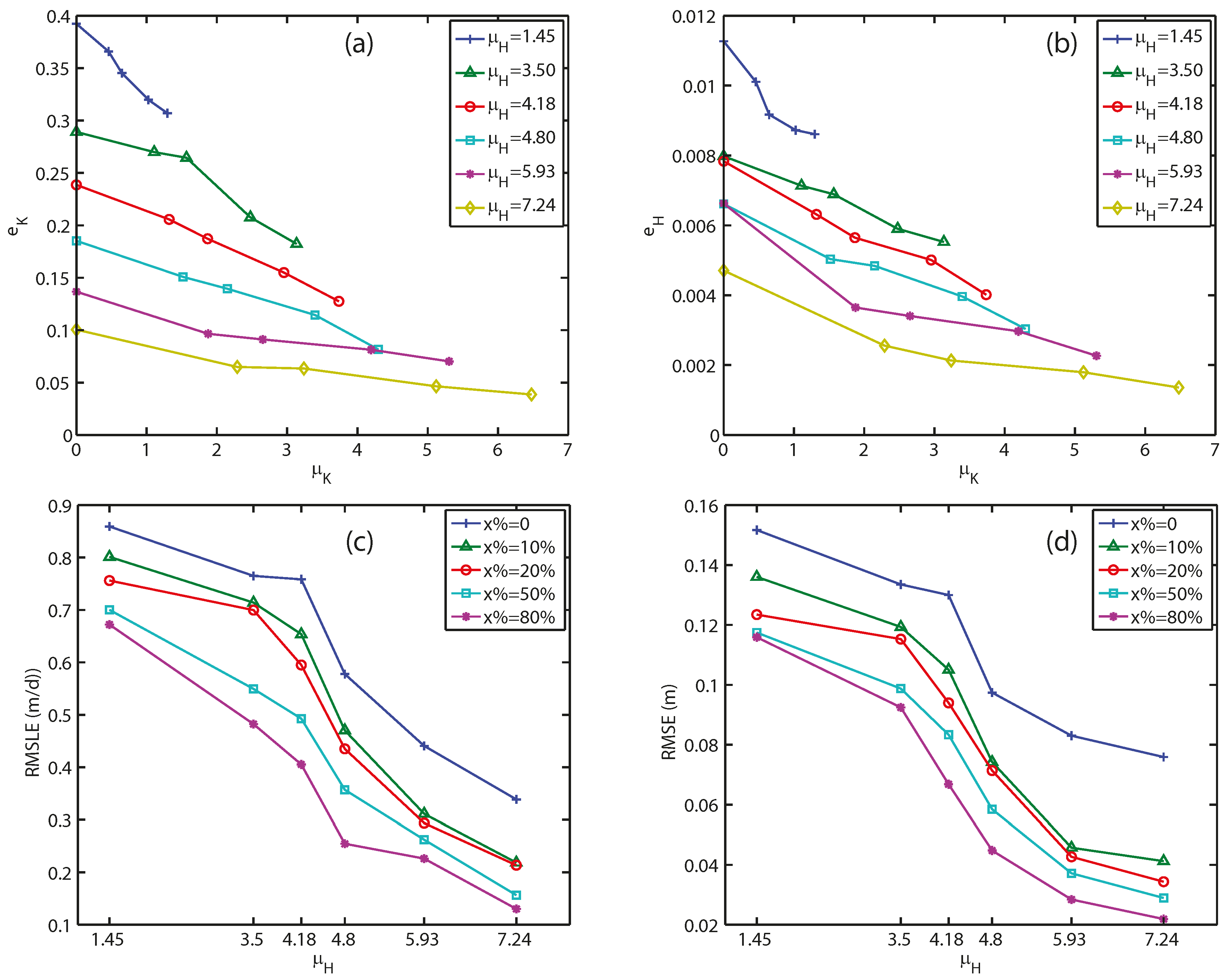
3.3. Errors as a Function of Normalized Data Densities

When we hold ${\mathsf{\mu }}_H$ constant and increase ${\mathsf{\mu }}_K$, $e_K$ gradually decreases as one expects (Figure 5a). The decline in $e_K$ is almost linear. The slopes of the equi-${\mathsf{\mu }}_H$ lines decrease slightly for higher ${\mathsf{\mu }}_H$ values, and the gaps between the lines become smaller at higher ${\mathsf{\mu }}_K$, indicating a moderate interaction between ${\mathsf{\mu }}_K$ and ${\mathsf{\mu }}_H$. The $e_K~{\mu }_K$ curves become flatter when ${\mu }_H$ is higher, suggesting that when ${\mathsf{\mu }}_H$ is higher, the marginal gain attained by the addition of ${\mathsf{\mu }}_K$ decreases. $e_H$ shows a generally similar trend, but there is a more noticeable quadratic trend (Figure 5b).

Toward higher ${\mathsf{\mu }}_K$, we should be able to build a more accurate variogram model for the interpolation procedure during calibration. However, at least in the tested range between ${\mathsf{\mu }}_H$ and ${\mathsf{\mu }}_K$, such a benefit is hardly observable. At the same time, as $e_K$ is computed from comparing “observed” and calibrated K of the entire domain, the monotonously and smoothly varying $e_K$ suggests the regularization approach is effective in reducing overfitting errors.

Viewing the data in a different way, when we keep a constant x%, the error apparently decreases smoothly, as we increase the effective data densities (Figure 5c,d). In this Figure, as ${\mathsf{\mu }}_H$ increases, ${\mathsf{\mu }}_K$ also increases proportionally. When $x\%$ is increased from 0 m to 10%, the reduction of both RMSE and RMSLE are more significant than when it increased from 10% to 20%. As mentioned previously, this pattern is perhaps due to the moderate interaction between ${\mathsf{\mu }}_H$ and ${\mathsf{\mu }}_K$.

3.4. Multivariate Polynomial Curve Fitting

Stepwise multiple regressions show that high-order terms (i.e., the second order) are statistically insignificant for $e_K$ so that the system is mostly linear in the range of tested ${\mathsf{\mu }}_K$ and ${\mathsf{\mu }}_H$ (

Table 1. Multivariate polynomial curve fitting for the following equation: $e\left({\mathsf{\mu }}_H,{\mathsf{\mu }}_K\right)=p_0+p_1{\mathsf{\mu }}_H+p_2{\mathsf{\mu }}_K+p_3{\mathsf{\mu }}_H^2+p_4{\mathsf{\mu }}_K^2+p_5{\mu }_H{\mu }_K$. p-value is the probability of the null hypothesis that the corresponding coefficient is equal to 0 according to the t-statistic.

Calibration Errors		Coefficients in Fitting Equation						Fitting Goodness
		${\mathit{p}}_0$	${\mathit{p}}_1$	${\mathit{p}}_2$	${\mathit{p}}_3$	${\mathit{p}}_4$	${\mathit{p}}_5$	R2	${\mathit{e}}_{\mathit{f}}$
$e_K$	p-Value	0	0	0	0.946	0.697	0	0.975	0.0162
	Value	0.464	−0.0533	−0.061	0	0	0.0075
$e_H$	p-Value	0	0	0	0.939	0.001	0	0.973	0.00043
	Value	0.012	0.0011	−0.00156	0	0	0.00015	−0.982	−0.00035

Note: The p-value of $p_4$ coefficient for $e_H$ is small but still set to be 0. The two values inside the parentheses are the values including the quadratic term ${\mu }_K^2$ when fitting $e_H$.

). The small value of the coefficient for $\left({\mathsf{\mu }}_H,{\mathsf{\mu }}_K\right)$ compared to the other terms confirms that the interaction between the two variables is mild. We created a 3D surface using three terms: ${\mathsf{\mu }}_K$, ${\mathsf{\mu }}_H$, and ${\mathsf{\mu }}_K{\mathsf{\mu }}_H$. Therefore, the final fitted equation can be written as:

$$e\left({\mathsf{\mu }}_H,{\mathsf{\mu }}_K\right)=p_0+p_1{\mathsf{\mu }}_H+p_2{\mathsf{\mu }}_K+p_5{\mu }_H{\mu }_K$$

(14)

where $p_0$ to $p_5$ are fitting parameters contained in P of Equation (9). Meanwhile, the quadratic term, ${\mu }_K^2$, is statistically significant (p-value = 0.001) for $e_H$. However, the R² without the quadratic term is adequately high, and adding the term does not increase it notably. In the interest of parsimony, we chose not to include ${\mu }_K^2$ in the fitted formula for $e_H$ either. As there are no effective dimensionless numbers that characterize $e_H$, we focused on $e_K$.

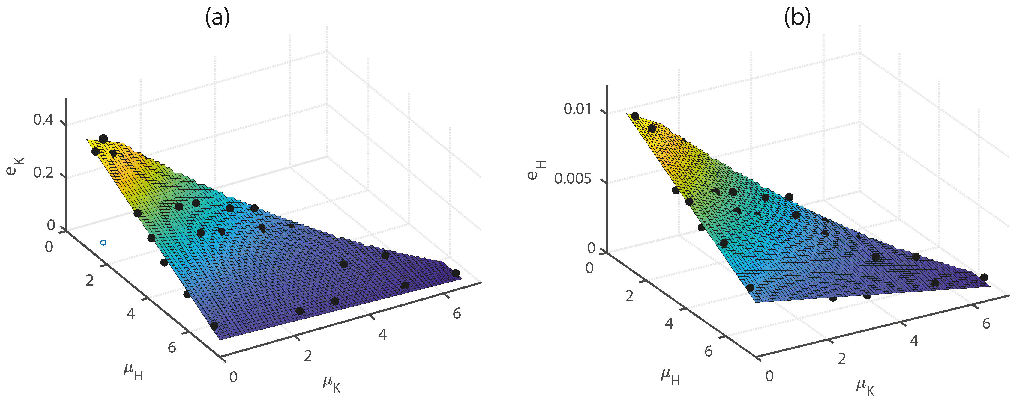
For the first-order terms, the difference between $p_1$ and $p_2$ is~15%. Therefore, in regions where the first-order terms dominate and ${\mathsf{\mu }}_H$ and ${\mathsf{\mu }}_K$ are similar, the data worth of new H and K data points are comparable. This finding suggests, at least across the range tested, groundwater head observations have great value in reducing uncertainties in the K field, and we do not necessarily require knowledge of K values to reduce $e_K$. Also, since $e_K$ is normalized to the range of variability of K, we cannot transfer $e_K$ to dimensionalized uncertainty estimates without some knowledge about the K field. Meanwhile, since $p_1$ and $p_2$ are both negative and $p_5$ is positive, the interaction terms exert a mutually inhibitive effect: The existence of each type of data reduces the marginal benefit of the other type of data. For example, when H observations are dense, because $\frac{\partial e_K}{\partial {\mathsf{\mu }}_K}\approx -0.061+0.0075 {\mathsf{\mu }}_H$, additional K observations do not help as much as when H data density is lower. This almost linear relationship with mutual inhibition is a novel finding. Although we might have an intuitive expectation of an inhibitive relationship, this study is the first to quantitatively determine its relative magnitude.

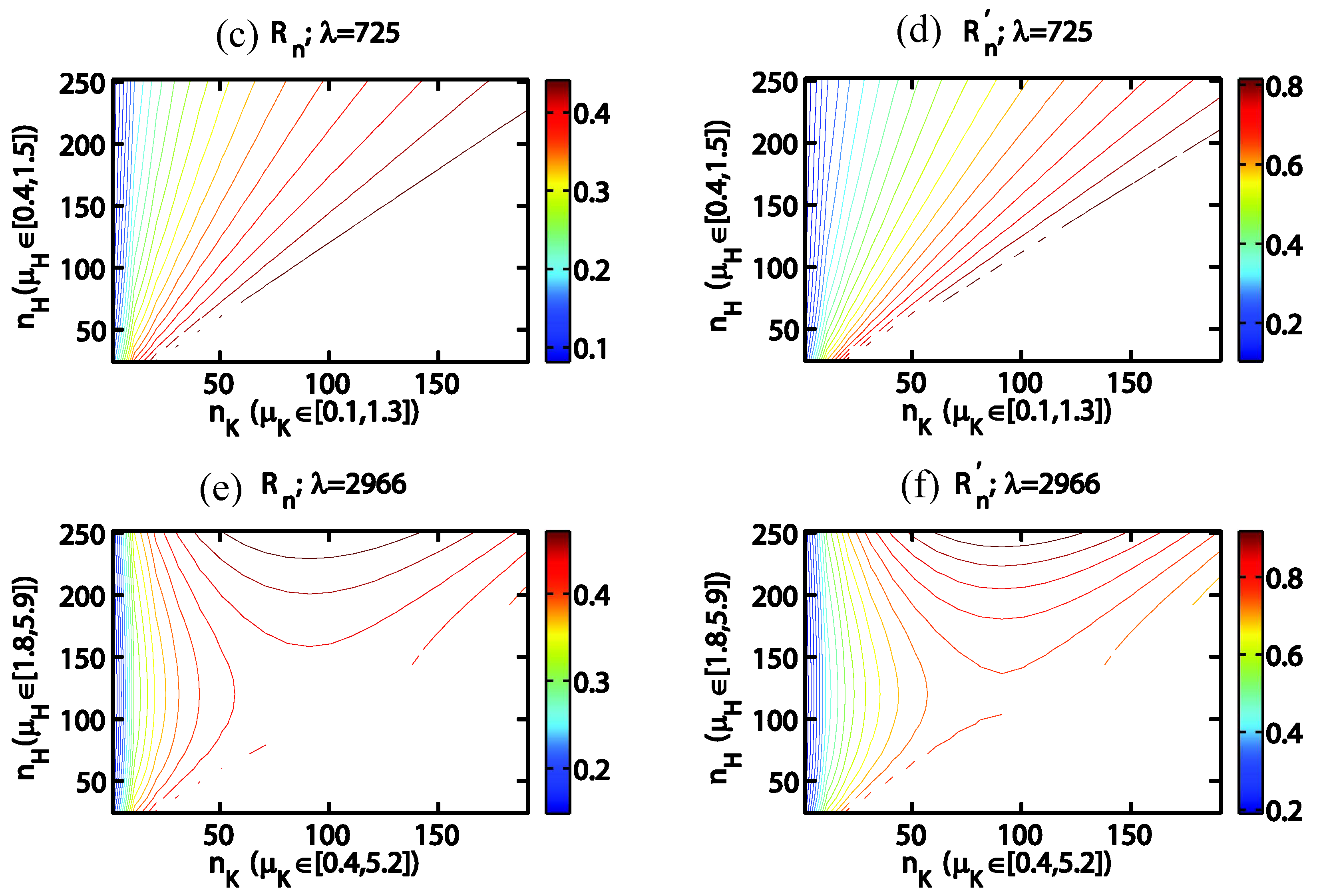
The fitted surface well describes the errors as a function of ${\mathsf{\mu }}_H$ and ${\mathsf{\mu }}_K$ (Figure 6), as most points are scattered closely to the surface. As we assumed ${\mathsf{\mu }}_K$ cannot be greater than ${\mathsf{\mu }}_H$, the valid region is limited to the left lower triangle of the ${\mathsf{\mu }}_H$~${\mathsf{\mu }}_K$ plane. We also provided a contour plot for the surface for a more numerically accurate representation (Figure 7). The contour patterns between $e_H$ and $e_K$ are similar. The contours are denser near the lower left corner, because the gradients of error with respect to $\mathsf{\mu }$s are larger when $\mathsf{\mu }$ is small as a result of smaller mutual inhibition effects.

3.5. Relative Data Value

With either numerical approximation or analytical derivation, we can estimate the ratio between marginal error reduction rates to provide us some insights. For example, $R_{\mu }$ becomes $R_{\mu }\approx \frac{P_1+p_5{\mu }_K}{P_2+p_5{\mu }_H}$, which is clearly a function of both ${\mu }_K$ and ${\mu }_H$. The ${\mu }_K$ tested scatter mostly within the range between 0 to 4.5 (Figure 5). Given a unit increase in the effective data density, H data appears to be more effective in reducing $e_K$ (Figure 8). $R_{\mu }$ is >1 for the greater part of the plane, especially for K error. It rises quickly toward the high ${\mu }_H$, low ${\mu }_K$ region near the upper left corner of the figure. This pattern results from the calculation of $R_{\mu }$: $\mu$ is not a linear function of $n$. To increase one unit in $\mu$ when $\mu$ is high, many data points are required.

$R_n$ is easier to interpret as it shows the ratio of information content brought in by the next data point of H vs. K, but to examine it, we must consider the nonlinear influence of $\lambda$. When $\lambda$ is small (highly heterogeneous field, Figure 8c,d), $R_n$ ranges between 0.1 and 0.8, which means a K data point will always bring in more information content than an H data point. This difference may be counter-intuitive, considering the magnitude of coefficients $p_1$ (−0.053) is only slightly smaller than $p_2$ (−0.061). An important factor is that $n_K$ is always smaller than $n_H$ in our tested ranges, which is normally the case with available groundwater data. $R_n$ contours radiate out almost linearly in the shape of a fan and is dense near the left edge of the figure. The linear pattern of the contours in Figure 8a,b suggest $R_n$ is almost a function of x% for this high-heterogeneity case ($\lambda =725 m$). When $n_K<10$, $R_n<0.1$, meaning K measurement is sparse compared to H, there is 10 times more information value in new K data points than H. However, when $\lambda$ is large (more homogeneous field), we are in a relatively data-rich environment, where the mutual inhibition effect becomes more important. $R_n$ becomes markedly larger and more nonlinear (Figure 8e,f). Toward the left-edge, contours are dense and still mostly vertical. In that region, $R_n$ mainly depends on the amount of K data, and H density has little impact. $R_n$ then increases toward the upper-right corner. If other conditions are equal, new K points bring in more relative value in the small-$\lambda$ case than in the large-$\lambda$ case. As the fraction of K data points increases, new H data points become increasingly useful relative to K.

3.6. The Influence of Noise with K Observations

Although we looked for predictive formulations to describe the relationship between $\beta$ and its three control variables (${\mu }_K$, ${\mu }_H$, ${\mathsf{\sigma }}_n$), we have not been able to find a simple and reliable predictive formulation with $R^2>0.5$. However, we can draw some inferences from our results.

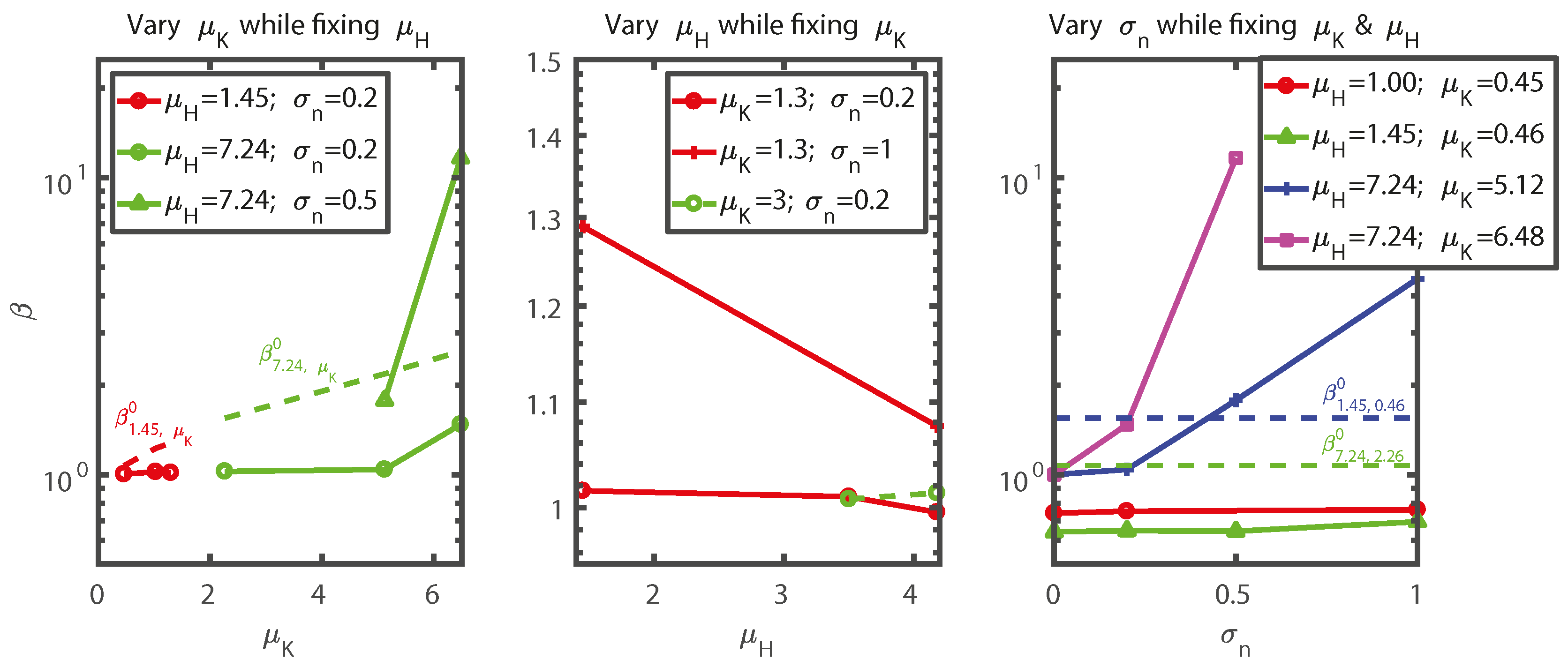
• When ${\mu }_H$ is fixed, $\beta$, in general, grows as a function of increasing ${\mu }_K$ (Figure 9), but when ${\mu }_K<3$, the error amplification is almost close to 1 and $\beta$ is not very sensitive. The largest impact in this category is with the case (${\mu }_K=1.45$, ${\mu }_H=1.3$, ${\mathsf{\sigma }}_n=1$). Recall in this case, 33% of the K data points have been perturbed more than an order of magnitude, but the impact on calibrated K nonetheless appears limited ($\beta =1.29$). However, when ${\mu }_K$ is larger than 3, the errors grow significantly. At (${\mu }_K=6.48$, ${\mu }_H=7.24$, ${\mathsf{\sigma }}_n=0.5$), $\beta =11.6$ (the upper-rightmost point in Figure 9), which means the inversion essentially failed. Another such case is (${\mu }_K=5.12$, ${\mu }_H=7.24$, ${\mathsf{\sigma }}_n=1$) and $\beta =4.57$ (visible in Figure 9 blue line). At (${\mu }_K=6.48$, ${\mu }_H=7.24$, ${\mathsf{\sigma }}_n=0.2$), even if the perturbation is moderate, it still causes a significant error amplification ($\beta =1.47$, the rightmost circle on the lower solid green line).
• Larger ${\mu }_H$ can help inhibit error amplification. When ${\mu }_K$ and ${\mathsf{\sigma }}_n$ are kept the same and ${\mu }_H$ is increased, $\beta$ always decreases. However, this effect is small when ${\mu }_K<3.5$ because the amplification is already small.
• Even though larger ${\mu }_K$ increases the error amplification from a noise-free baseline (Figure 9), incorporating K data points nonetheless reduces error compared to corresponding cases with ${\mu }_K=0$ (note ${\beta }_0$ in Figure 9), as long as ${\mu }_K$ is not too large. For example, under a sparse-data scenario (${\mu }_K=0.45$ or ${\mu }_K=1.3$), even if ${\mathsf{\sigma }}_n=1$, which means significant noise, the error is still less than the case without incorporating K data.
• Under the combined conditions of high ${\mu }_K$ ($>3.5$) (again, this means there are on average 3.5² = 12.25 conductivity data points in an area of ${\lambda }^2$) and high noise (${\mathsf{\sigma }}_n\ge 0.5$), the error amplification skyrockets and dominates over the information content of K. For example, (${\mu }_K=5.1$, ${\mu }_H=7.2$, ${\mathsf{\sigma }}_n=1$), $\beta =4.57$, and $e_K=0.21$ which is greater than the case with the same ${\mu }_H$ but without K data (${\mu }_K=0$). At ${\mu }_K=6.5$ and ${\mu }_H=7.2$, even a ${\mathsf{\sigma }}_n$ of 0.5 is sufficient to bring the error amplification factor to 11.6. For these cases, the errors are too large, and the inversion failed.

Based on these observations, we conclude that, perhaps counter-intuitively, noise with K estimates are more malicious under high ${\mu }_K$ scenarios. When there are only a few K data points, we should incorporate them, even if we know they may have significant noise, provided that the log-standard deviation of that noise is not more than 1 order of magnitude. However, when there are a great number of low-quality K estimates, it is, in fact, better not to use them during the inversion and completely rely on H data. It is possible that the low-quality K has made it very difficult for the inversion process to infer a usable variogram.

4. Conclusions

The main contribution of the paper is to expose the functional form of inverse modeling error as dependent on data densities and the interaction between the density terms for the simplest case. The simple dependence of calibrated K error (but not H error) on the normalized densities have not been shown before. The conclusions of this study, i.e., Equation (14) with coefficients in Table 1, can be applied a priori to roughly estimate the value of groundwater model calibration. For consultants reading others’ works, which resulted from a calibration but without details concerning uncertainty, the formula here can be helpful. We found that the calibrated K error, $e_K$, can be well described by the sum of a linear function of ${\mathsf{\mu }}_H$ and ${\mathsf{\mu }}_K$, and a mild, mutually inhibitive interaction term, which indicates if H density is high, the marginal value of K is reduced and vice versa. This functional form fills a knowledge gap about the value of data and the inversion procedure itself. As the formula is derived in dimensionless forms, it can be applied to various scales and heterogeneity settings. However, the calibrated H error cannot be similarly described by dimensionless numbers. BCs and recharge are found to have little impact on normalized K error. The absolute value of the coefficients of the first-order terms are similar, but relative data worth ratio (H:K) for the next data point, $R_n$, is strongly dependent on the existing data densities. If we assume that a new K observation must entail a new H observation, across most of the tested parameter range, a new H measurement has less than 40% of the data worth of a new K measurement ($R_n<0.4$). When K is sparse, this ratio can be less than 10% ($R_n<0.1$). In a domain with higher heterogeneity, $R_n$ is mostly determined by the fraction of wells with K measurements.

Considering the noise inherent with known K estimates, we should incorporate K data when there are relatively few K data points, or if the data quality is high. Especially, some knowledge about the range of K variability is required to convert the normalized error estimates to ones with units. However, if there are a great number of K data points with low quality, it is, in fact, better not to incorporate them because they make it difficult to estimate a valid variogram.

5. Limitations

The findings help to build a first-order, conceptual understanding, but we must realize real-world situations are far more complex. Certainly, the method employed in this work is simple and empirical. The geometric configuration of the domain and measurement points is simplistic. Therefore, it only represents a rough, a priori estimate, and it needs to be used with caution. More advanced methods should be used to determine the optimum location to place new data points. Finally, our experiments were carried out using the PEST algorithm in the environment of groundwater modeling system software, and the results are, thus, conditioned on some decisions of the program, e.g., the choice of the regularization parameter.