Integrated Real-Time Flood Forecasting and Inundation Analysis in Small–Medium Streams

Abstract

This study presents the application of an adaptive neuro-fuzzy inference system (ANFIS) and one dimensional (1-D) and two dimensional (2-D) hydrodynamic models to improve the problems of hydrological models currently used for flood forecasting in small–medium streams of South Korea. The optimal combination of input variables (e.g., rainfall and water level) in ANFIS was selected based on a statistical analysis of the observed and forecasted values. Two membership functions (MFs) and two ANFIS rules were determined by the subtractive clustering (SC) approach in the processes of training and checking. The developed ANFIS was applied to Jungrang Stream and water levels for six lead times (0.5, 1.0, 1.5, 2.0, 2.5, and 3.0 hour) were forecasted. Based on point forecasted water levels by ANFIS, 1-D section flood forecast and 2-D spatial inundation analysis were carried out. This study demonstrated that the proposed methodology can forecast flooding based only on observed rainfall and water level without extensive physical and topographic data, and can be performed in real-time by integrating point- and section flood forecasting and spatial inundation analysis.

1. Introduction

Since the frequency and scale of damage from torrential rain have increased due to climate change and global warming, flood forecasting has become critical for small–medium streams as well as large rivers. Real-time flood forecasting is always a benchmark problem for hydrologists and water-resource engineers and has received great attention for many decades [1]. Thus, accurate, real-time flood forecasting is vital in flood-prone areas within small–medium watersheds for the issuance of flood warnings to allow lead time for the evacuation of residents and the protection of facilities endangered by imminent rising water levels.

In the past, flood forecasting was mainly performed using conceptual and deterministic models, such as hydrological rainfall-runoff models [2], including deterministic catchment model [3] and geomorphologic instantaneous unit hydrograph (GIUH) model [4]. Such models may require a great deal of work involving field surveying and parameter estimation and a significant amount of calibration to give reliable information for flood forecasting. Additionally, in modeling the relations with rainfall and runoff by using a hydrological model, numerous nonlinear and uncertain elements are implied. Obviously, such models show a lack of practicality and are difficult to use for real-time flood forecasting for small–medium streams in Korea, where watersheds are characterized by high mountains, steep slopes, short travel time, and heavy rainfall during typhoons. In Korea, streams with a watershed area of less than 300 km² and a length of less than 35 km are defined as small–medium streams [5].

However, South Korea still uses the storage function model (SFM), which is one of the rainfall-runoff models, for flood forecasting. Real-time flood forecasting using hydrological rainfall-runoff models requires the calculation of the runoff amount at a specific point and then converting it into water level with a rating curve. Here, the accuracy of flood forecasting depends on the accuracy of the forecasted water level as well as the accuracy of the rainfall-runoff models. However, the accuracy cannot be assured for small–medium streams in Korea because there are many streams where rating curves are not available for various flows. Especially, for small–medium streams, where travel time is short due to their small watershed area, there are greater difficulties in flood forecasting using the hydrological rainfall-runoff models compared to large rivers.

While the data-driven model extracts information of system response to a specific input by constructing a nonlinear function to describe the relationship between input and output data, it does not provide any information on the physics of the hydrological processes. In addition, the data-driven model is usually developed and implemented quickly and easily. Thus, this approach is very useful for real-time flood forecasting for the purpose of obtaining accurate predictions of river flow and water level at specific locations in a timely manner [6].

The neuro-fuzzy approach as a data-driven model has been widely adopted for flood forecasting [7]. A specific approach in neuro-fuzzy development is the ANFIS, which has shown significant results in modeling nonlinear functions. In the ANFIS, the MF parameters are extracted from a data set that describes the system behavior. The ANFIS learns features from the data set and adjusts the system parameters according to a given error criterion. Due to the ability of a neuro-fuzzy system to model complex nonlinear systems, successful applications of this method in water resources modeling have been widely reported for rainfall-runoff simulation [7,8,9,10,11,12,13,14,15,16], river flow forecasting [17,18,19,20,21,22,23], rainfall forecasting [24,25,26,27], and water quality [28,29,30].

The purpose of this study is to construct a real-time flood forecasting and flood analysis system by applying ANFIS, 1-D, and 2-D hydrodynamic models to resolve the problems of hydrological rainfall runoff model currently used for flood forecasting in South Korea. In present practice of Korea, flood forecasts are carried out for each point on the large rivers or small–medium streams. Given the growing concern for flooding on the skirts of river, however, flood forecasting for each river section and spatial inundation analysis in flood prone area are required. Therefore, this study proposed a more reasonable and reliable methodology for integrated flood forecasting and inundation analysis for small–medium streams, and verified the applicability of the methodology by applying it to real-time flood forecasting and inundation analysis of Jungrang Stream, South Korea.

Table 1. The differences between traditional and proposed methods for flood forecasting and inundation analysis.

Classification		Traditional Method	This Study
Focused on		Large river Small–medium stream	Small–medium stream
Model	Hydrological	Physical model (Rainfall-Runoff)	Data-driven model (Neuro-fuzzy)
	Hydrodynamic	1-D river model 2-D inundation model	1-D river model (FLDWAV) 2-D inundation model (FVM)
Flood forecast		Point flood forecasting	Real-time point and section flood forecasting
Inundation		Inundation analysis	Real-time inundation analysis

shows the differences in flood forecasting and inundation analysis between traditional and proposed methods. As shown in Table 1, in the present Korean practice, both point flood forecasting and flood inundation analysis are performed with the rainfall-runoff model and 2-D inundation model, respectively. However, in reality, applying this method to small–medium streams makes it difficult to obtain evacuation time in advance because input data processing time is long and flood propagation time is short. This study showed how to secure evacuation time by linking the point flood forecast of the neuro-fuzzy model based on MATLAB, section flood forecast of 1-D river model (FLDWAV), and spatial inundation analysis of 2-D finite volume model (FVM) to enable real-time flood forecast and inundation analysis in small–medium streams.

2. Methodology

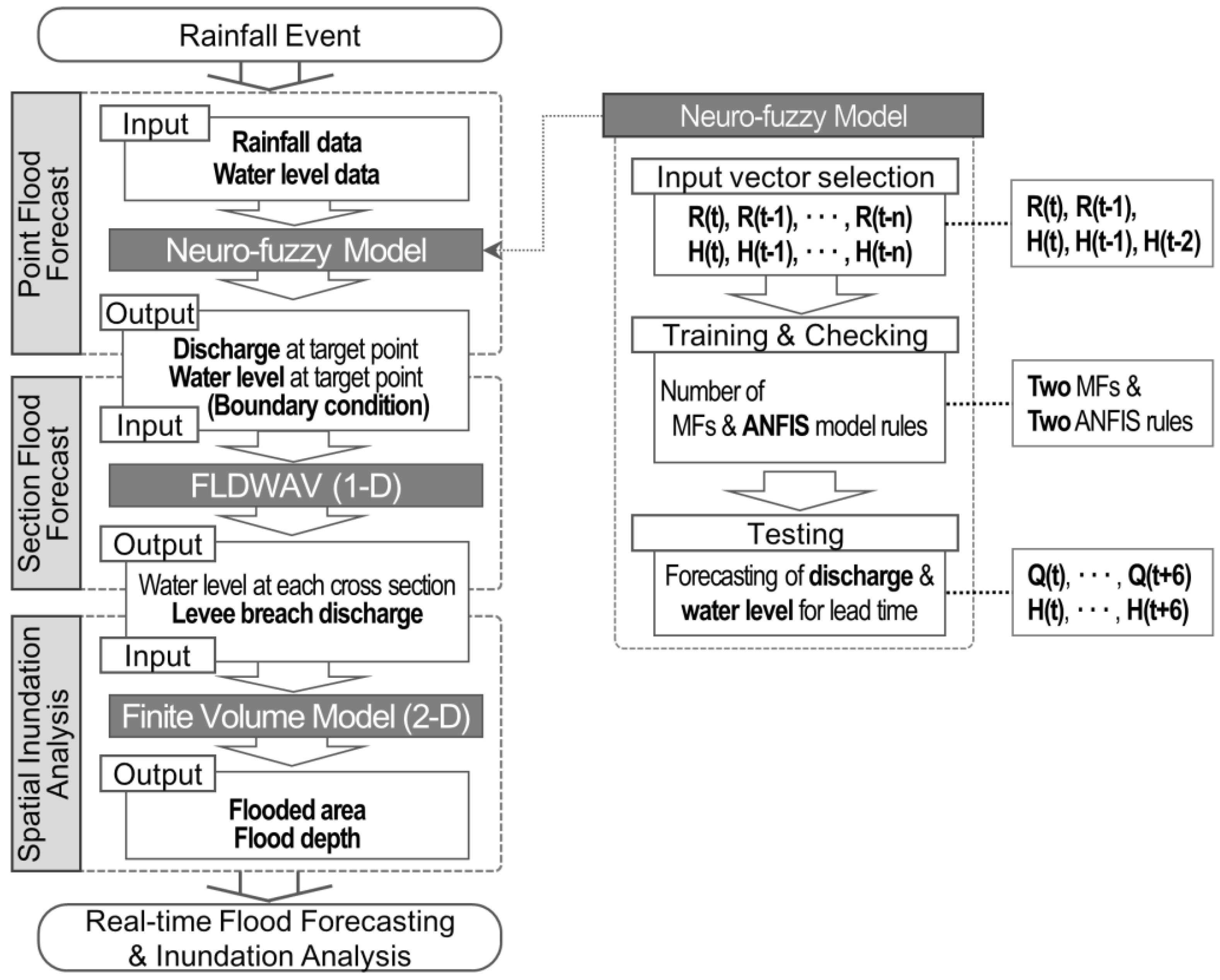
2.1. Method of This Study

This study proposed a methodology for real-time flood forecasting and inundation analysis by developing an ANFIS model and linking it with 1-D and 2-D hydrodynamic models. Figure 1 shows the flow chart of this study. As shown in Figure 1, the input variables and their temporal distribution were selected, and the number of MFs and rules in ANFIS was determined through training and checking process. The discharge and water level at the target point were estimated for each lead time in the testing process, and these data were applied to the boundary conditions of the 1-D river model, resulting in real-time sectional flood forecasting. In particular, since the execution time of the 2-D model greatly depends on the grid size, an appropriate grid resolution was suggested for real-time inundation analysis by comparing the model efficiency (accuracy vs. execution time) according to the grid resolution.

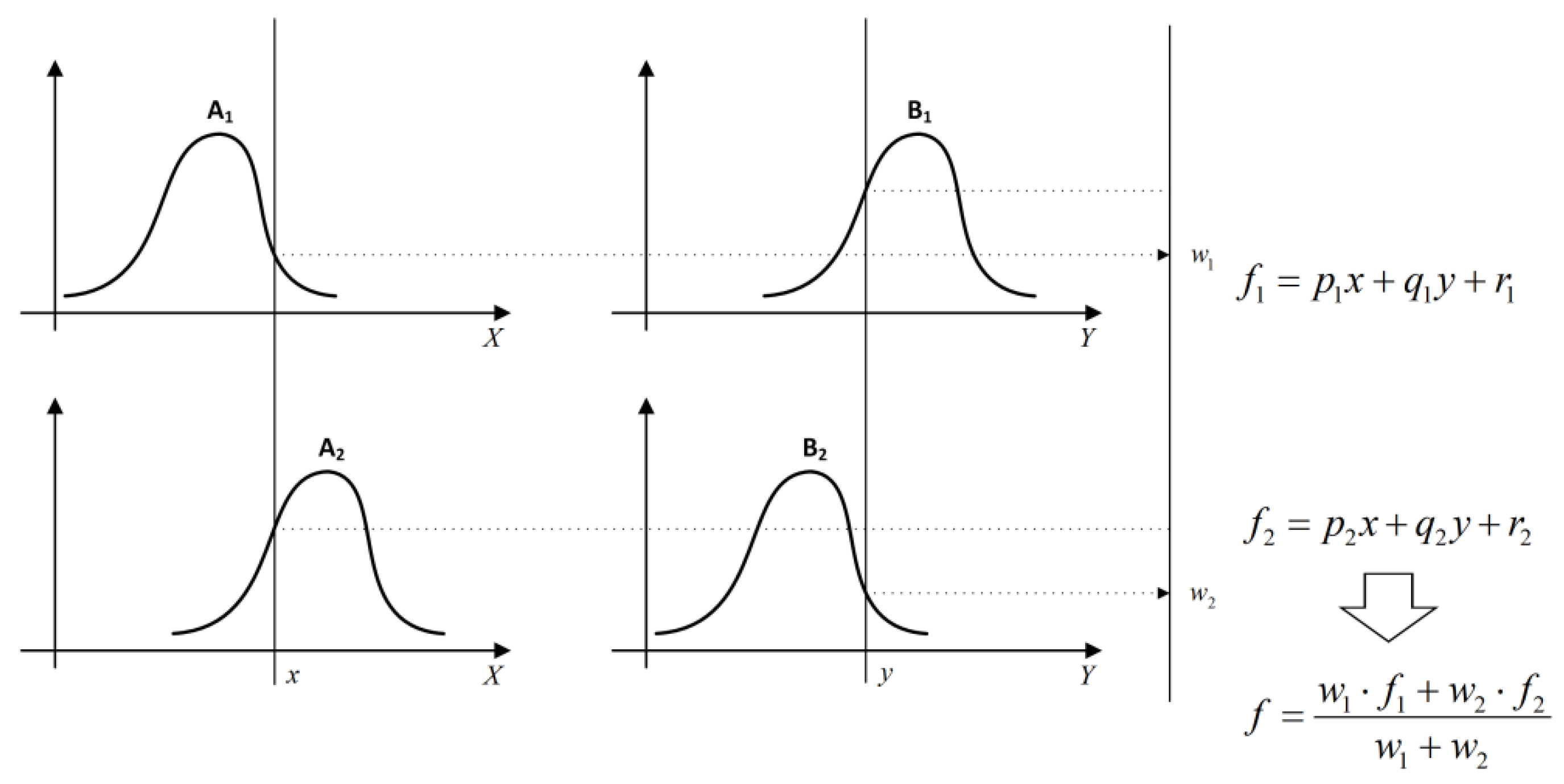
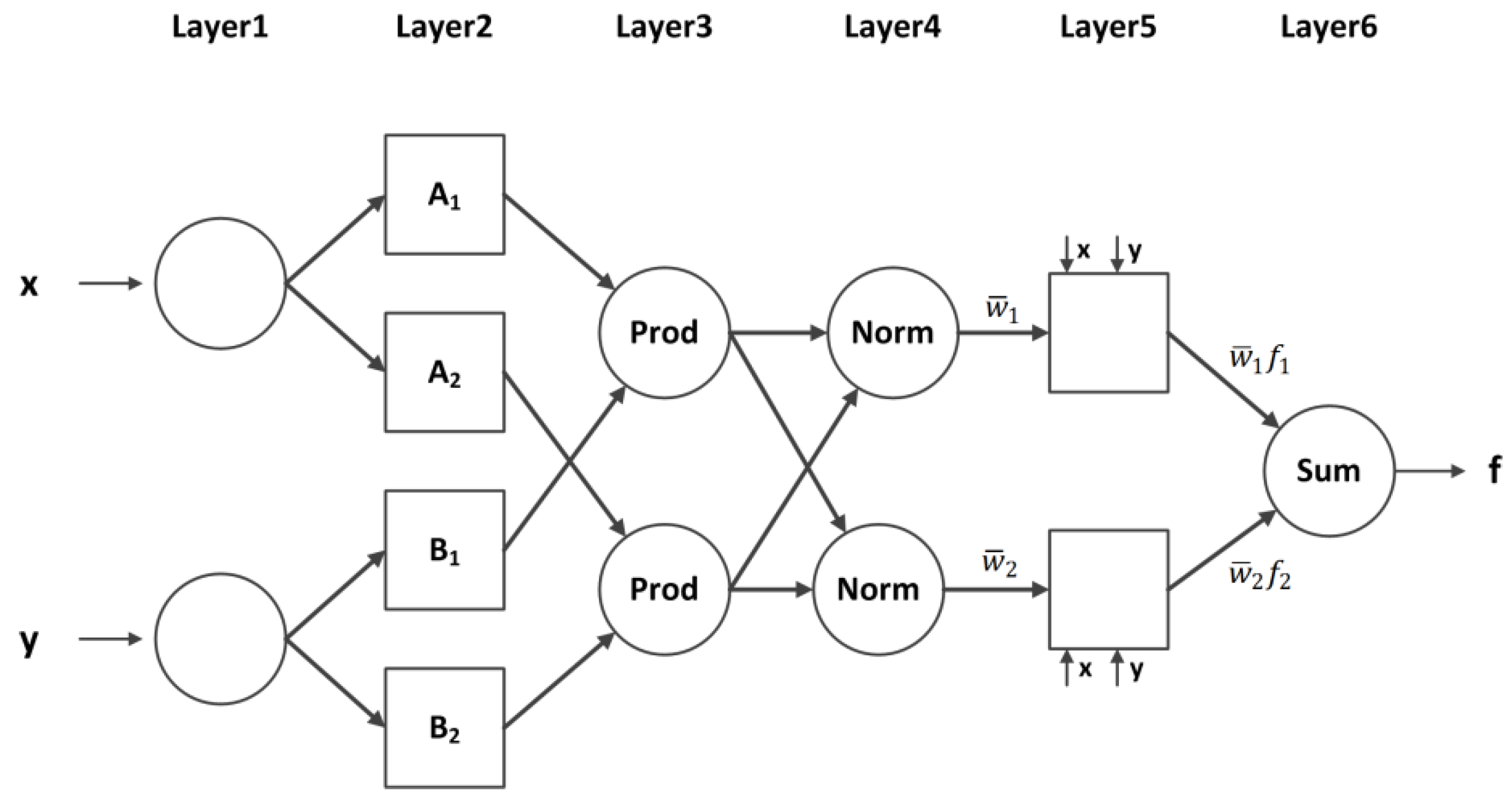
2.2. Adaptive Neuro-Fuzzy Inference System (ANFIS)

ANFIS integrates the advantages of both ANN and fuzzy interference system (FIS). The ANFIS framework is to represent FIS in the ANN structure and optimize the FIS parameters using the learning function of the ANN. Jang [31] proposed the ANFIS and this approach is based on the Takagi–Sugeno–Kang fuzzy inference system [32] embedded within the structure of the ANN [5]. Using a given input-output data set, the ANFIS creates an FIS whose membership function (MF) parameters are adjusted using a back propagation algorithm alone or a combination of a back propagation algorithm with a least squares method. This allows the fuzzy systems to learn from the data being modeled.

To explain the structure of the neuro-fuzzy model of this study, it is assumed that the ANFIS has two inputs, x and $y$, one output, $f$. A first-order Takagi–Sugeno fuzzy model has following two rules:

• Rule 1: If $x$ is $A_1$ and $y$ is $B_1$, then $f_1=p_1+q_1+r_1$
• Rule 2: If $x$ is $A_2$ and $y$ is $B_2$, then $f_2=p_2+q_2+r_2$

where $A_1$, $A_2$ and $B_1$, $B_2$ are the MFs for inputs $x$ and $y$, respectively, and $p_1$, $q_1$, $r_1$ and $p_2$, $q_2$, $r_2$ are the parameters of the output function. Figure 2 illustrates the fuzzy reasoning mechanism for this Takagi–Sugeno model to derive an output function ($f$) from a given input vector ($x$ and $y)$. The structure of ANFIS consists of six layers (Figure 3) and the function of each layer is briefly described as follows:

Layer 1: In this layer, all nodes are inputs and only carry external signals to the next layer.

Layer 2: Every node in this layer is adaptive and generates the membership grades to the input nodes based on the fuzzy set applied membership functions. In this study, Gauss membership function is applied.

Layer 3: This layer contains fixed nodes and generates the firing strength that is the output of this layer by multiplying membership functions obtained in the antecedent layer using an AND operator

Layer 4: This layer named normalized firing strength consists of fixed nodes and computes the ratio of the i-th rule fringe strength

Layer 5: This layer contains the adaptive node and computes the contribution of the i-th rule towards the total output as the product of the normalized firing strength and a first-order Takagi–Sugeno rule.

Layer 6: This layer contains the single node and computes the overall output of the ANFIS as the summation of all incoming signals.

The ANFIS model design consists of two parts: constructing and training. The structure parameters such as the number and type of input and output membership functions are defined in the constructing part. Construction of the ANFIS model requires the partition of the input and output data into rule patches [33]. ANFIS provides three approaches of grid partitioning (GP), subtractive clustering (SC) and fuzzy c-means (FCM) to achieve this partition. In this study, the SC approach was used to partition the data into clusters and determine the minimum number of fuzzy rules and membership functions.

Optimizing the values of adaptive parameters is crucial for improving the performance of adaptive systems. This study used a hybrid learning algorithm [34] to optimize the adaptive parameters in the training part. The hybrid learning algorithm for ANFIS combines two alternating methods, gradient descend and least-squares method. The gradient descend method is used to tune the premise parameters which describe membership functions in layer 2, whereas the least-squares method is used to identify the consequent parameters which describe the coefficients of each output equations in layer 5. The Fuzzy Logic Toolbox of MATLAB was used to implement the ANFIS in this study.

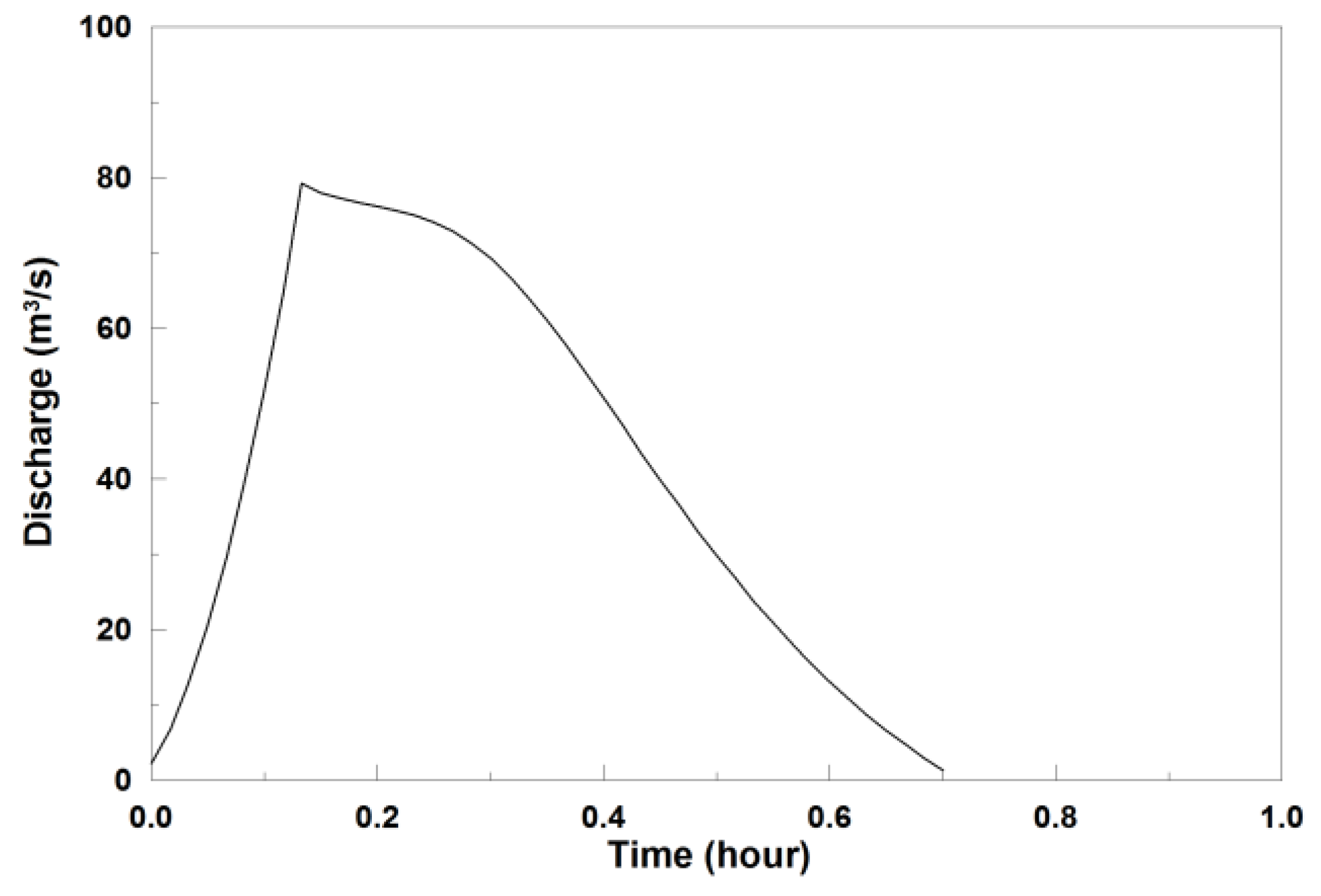
2.3. 1-D Flood Routing Hydrodynamic Model

The Flood Wave (FLDWAV) [35,36] is a generalized unsteady flood routing model in a single river or a system of interconnected waterways. It is based on an implicit finite difference solution of the Saint-Venant equations (SVEs) and the equations express as conservative form of mass and momentum for 1-D open channel flow as follows.

$$\frac{\partial Q}{\partial x}+\frac{\partial \left(A+A_0\right)}{\partial t}-q=0,$$

(1)

$$\frac{\partial Q}{\partial t}+\frac{\partial \left(\beta Q^2/A\right)}{\partial x}+gA\left(\frac{\partial h}{\partial x}+S_f+S_e\right)-\beta q{v}_x+W_{f}B=0,$$

(2)

where, $x$ is a longitudinal distance along the channel or river, $t$ is time, $A$ is cross-sectional area, $A_0$ is cross-sectional area of off-channel dead storage, $q$ is lateral inflow per unit length, $h$ is water surface elevation, $v_x$ is the velocity of lateral flow, $S_f$ is friction slope, $S_e$ is eddy loss slope, $B$ is the width of the channel, $W_f$ is wind shear force, $\beta$ is momentum correction factor, and $g$ is the gravity acceleration.

The Federal Emergency Management Agency (FEMA) has accepted this program for use for National Flood Insurance Program (NFIP) purposes. It can calculate discharges, velocities, depths, and water surface elevations are computed as a function of time and distance along the river [29].

2.4. 2-D Flood Inundation Model

The 2-D Godunov type flood model [37,38,39] was applied to analyze the area where flooding occurred due to levee overflow or failure. This model is based on shallow water equations and can be represented as a conservative form as shown in Equation (3).

$$\frac{\partial U}{\partial \mathit{t}}+\frac{\partial F\left(U\right)}{\partial \mathit{x}}+\frac{\partial G\left(U\right)}{\partial \mathit{y}}=S\left(U\right),$$

(3)

where $U$ is the conservative variable, $F\left(U\right)$ and $G\left(U\right)$ are the flow fluxes in the $x$ and $y$ directions, respectively, and $S\left(U\right)$ is the source term, which consists of the bottom slope and the friction slopes.

In this study, the following two-step fractional method was applied to calculate conservation variables $U_i$ in the grid center at $n+1$ time. In the first step ($n$ and $n^{*}$), fluxes $F\left(U\right)$ and $G\left(U\right)$ are considered (Equation (4a)), and in the second step ($n^{*}$ and $n+1$), $U_i^{n*}$ and $S\left(U\right)$ are considered, thereby calculating conservation variables at the $n+1$ time (Equation (4b)).

$$U_i^{n*}=U_i^n-\frac{\Delta t}{A_i}\left({\displaystyle \sum }_{k=1}^{N_i}{\left(F\cdot n-G\cdot n\right)}_k^n{L}_{i,k}\right),$$

(4a)

$$U_i^{n+1}=U_i^{n*}-\frac{\Delta t}{A_i}{\left(S+Q\right)}_i^{n*},$$

(4b)

where $A_i$ and $N_i$ are the area of i-th grid and the number of interfaces in the grid, respectively, and $L_{i,k}$ is a length of the k-th interface in the grid ($i$).

2.5. Indices of Model Performance

Four different statistical indices were employed to evaluate the model performance. The criteria were computed through comparing the observed data and predicted results. The considered statistical indices are root mean square error (RMSE), correlation coefficient (CC), Nash–Sutcliffe efficiency coefficient (NSEC), and peak relative peak error (RPE). These indices were calculated by the following equations.

$$\mathrm{RMSE}=\sqrt{\frac{\sum {\left(Y_s-Y_f\right)}^2}{n}},$$

(5)

$$\mathrm{CC}=\frac{\sum \left(Y_s-{\overline{Y}}_s\right)\left(Y_f-{\overline{Y}}_f\right)}{\sqrt{\sum {\left(Y_s-{\overline{Y}}_s\right)}^2\times \sum {\left(Y_f-{\overline{Y}}_f\right)}^2}},$$

(6)

$$\mathrm{NSEC}=1-\frac{\sum {\left(Y_s-Y_f\right)}^2}{\sum {\left(Y_s-{\overline{Y}}_f\right)}^2},$$

(7)

$$\mathrm{RPE}=\frac{\left|Y_{s.peak}-Y_{f.peak}\right|}{Y_{s.peak}}\times 100(\%),$$

(8)

where $n$ is the number of data points, $Y_s$ and $Y_f$ are the observed and forecasted value, respectively. ${\overline{Y}}_s$ and ${\overline{Y}}_f$ represent the mean value, respectively and $Y_{s.peak}$ and $Y_{f.peak}$ represent the peak value, respectively.

3. Study Area and Data Selection

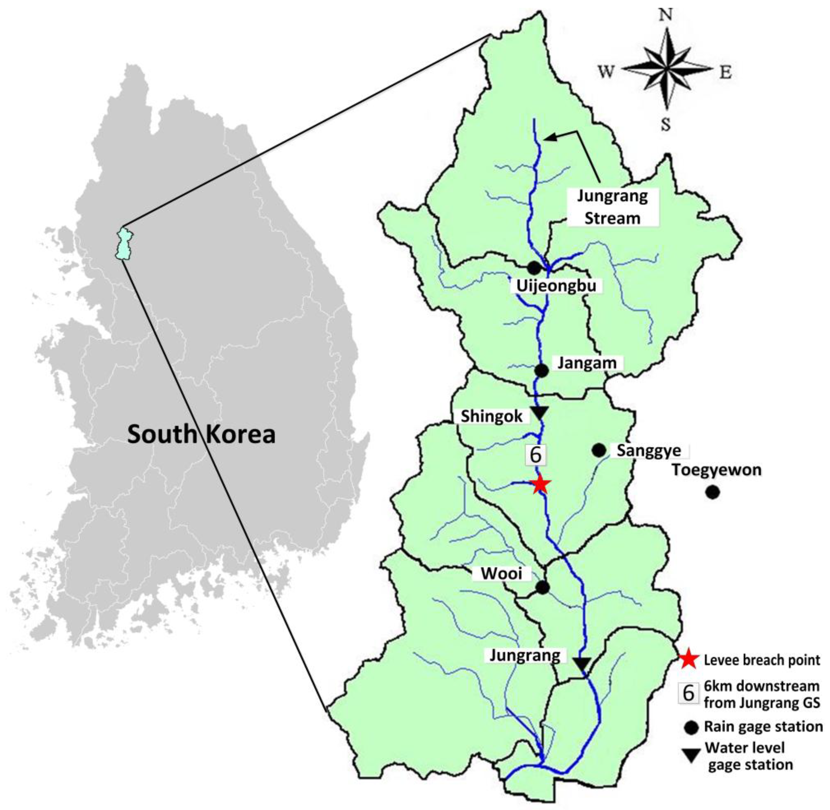
3.1. Study Aarea

The models were applied to the Jungrang Stream in the Han River basin, South Korea. The Jungrang Stream is 296.04 km² in watershed area, 34.8 km in length, 8.1 m in average width, and 1/1150 in average bed slope [5]. The study area and the location of gauge stations are shown in Figure 4. Water level data was obtained from two gauge stations located on the Jungrang Stream, and rainfall record data was obtained from five automatic weather stations (AWS) near the study area (Figure 4).

Table 2. Rainfall events for input vector selection, training, checking, and testing processes.

Event	Start Time	Duration (h)	Total Rainfall (mm)	Cause	Process
J-1	29 Apr. 2002 08:00	32.0	81.1	Low pressure	Testing
J-2	5 Jul. 2002 09:30	38.5	94.7	Typhoon	Testing
J-3	4 Aug. 2002 07:00	88.0	361.3	Low pressure	Input vector selection
J-4	5 Jun. 2003 14:00	32.0	96.4	Low pressure	Training
J-5	21 Jul. 2003 19:00	37.0	192.1	Seasonal rain front	Testing
J-6	6 Aug. 2003 11:00	20.5	65.9	Low pressure	Testing
J-7	19 Aug. 2003 14:00	23.0	149.8	Low pressure	Testing
J-8	23 Aug. 2003 04:30	122.5	319.8	Low pressure	Checking
J-9	18 Sept. 2003 04:00	20.0	142.4	Low pressure	Testing
J-10	3 Jul. 2004 18:30	40.0	83.7	Low pressure	Testing
J-11	11 Jul. 2004 18:30	36.5	138.9	Low pressure	Testing
J-12	26 Jun. 2005 17:00	25.5	136.3	Low pressure	Testing
J-13	1 Jul. 2005 00:30	62.5	118.3	Seasonal rain front	Testing
J-14	28 Jul. 2005 00:30	17.5	122.9	Low pressure	Input vector selection
J-15	10 Aug. 2005 09:00	49.0	112.9	Low pressure	Testing
J-16	24 Aug. 2005 21:00	23.0	83.0	Low pressure	Testing
J-17	13 Sept. 2005 05:30	18.0	95.6	Low pressure	Testing

presents the seventeen rainfall events to examine the neuro-fuzzy system performance in the study area.

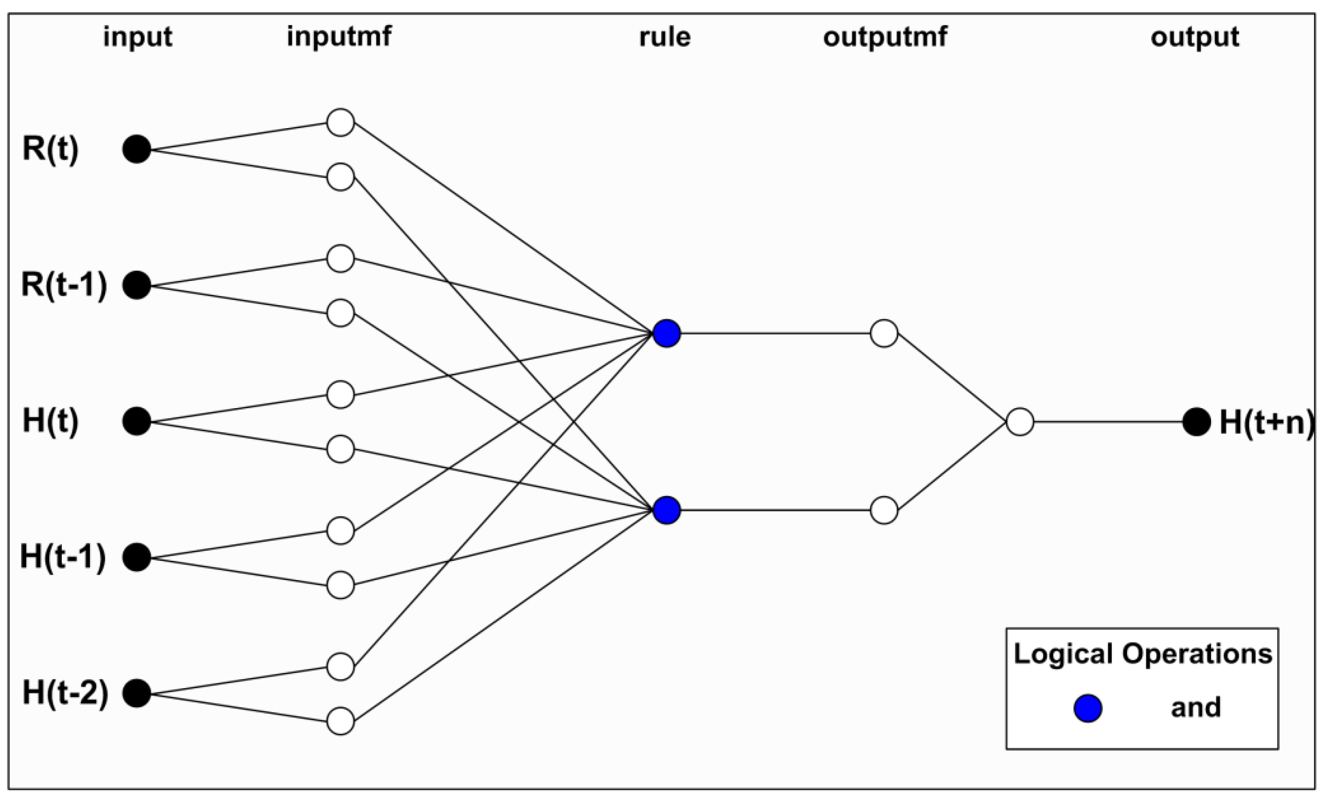
3.2. Input Vector Selection

3.2.1. Model Set-Up

An appropriate input vector selection to find the relevant factors that have an influence on the output is one of the most important tasks in developing a successful forecast of a data-driven model [40]. In this study, in order to select the optimal combination of input vectors, six ANFIS models using measured rainfall and water level were set up as shown in

Table 3. Six ANFIS model and corresponding input vectors.

Model	Combination Code	Input Variable
		Rainfall	Water Level
M-1	H01234	-	H(t), H(t-1), H(t-2), H(t-3), H(t-4)
M-2	R0_H0123	R(t)	H(t), H(t-1), H(t-2), H(t-3)
M-3	R01_H012	R(t), R(t-1)	H(t), H(t-1), H(t-2)
M-4	R012_H01	R(t), R(t-1), R(t-2)	H(t), H(t-1)
M-5	R0123_H0	R(t), R(t-1), R(t-2), R(t-3)	H(t)
M-6	R01234	R(t), R(t-1), R(t-2), R(t-3), R(t-4)	-

. The number of input vectors in six models was limited to five to reduce the processing time. In Table 3, H and R represent the water level and rainfall, respectively, and the number in parentheses indicates the time step of the input vector; e.g., “0” means current time and “-1” means one time step earlier than current time. That is, one time step is 0.5 hour which is the same as the measurement time interval of water level and rainfall, and H(t-2) means the water level at 1.0 hour before the current time.

The six models were applied to J-3 and J-14 events to estimate the water level of 30 min lead time, and the optimal model was selected based on the quantitative results of statistical indices analyzed by comparing observed and estimated values (

Table 4. Quantitative analysis of statistical indices for six ANFIS models.

Event	Model	Model Performance Index
		RMSE (cm)	CC	NSEC	RPE
J-3	M-1	1.32	1.00	0.99	2.42
	M-2	2.33	1.00	0.98	2.87
	M-3	0.76	1.00	1.00	1.45
	M-4	1.48	1.00	0.99	2.63
	M-5	1.94	1.00	0.99	1.78
	M-6	56.47	−0.26	−9.60	65.83
J-14	M-1	8.44	0.99	0.98	3.36
	M-2	6.8	0.99	0.99	4.22
	M-3	4.97	1.00	0.99	0.58
	M-4	7.33	0.99	0.99	3.46
	M-5	9.08	0.99	0.98	11.22
	M-6	77.85	−0.06	−0.39	1.71

). As shown in Table 4, the RMSE of all models except M-6 was less than 0.1 m and CC of those is higher than 0.99. In other statistical indices, the difference of values between models, except M-6, was not large. The RMSE of the M-3 was about 31~74% smaller than other models, and other statistical indices also present the best results at M-3. Based on the quantitative analysis of statistical indices, this study selected M-3 as the optimal input combination for real-time flood forecasting.

3.2.2. Parameter Estimation of the Neuro-Fuzzy Model

In order to examine the applicability of the neuro-fuzzy model, three processes of training, checking, and testing were performed and the parameters of the MF were determined in the processes of training and checking. The parameter values of the MF vary depending on the rainfall events used in the training and checking process, and thus rainfall obviously led to the difference of the neuro-fuzzy model results. In this study, J-3 and J-14 were applied to the selection of optimal input data, and J-4 and J-8 were used for training and checking, respectively, and the remaining thirteen rainfalls among seventeen rainfall events (Table 2) were applied for testing.

In applying the neuro-fuzzy system, more numbers of input variables do not necessarily lead to proportionally more accurate results from the model. In fact, this may result in a long execution time due to exponentially more fuzzy rules. If a neuro-fuzzy model has $\mathrm{n}$ input variables and each input variable has two rules, the total number of rules is 2ⁿ; e.g., if there are five input variables and each variables has two rules (the minimum number of rules is two in the neuro-fuzzy model), the model has 2⁵(=32) rules in total.

In this study, the numbers of MFs and ANFIS model rules were determined by using the SC approach, which is one of the fuzzy clustering methods for input data, in order to shorten the execution time and optimize the input space partitioning. The SC parameters were manually calibrated and the combination of “A (Range of influence)” = 0.5, “B (Accept ratio)” = 0.5, “C (Reject ratio)” = 0.2, and “D (Number of MF)” = 2 showing the smallest training and checking error was applied as an optimal values of each parameter. In addition, a Gaussian function was used as the shape of MF considering the nonlinearity of input (water level and rainfall) and output data (water level). In summary, this study used the M-3 ANFIS model with two MFs and two rules for each input variable as shown in Figure 5.

4. Application

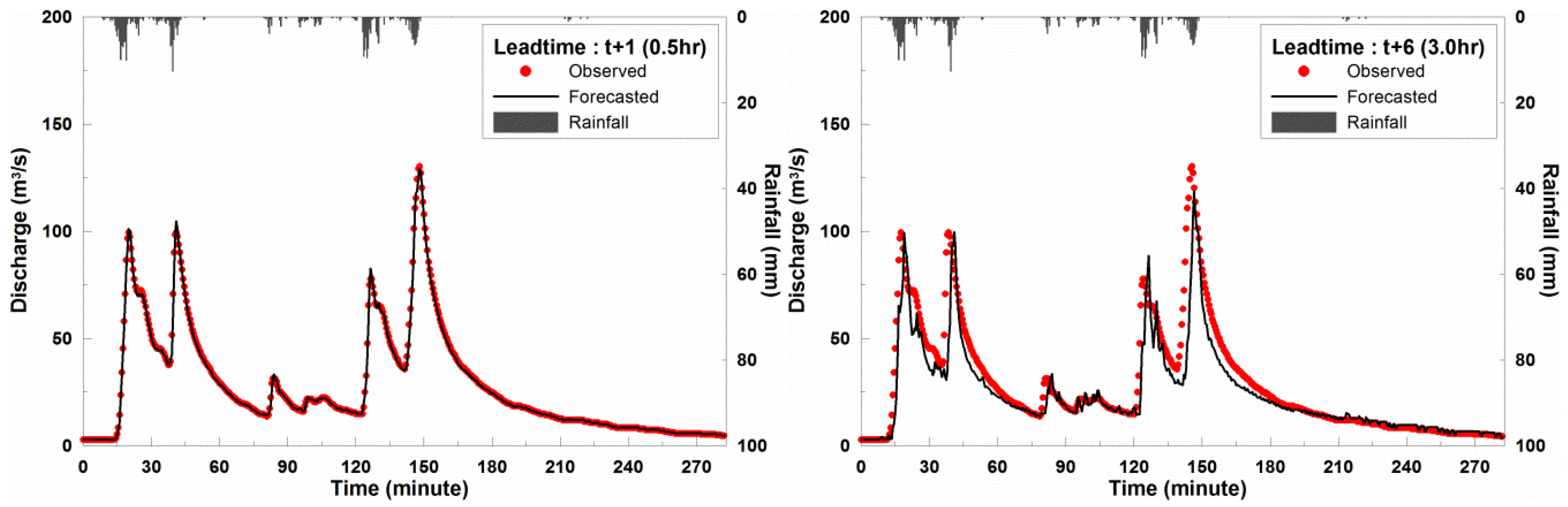
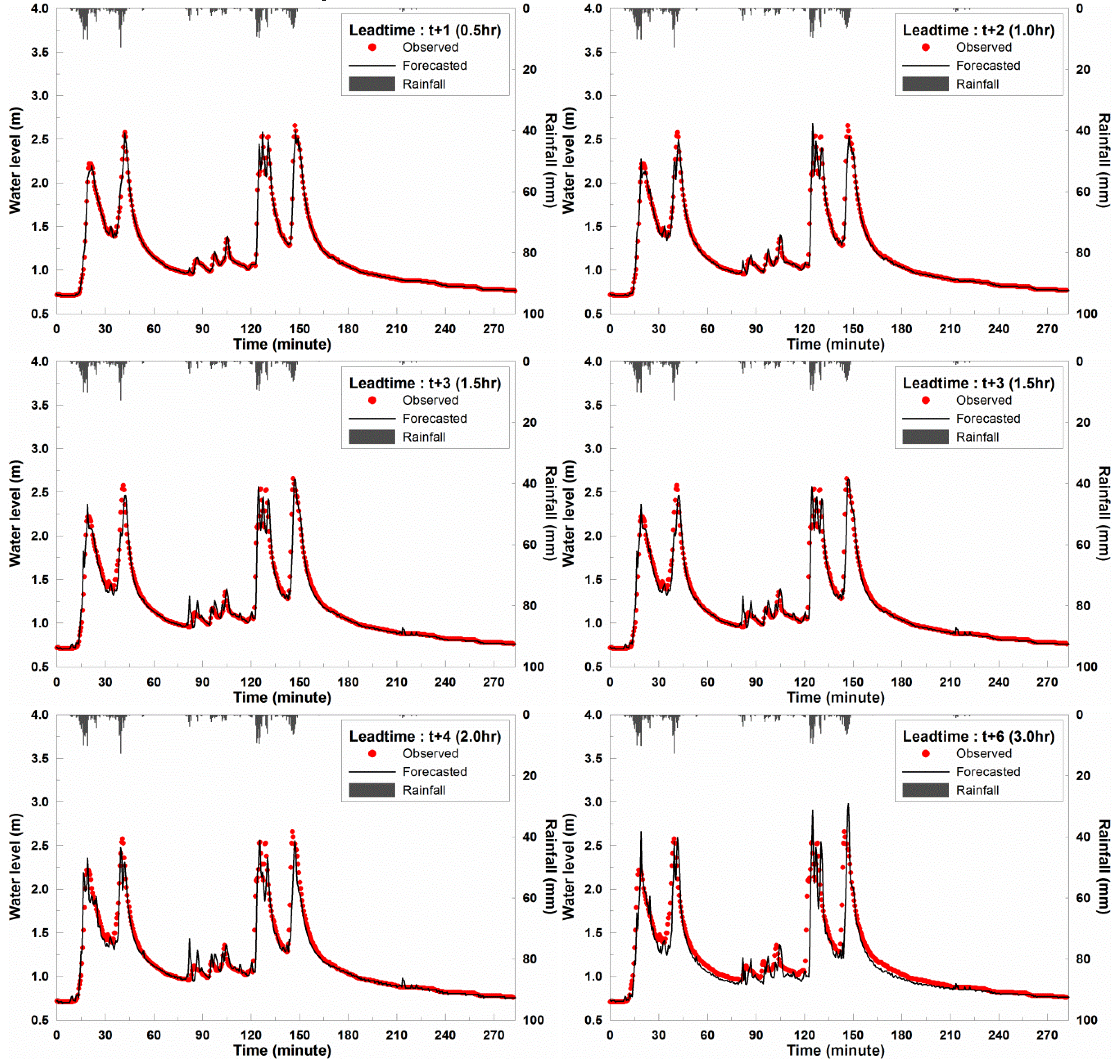
4.1. Real-Time Point Flood Forecasting

The training, checking, and testing processes of the ANFIS were performed for two gauge stations (Jungrang and Shingok), respectively. The training and checking processes were already described in Section 3.2.2, and the model performance indices calculated in each process are shown in

Table 5. Performance indices of ANFIS model for real-time flood forecasting.

Process	Gauge Station	RMSE (Jungrang: m, Shingok: m3/s)						NSEC
		t+1 (0.5 h)	t+2 (1.0 h)	t+3 (1.5 h)	t+4 (2.0 h)	t+5 (2.5 h)	t+6 (3.0 h)	t+1 (0.5 h)	t+2 (1.0 h)	t+3 (1.5 h)	t+4 (2.0 h)	t+5 (2.5 h)	t+6 (3.0 h)
Training	Jungrang	0.01	0.02	0.03	0.04	0.06	0.09	1.00	1.00	0.99	0.99	0.98	0.94
	Shingok	0.26	0.47	0.73	1.11	1.56	2.03	1.00	1.00	1.00	0.99	0.99	0.98
Checking	Jungrang	0.06	0.12	0.17	0.19	0.22	0.27	0.99	0.96	0.93	0.90	0.87	0.81
	Shingok	2.03	2.81	4.33	6.25	8.70	11.53	1.00	0.99	0.98	0.96	0.92	0.85
Testing	Jungrang	0.04	0.07	0.11	0.13	0.16	0.20	0.99	0.97	0.94	0.89	0.84	0.77
	Shingok	2.17	3.78	5.42	6.97	8.38	9.84	0.99	0.97	0.94	0.90	0.86	0.80
Process	Gauge Station	CC						RPE (%)
		t+1 (0.5 h)	t+2 (1.0 h)	t+3 (1.5 h)	t+4 (2.0 h)	t+5 (2.5 h)	t+6 (3.0 h)	t+1 (0.5 h)	t+2 (1.0 h)	t+3 (1.5 h)	t+4 (2.0 h)	t+5 (2.5 h)	t+6 (3.0 h)
Training	Jungrang	1.00	1.00	1.00	0.99	0.99	0.97	0.21	0.24	0.01	0.68	0.50	6.66
	Shingok	1.00	1.00	1.00	1.00	0.99	0.99	0.13	0.17	1.33	1.94	3.15	4.36
Checking	Jungrang	1.00	0.98	0.96	0.96	0.94	0.91	0.60	4.41	5.86	6.24	5.29	5.96
	Shingok	1.00	1.00	0.99	0.98	0.96	0.93	0.98	2.62	1.01	1.99	2.79	3.66
Testing	Jungrang	1.00	0.99	0.97	0.95	0.92	0.89	1.43	3.46	3.84	5.23	8.25	9.98
	Shingok	1.00	0.99	0.97	0.96	0.94	0.91	1.52	2.67	3.14	4.41	6.50	9.73

. Section 4.1 describes the testing process in three phases.

The selected M-3 ANFIS model was applied to thirteen rainfall events (excluding four events, applied to input vector selection, training, and checking) for the testing process, and flood forecasting for the six leading times (0.5, 1.0, 1.5, 2.0, 2.5, and 3.0 hour) was carried out for each event in the Jungrang gauge station (GS). Figure 6 shows a comparison of the forecasted water level and observation for each lead time of J-11 event. Among the thirteen rainfall events applied in this study, only the J-11 event (related to Section 4.3) that resulted in urban flooding due to levee breach was illustrated. As shown in Figure 6, the forecasts were well matched with observations up to 2.0 hour lead time. At the lead times of 2.5 and 3.0 hour, the two values (forecasts and observations) were in agreement with each other overall, but the forecasts are slightly delayed from the observations at the part where the water level is rising. In the case of the peak water level, the forecasts and observations were almost identical until the 2.0 hour leading time, but the forecasts were somewhat higher than the observations at the leading times of 2.5 and 3.0 hour.

For the quantitative analysis of flood forecasting by the model, model performance indices (RMSE, CC, NSEC, and RPE) were investigated. The single rainfall events of J-4 and J-8 were applied to the training and checking processes, respectively, whereas thirteen rainfall events were applied in the testing process (Table 2) and the average values of model performance indices are shown in Table 5.

The average of all events in the RMSE was 0.04 m at 0.5 hour, 0.11 m at 1.5 hour, and 0.20 m at 3.0 hour lead time, respectively. RMSE gradually increased as lead time increased, but overall it was fairly accurate. The average of all events in NSEC was 0.94 at 1.5 hour, 0.84 at 2.5 hour, and 0.77 at 3.0 hour lead time, respectively. As with the RMSE, the NSEC tended to decrease as lead time increased. The CC between the observed and the forecasted water level showed 0.99 at 1.0 hour and 0.92 at 2.50 hour lead time. The mean CC was close to 1.0 for 0.5 hour, 0.95 for 2.0 hour, and 0.89 for 3.0 hour, showing a high correlation between the forecasted water level and the observation. The mean RPE is 1.4% at 0.5 hour, 3.5% at 1.5 hour and 5.2% at 2.0 hour lead time. Even with 3.0 hour lead time, the mean RPE is less than 10%, showing that the observed peak values were well matched with those forecasted by the neuro-fuzzy model.

These statistical indices for each lead time presented that flood forecasting by the neuro-fuzzy model was fairly accurate for up to 3 hour lead time even if the accuracy diminished as the lead time increased.

The water levels for each lead time at Jungrang GS were already forecasted (Figure 6), and these were imposed as the downstream boundary conditions for 1-D hydraulic model. To obtain the water level at Shingok GS for the upstream boundary condition of 1-D model, an additional neuro-fuzzy model was conducted as the same method shown in Jungrang GS. Then, the forecasted water level was converted to discharge using a rating-curve (http://www.hrfco.go.kr/) for the upstream boundary condition. To forecast the water level at Shingok GS, additional neuro-fuzzy model was conducted as the same method shown at Jungrang GS. Then, the forecasted water level was converted into the discharge using a rating-curve (http://www.hrfco.go.kr/). The reason for converting the forecasted water level into the discharge was to apply it as the upstream boundary condition of the 1-D hydrodynamic model. In general, the discharge and water level are applied to the upstream and downstream boundary conditions, respectively, in the hydrodynamic model. At the Shingok GS, the water level is observed, while the discharge is not observed and converted from the observed water level using a rating curve. Thus, the forecasted water level from ANFIS using observed water level and rainfall was converted into the discharge.

Figure 7 presents the converted discharge for t+1 (0.5 hour) and t+6 (3.0 hour) among six lead times in the J-11 event at Shingok GS. This figure also shows a comparison of the two discharges converted from the observed and forecasted water level at Shingok GS. The forecasted discharge (Figure 7) and water level (Figure 6) were applied to 1-D hydrodynamic model as the upstream and downstream boundary conditions, respectively. The model performance indices for the ANFIS testing process at Shingok gauge station are shown in Table 5. As shown in Table 5, it showed better results than the Jungrang gauge station.

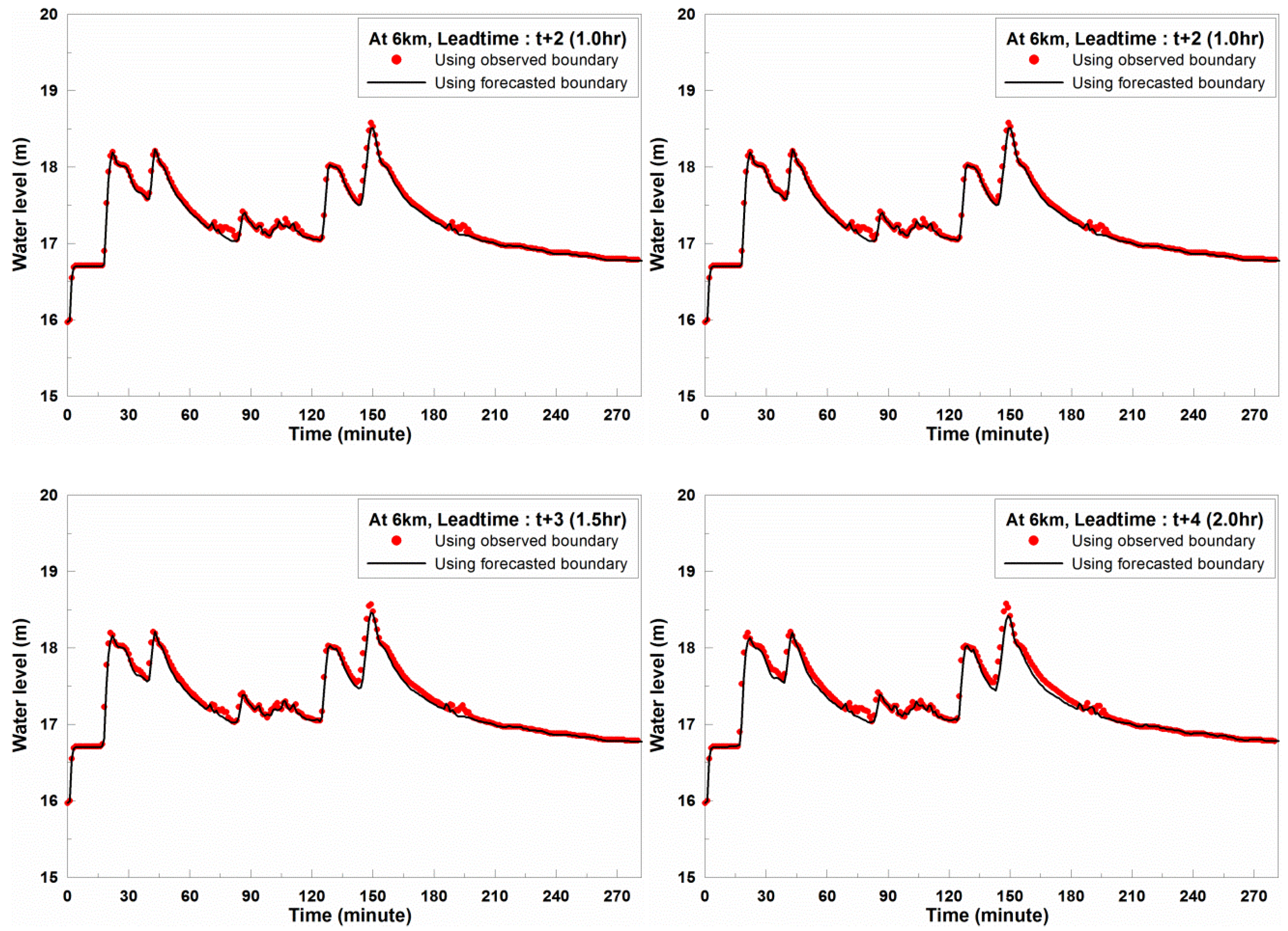
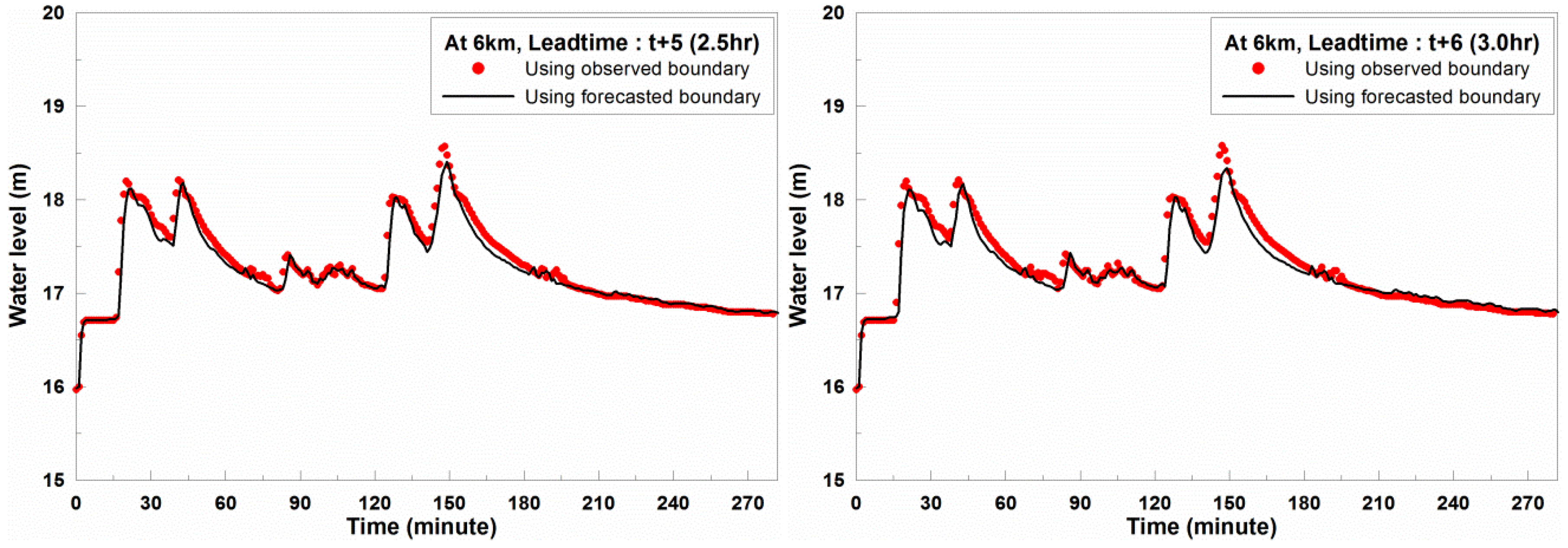
4.2. Real-Time Section Flood Forecasting

The FLDWAV, a 1-D river analysis model, was applied to the section of Shingok GS and Jungrang GS in the study area (Figure 4) by imposing the forecasted discharge and water level as the upstream and downstream boundary conditions.

To validate the model, predicted water levels from the 1-D hydraulic model using forecasted boundary conditions were compared with predicted ones using the observed boundary conditions. Figure 8 presents the comparisons between two predictions at 6 km downstream from the Jungrang G

S for each lead time of J-11 event. When the lead times were 0.5, 1.0, and 1.5 h, the predicted water levels from forecasted and observed boundary conditions are well agreed, and peak water level and its occurrence time were also well matched. The RMSEs were 1.5, 5.3, and 11.6 cm for the lead times of 0.5, 1.0, and 1.5 h, respectively, and it is slightly increased from 2.0 hour lead time. The RMSEs were increased to 16.1, 19.7, and 21.5 cm at the lead times of 2.0, 2.5, and 3.0 h, respectively. Although the difference between two predictions increased somewhat from the 2.0 hour lead time, overall there was good agreement. The results of 1-D river modeling of this study showed that the predictions using the boundary condition forecasted by the neuro-fuzzy model were in agreement with those using the observed boundary condition. This indicated the applicability of the neuro-fuzzy forecast model for real-time river analysis to forecast floods.

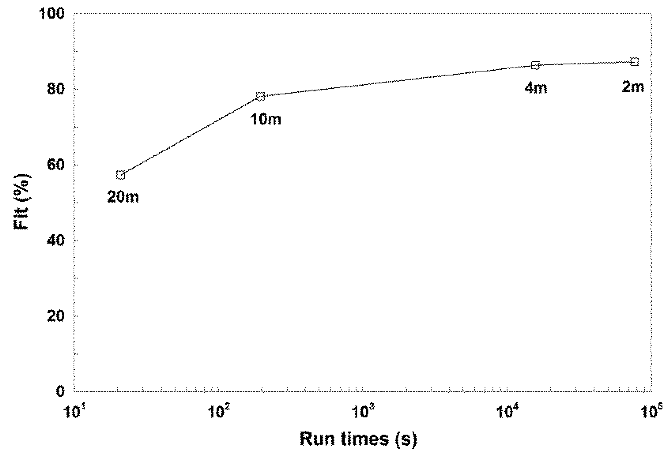
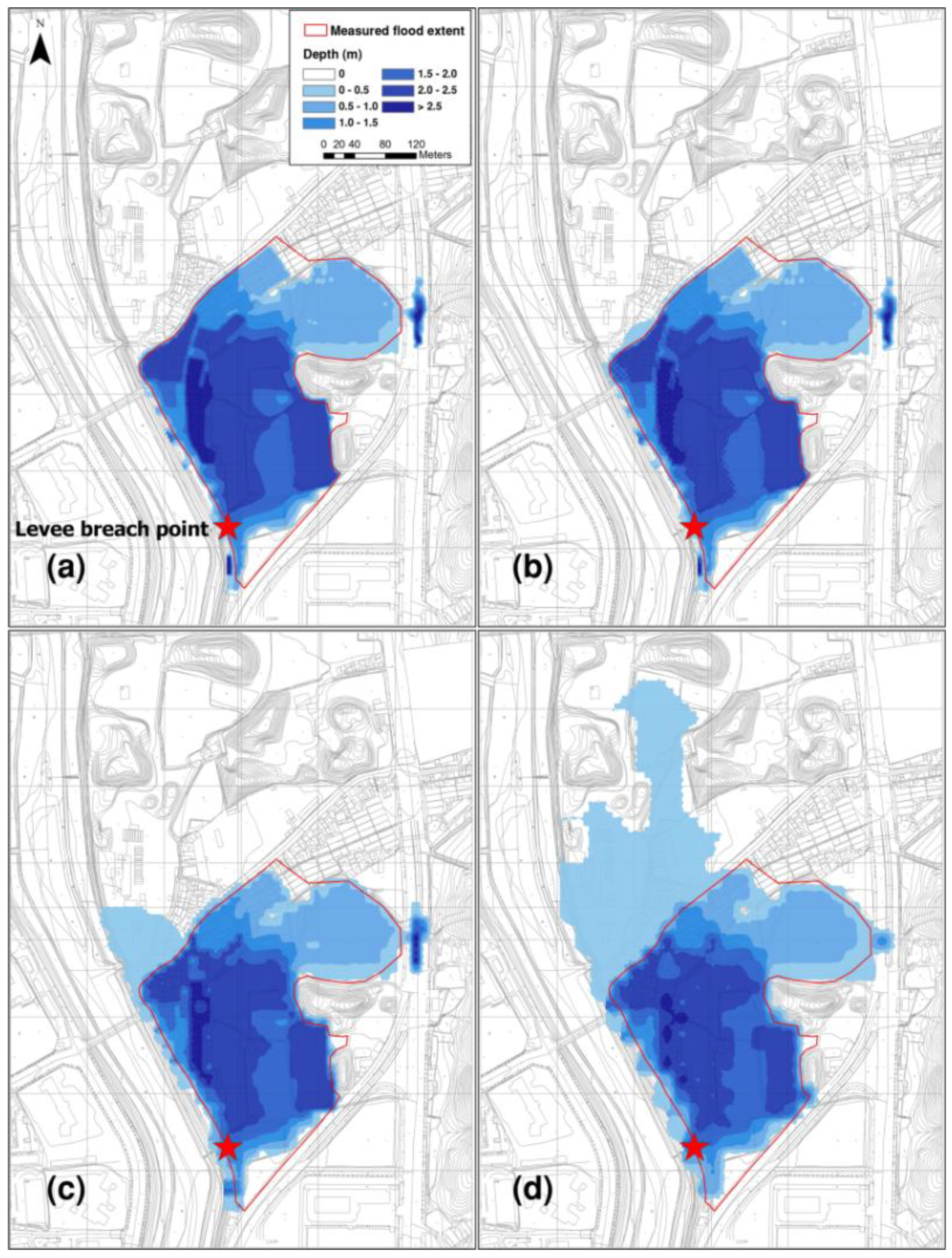
4.3. Real-Time Spatial Flood Inundation Analysis

4.3.1. Establishing Input Data

The 20-m wide left-hand side levee placed around 9 km downstream from Shingok GS (Figure 4) partially failed through a half hour duration of a J-11 event [41]. This levee breach led to flooding in part of the study area and Figure 9 presents the estimated levee breach discharge from 1-D river modeling with neuro-fuzzy model. The applicability of the 2-D flood inundation model linked to 1-D river modeling using the neuro-fuzzy model was tested in this area. That is, the estimated levee breach discharge (Figure 9) based on breach width and duration was applied to 2-D flood model as a boundary condition for flood inundation analysis in the study area.

Topographic data were provided as a digital contour map derived from a 1:1000-scale terrain map containing contour lines and spot heights (http://ngii.go.kr). Digital contour lines were subsequently converted to points and combined with spot heights to create a TIN (Triangulated Irregular Network). The structured grids with uniform resolution of 2, 4, 10, and 20 m were created with ArcGIS 10.0 (ESRI, Redlands, CA, USA) to examine the run-time and accuracy of 2-D flood model. Terrain elevations were extracted at grid nodes from TIN DTM (Digital Terrain Model).

4.3.2. Real-Time 2-D Inundation Analysis

The accuracy and computational efficiency including flood depth, goodness of fit, and run-time were estimated to examine the applicability of 2-D flood model for real-time inundation analysis. Grids with 2, 4, 10, and 20 m resolution were applied to the 2-D flood model and the comparison of observed and estimated flood extent due to levee breach are shown in Figure 10. The solid red line in Figure 10 presents the field surveyed flood extent by K-water (http://kwater.or.kr) and was supplied from Water Resources Management Information System (http://wamis.go.kr). The estimated flood area with grid size of 2 and 4 m was in agreement with the observed flood extent, whereas the estimated flood area with 20 m resolution grid was much wider than the observed one.

A fit ($F_A$) shown agreement between observed and estimated flood extent was computed using Equation (9) to quantitatively examine the model accuracy. The underestimation ($F_U$) and overestimation ($F_O$) were also computed using Equations (10) and (11), respectively.

$$F_A=\frac{A_e\cap A_o}{A_e\cup A_o}$$

(9)

$$F_O=\frac{A_o-A_e\cap A_o}{A_e\cup A_o}$$

(10)

$$F_U=\frac{A_e-A_e\cap A_o}{A_e\cup A_o}$$

(11)

where $A_e$ and $A_o$ are the estimated and observed flood extent area, respectively. The symbols $\cap$ and $\cup$ represent the intersection and union of two domains, respectively. The value of $F_A$ equals to 1 when two domains match perfectly, and 0 when no intersection area [42]. Wadey et al. [43] evaluated the fit ($F_A$) as three parts; good fit (>0.75), moderate fit (0.50~0.75), and poor fit (<0.50).

The computed maximum flood depth and the ratio of flood extent ($F_U$, $F_O$ and $F_A$) are presented in

Table 6. Maximum inundation depth and inundated area.

Grid Resolution (m)	Fit (%)			Flood Depth (m)		Flooded Area (km2)	Run Time (second)
	${\mathit{F}}_{\mathit{U}}$	${\mathit{F}}_{\mathit{O}}$	${\mathit{F}}_{\mathit{A}}$	Max.	Mean
2	6.45	6.32	87.23	3.17	2.97	2.97	76,365
4	6.05	7.66	86.29	3.09	2.89	2.89	15,707
10	5.10	16.86	78.03	2.89	2.68	2.68	195
20	2.97	39.72	57.31	2.81	2.51	2.51	21

. The maximum flood depth varied between 2.51 and 2.97 m and the agreement ($F_A$) varied between 0.57 and 0.87 depending on the grid size. That is, the difference of maximum flood depth varied from 8 (3%) to 36 cm (15%) and $F_A$ difference varied from 0.01 (1%) to 0.30 (34%) compared with the predictions of 2 m grid. The underestimation ($F_U$) decreased and the overestimation ($F_O$) was the reverse, as the grid size increased. In addition, the deep flood depth (>1.5 m) was spread widely across the entire flood extent regardless of grid size (Figure 10). This appears to be because of the topography of the region where the flooding took place. The area is a lower-land district than the nearby elevation, which served as a detention pond in the flooded area.

For real-time flood inundation analysis, the model run time is no less important than the model accuracy. Therefore, this study introduced the computational efficiency which is defined as model accuracy relative to computational effort in order to consider these two important factors. The run times of 2-D flooding model is measured to quantify computational effort. The model was executed using a 3.60 GHz Intel^® Core™ i7-4790 CPU with 32 GB RAM.

This study quantitatively examined the computational efficiency of 2-D flooding model by the grid size to find the optimal grid resolution for real-time inundation analysis. The computational efficiency of the grid resolution in the flooding model is revealed by plots of run times versus fit (${\mathrm{F}}_{\mathrm{A}}$) on semilog axis in Figure 11. Figure 11 represented that as the grid size increased, the model accuracy decreased slightly, while the run time diminished much more rapidly. When applying the high resolution (2 and 4 m) grids, the accuracy (${\mathrm{F}}_{\mathrm{A}}$) exceeded 85%, but it took a considerable run time (>15,707 s).

On the other hand, at the lowest grid resolution (20 m), the run time was the fastest (3 s) but the accuracy was the lowest (<57%). The accuracy was about 10% degraded and run time was almost two orders of magnitude faster in 10 m grid size than those of 4 m grid size. In the 20 m grid size, the accuracy was degraded by 27% and the model was executed just an order of magnitude faster compared with the 10 m grid size. The slope of the computational efficiency (fit vs. run time) of the model according to grid size shown in Figure 11 represented a significant change at the resolution of 10 m. This result indicates that 10 m grid resolution is a more realistic option with respect to real-time inundation analysis considering model run time and accuracy (78% and 192 s) with good fit condition (>75%) of Wadey et al. [43]. Although this simulation was performed on a home-use computer, if a high-performance computer or parallel computing including OpenMP (Open Multi-Processing) and MPI (Message Passing Interface) is used for flood inundation analysis, it is expected that more accurate results could be provided in real time.

5. Conclusions

In order to resolve the problems of the hydrological rainfall-runoff models that are currently applied for flood forecasting in South Korea, this study proposed a methodology for real-time flood forecasting and inundation analysis by developing an ANFIS that is easy to forecast with simple input variables and linking it with 1-D and 2-D hydrodynamic models.

The neuro-fuzzy flood forecasting model (ANFIS) developed was applied to the Jungrang Stream in South Korea. The combinations of various input variables including rainfall and water level were organized to find the optimal model for flood forecasting in the study area. The M-3 model (the combination of R(t), R(t-1), H(t), H(t-1), and H(t-2)) was chosen as the optimal combination of input variables based on the quantitative analysis of statistical indices by comparing observed and forecasted values. The parameters of the MF were determined in the processes of training and checking. The numbers of MFs and ANFIS model rules were determined by using the SC approach to shorten the execution time and optimize the input space partitioning. This study used the M-3 neuro-fuzzy model with two MFs and two rules for each input variable.

For the point flood forecasts, 13 rainfall events were applied to the testing process of ANFIS model and the performance of the model was evaluated using statistical indices (RMSE, NSEC, CC, and RPE) by comparing observations and forecasts for six lead times (0.5, 1.0, 1,5, 2.0, 2.5, and 3.0 h). The statistical indices indicated considerable accuracy up to 3.0 hour lead time, even if the accuracy decreased as the lead time increased. For the section flood forecasting, the discharge and water level forecasted by the ANFIS were applied to the 1-D hydrodynamic model (FLDWAV) as the upstream and downstream boundary conditions. The RMSEs between these two showed good agreement with 5.3, 16.1, and 21.5 cm for lead times of 1.0, 2.0, and 3.0 h, respectively. For the spatial inundation analysis, the levee breach discharge estimated from FLDWAV was applied as a boundary condition of 2-D inundation model for the study area where flooding occurred during J-11 event. This study examined the computational efficiency of the 2D flood model according to grid size to find the optimal grid resolution for real-time inundation analysis and demonstrated that the 10 m grid resolution was the most appropriate considering the model accuracy and execution time.

Flood forecasting using the neuro-fuzzy model developed in this study took less than 5 seconds because the output is immediately produced once the transmitted data are inputted. Also, under the condition that the input and topographic data, except for the boundary conditions, are established, 1-D river analysis was completed within 1 minute and 2-D inundation analysis took about 3 min. This demonstrated that the entire process of flood forecasting and inundation analysis was carried out within 5–10 min, enabling real-time flood forecasting. The methodology proposed in this study is expected to contribute to securing lead time for evacuating residents and protecting facilities at risk due to flooding.

References

1. Chang, F.J.; Chen, Y.C. A counterpropagation fuzzy-neural network modeling approach to real time streamflow prediction. J. Hydrol. 2001, 245, 153–164. [Google Scholar] [CrossRef]
2. Bazartseren, B.; Hildebrandt, G.; Holz, K.-P. Short-term water level prediction using neural networks and neuro-fuzzy approach. Neurocomputing 2003, 55, 439–450. [Google Scholar] [CrossRef]
3. Kraijenhoff, D.A.; Moll, J.R. River Flow Modeling and Forecasting; Springer: Berlin/Heidelberg, Germany, 2003. [Google Scholar]
4. Rodríguez-Iturbe, I.; Valdés, J.B. The geomorphologic structure of hydrologic response. Water Resour. Res. 1979, 15, 1409–1420. [Google Scholar] [CrossRef]
5. Ministry of Construction & Transportation (MCT). Improvement of Flood Forecasting Program for Major Streams; Ministry of Construction & Transportation: Seoul, Korea, 2005; pp. 1–195.
6. Nguyen, P.K.T.; Chua, L.H.C.; Son, L.H. Flood forecasting in large rivers with data-driven models. Nat. Hazards 2014, 71, 767–784. [Google Scholar] [CrossRef]
7. Khatibi, R.; Ghorbani, M.A.; Kashani, M.H.; Kisi, O. Comparison of three artificial intelligence techniques for discharge routing. J. Hydrol. 2011, 403, 201–212. [Google Scholar] [CrossRef]
8. Hsu, K.; Gupta, H.V.; Sorooshian, S. Artificial neural network modelling of the rainfall-runoff process. Water Resour. Res. 1995, 31, 2517–2530. [Google Scholar] [CrossRef]
9. Tokar, A.S.; Johnson, P.A. Rainfall-runoff modelling using artificial neural networks. J. Hydraul. Eng. 1999, 4, 232–239. [Google Scholar]
10. Sudheer, K.P.; Gosain, A.K.; Ramasastri, K.S. A data-driven algorithm for constructing artificial neural network rainfall-runoff models. Hydrol. Processes 2002, 16, 1325–1330. [Google Scholar] [CrossRef]
11. Jain, A.; Sudheer, K.P.; Srinivasulu, S. Identification of physical processes inherent in artificial neural network rainfall-runoff models. Hydrol. Processes 2004, 118, 571–581. [Google Scholar] [CrossRef]
12. Chang, T.K.; Talei, A.; Chua, L.H.C.; Alaghmand, S. The Impact of Training Data Sequence on the Performance of Neuro-Fuzzy Rainfall-Runoff Models with Online Learning. Water 2019, 11, 592. [Google Scholar] [CrossRef]
13. Taleia, A.; Chua, L.H.C.; Wong, T.S.W. Evaluation of rainfall and discharge inputs used by Adaptive Network-based Fuzzy Inference Systems (ANFIS) in rainfall-runoff modeling. J. Hydrol. 2010, 391, 248–262. [Google Scholar] [CrossRef]
14. Hosseinia, S.M.; Mahjouri, N. Integrating Support Vector Regression and a geomorphologic Artificial Neural Network for daily rainfall-runoff modeling. Appl. Soft Comput. 2016, 38, 329–345. [Google Scholar] [CrossRef]
15. Komasi, M.; Sharghi, S. Hybrid wavelet-support vector machine approach for modelling rainfall–runoff process. Water Sci. Technol. 2016, 73, 1937–1953. [Google Scholar] [CrossRef]
16. Bartolettia, N.; Casaglia, F.; Marsili-Libellib, S.; Nardia, A.; Palandri, L. Data-driven rainfall/runoff modelling based on a neuro-fuzzy inference system. Environ. Modell. Softw. 2018, 106, 35–47. [Google Scholar] [CrossRef]
17. Imrie, C.E.; Durucan, S.; Korre, A. River flow prediction using artificial neural networks: Generalisation beyond the calibration range. J. Hydrol. 2000, 233, 138–153. [Google Scholar] [CrossRef]
18. Hu, T.S.; Lam, K.C.; Ng, S.T. River flow time series prediction with a range-dependent neural network. J. Hydrol. Sci. 2001, 46, 729–745. [Google Scholar] [CrossRef]
19. Kumar, D.N.; Raju, K.S.; Sathish, T. River flow forecasting using recurrent neural networks. Water Resour. Manag. 2004, 18, 143–161. [Google Scholar] [CrossRef]
20. Yarar, M.; Onucyildiz, M.; Copty, N.K. Modelling level change in lakes using neuro fuzzy and artificial neural networks. J. Hydrol. 2009, 365, 329–334. [Google Scholar] [CrossRef]
21. He, Z.; Wen, X.; Liu, H. A comparative study of artificial neural network, adaptive neuro fuzzy inference system and support vector machine for forecasting river flow in the semiarid mountain region. J. Hydrol. 2014, 509, 379–386. [Google Scholar] [CrossRef]
22. Nguyen, P.K.T.; Chua, L.H.C.; Talei, A.; Chai, Q.H. Water level forecasting using neuro-fuzzy models with local learning. Neural Comput. Appl. 2018, 30, 1877–1887. [Google Scholar] [CrossRef]
23. Zhang, Z.; Zhang, Q.; Singh, V.P.; Shi, P. River flow modelling: Comparison of performance and evaluation of uncertainty using data-driven models and conceptual hydrological model. Stoch. Environ. Res. Risk Assess. 2018, 32, 2667–2682. [Google Scholar] [CrossRef]
24. Luk, K.C.; Ball, J.E.; Sharma, A. An application of artificial neural networks for rainfall forecasting. Math. Comput. Model. 2001, 33, 683–693. [Google Scholar] [CrossRef]
25. Ramirez, M.C.P.; Velho, H.F.C.; Ferreira, N.J. Artificial neural network technique for rainfall forecasting applied to the Sao Paulo region. J. Hydrol. 2005, 301, 146–162. [Google Scholar] [CrossRef]
26. Mekanik, F.; Imteaz, M.A.; Talei, A. Seasonal rainfall forecasting by adaptive network-based fuzzy inference system (ANFIS) using large scale climate signal. Clim. Dyn. 2016, 46, 3097–3111. [Google Scholar] [CrossRef]
27. Pham, Q.B.; Yang, T.-C.; Kuo, C.-M.; Tseng, H.-W.; Yu, P.-S. Combing Random Forest and Least Square Support Vector Regression for Improving Extreme Rainfall Downscaling. Water 2019, 11, 451. [Google Scholar] [CrossRef]
28. Han, Y.; Zou, Z.; Wang, H. Adaptive neuro fuzzy inference system for classification of water quality status. J. Environ. Sci. 2010, 22, 1891–1896. [Google Scholar] [CrossRef]
29. Khaki, M.; Yusoff, I.; Islami, N. Application of the Artificial Neural Network and Neuro-fuzzy System for Assessment of Groundwater Quality. Clean-Soil Air Water 2015, 43, 551–560. [Google Scholar] [CrossRef]
30. Yaseen, Z.M.; Ramal, M.M.; Diop, L.; Othman Jaafar, O.; Demir, V.; Kisi, O. Hybrid Adaptive Neuro-Fuzzy Models for Water Quality Index Estimation. Water Resour. Manag. 2018, 32, 2227–2245. [Google Scholar] [CrossRef]
31. Jang, J.S. ANFIS: Adaptive-network-based fuzzy inference system. IEEE Trans. Syst. Man Cybern. 1993, 23, 665–685. [Google Scholar] [CrossRef]
32. Takagi, T.; Sugeno, M. Fuzzy identification of systems and its applications to modeling and control. IEEE Trans. Syst. Man Cybern. 1985, 15, 387–403. [Google Scholar] [CrossRef]
33. Al-Hmouz, A.; Shen, J.; Al-Hmouz, R. Modeling and simulation of an adaptive neuro-fuzzy inference system (ANFIS) for mobile learning. IEEE Trans. Learn. Technol. 2012, 5, 226–237. [Google Scholar] [CrossRef]
34. Jang, J.S.R.; Sun, C.T.; Mizutani, E. Neuro-Fuzzy and Soft Computing: A Computational Approach to Learning and Machine Intelligence; Prentice Hall: Upper Saddle River, NJ, USA, 1997. [Google Scholar]
35. Fread, D.L.; Lewis, J.M. NWS FLDWAV Model; Hydrologic Research Laboratory Office of Hydrology, National Weather Service; NOAA: Silver Spring, MD, USA, 1998. [Google Scholar]
36. Chow, V.T.; Maidment, D.R.; Mays, L.W. Applied Hydrology; McGRAW-HILL International Editions: New York, NY, USA, 1988. [Google Scholar]
37. Kim, B.; Kim, T.H.; Kim, J.H.; Han, K.Y. A well-balanced unsplit finite volume model with geometric flexibility. J. Vibioeng. 2014, 16, 1574–1589. [Google Scholar]
38. Son, A.L.; Kim, B.; Han, K.Y. A simple and robust method for simultaneous consideration of overland and underground space in urban flood modeling. Water 2016, 8, 494. [Google Scholar] [CrossRef]
39. Kim, T.H.; Kim, B.; Han, K.Y. Application of Fuzzy TOPSIS to Flood Hazard Mapping for Levee Failure. Water 2019, 11, 592. [Google Scholar] [CrossRef]
40. Kar, A.K.; Goel, N.K.; Lohani, A.K.; Roy, G.P. Application of clustering techniques using prioritized variables in regional flood frequency analysis—Case study of Mahanadi Basin. J. Hydrol. Eng. 2012, 317, 213–223. [Google Scholar] [CrossRef]
41. K-Water. (Flood Map Fundamental Investigation) Flood Inundation History Report; K-Water: Daejeon, Korea, 2005; pp. 1–83. [Google Scholar]
42. Bates, P.D.; Dawson, R.J.; Hall, J.W.; Horritt, M.S.; Nicholls, R.J.; Wicks, J.; Hassan, M.A.A.M. Simplified two-dimensional numerical modelling of coastal flooding and example applications. Coast. Eng. 2005, 52, 793–810. [Google Scholar] [CrossRef]
43. Wadey, M.P.; Nicholls, R.J.; Hutton, C. Coastal flooding in the Solent: An integrated analysis of defences and inundation. Water 2012, 4, 430–459. [Google Scholar] [CrossRef]
Figure 1. Flow chart of this study.
Water 11 00919 g001
Figure 2. First-order Takagi–Sugeno inference scheme [31].
Water 11 00919 g002
Figure 3. Structure of the adaptive neuro-fuzzy inference system (ANFIS) [31].
Water 11 00919 g003
Figure 4. Study area and gauge stations.
Water 11 00919 g004
Figure 5. Structure of the ANFIS model in this study.
Water 11 00919 g005
Figure 6. Comparison of observation and forecasted water-level at Jungrang GS for J-11 event.
Water 11 00919 g006
Figure 7. Comparison of observed and converted discharge for J-11 event at Shingok GS.
Water 11 00919 g007
Figure 8. Comparison of predicted water level using observed and forecasted boundary conditions at a distance of 6 km downstream from Jungrang GS for each lead time (J-11 event).
Water 11 00919 g008aWater 11 00919 g008b
Figure 9. Estimated levee breach discharge.
Water 11 00919 g009
Figure 10. Comparison of observed and estimated flood extent by grid size: (a) 2, (b) 4, (c) 10, and (d) 20 m.
Water 11 00919 g010
Figure 11. Computational efficiency according to the grid resolution.
Water 11 00919 g011