Abstract
Soil moisture (SM) is an important variable for the terrestrial surface system, as its changes greatly affect the global water and energy cycle. The description and understanding of spatiotemporal changes in global soil moisture require long time-series observation. Taking advantage of the European Space Agency (ESA) Climate Change Initiative (CCI) combined SM dataset, this study aims at identifying the non-linear trends of global SM dynamics and their variations at multiple time scales. The distribution of global surface SM changes in 1979–2016 was identified by a non-linear methodology based on a stepwise regression at the annual and seasonal scales. On the annual scale, significant changes have taken place in about one third of the lands, in which nonlinear trends account for 48.13%. At the seasonal scale, the phenomenon that “wet season get wetter, and dry season get dryer” is found this study via hemispherical SM trend analysis at seasonal scale. And, the changes in seasonal SM are more pronounced (change rate at seasonal scales is about 5 times higher than that at annual scale) and the areas seeing significant changes cover a larger surface. Seasonal SM fluctuations distributed in southwestern China, central North America and southern Africa, are concealed at the annual scale. Overall, non-linear trend analysis at multiple time scale has revealed more complex dynamics for these long time series of SM.
1. Introduction
Soil moisture (SM), as an important element of the land surface system, playing an indispensable role in ecology, agriculture, as well as hydrological and surface modeling research [1]. It stores precipitation, provides essential water for plants, thus affecting ecosystem development, and participates in the global water cycle and energy balance through evapotranspiration. In past decades, changing climate factors such as precipitation and evapotranspiration associated with global warming and greening have affected global soil water content. The extent which global SM has changed is a paramount issue pertaining to climate change and its variability, due to the importance and heterogeneity of these variations [2]. In view of this problem, some research has been conducted. On a global scale, Dorigo et al. [3] assessed the trend distributions for the 1988–2010 period. Feng and Zhang [4] studied the global trends in SM to test the paradigm of a “dry [region] gets drier, wet gets wetter”. Similar trend analyses have been performed on regional scales as well [5,6,7,8,9,10]. In all the aforementioned studies, SM is assumed to change linearly, although some of the changes occurring in long time series could be non-linear. The disadvantage of simple linear analysis is that the overall trend of SM during long time may conceal the actual change and change rate in different periods, thus interfering with the relevant analysis of SM-climate change feedback mechanism, water cycle, water resources utilization and so on. In contrast, non-linear analysis can reveal the transition of variation during long periods which is closer to the real change of factors. For example, Pan et al. [11] revealed the existence of concealed browning trends of vegetation, when the vegetation of some regions turns brown or sees a slowdown in greening, in spite of an overall tendency for global vegetation greening. Thus, the subject of hidden trends in SM merits further study.
In addition to a non-homogeneous spatial distribution, SM has been shown to be heterogeneous at different time scales by a large number of studies [12,13,14,15,16,17]. The spatial distribution of the 38-year average SM at the seasonal scales is significantly different with that at the annual scales, owing to the dominance of climate-related seasonal SM variations which are closely related to phenology and vegetation growth. It is therefore necessary to analyze the multi-year dynamical changes of SM at both the annual and seasonal time scales. Dorigo et al. [3] have shown global trend patterns at the annual and the seasonal time scales, respectively. However, difference and connection between the results at two time scales have not yet been pointed out. It can be found that global trend patterns at the annual and the seasonal time scales in that study were differing, i.e., that in some areas, inter-annual changes occurring during a given season were not consistent with changes happening during other seasons or at the annual scale. Such a phenomenon was also documented in some studies of regional SM dynamics in China, e.g., Qiu et al. [18] and Chen et al. [19]. The differences between the dynamic trends of SM at various time scales have yet to be examined.
For a large-scale SM study, remote-sensing SM data present the advantages of periodicity, long time series, wide spatial range and real-time observation, all of which are conducive to the analysis of spatial distribution and temporal trends of changes. Whereas traditional SM measurement methods such as drying and time domain reflectance are time-consuming, laborious and space-constrained [20,21], and model simulation data have strong correlation both on spatial and temporal dimensions, remote-sensing data provides a strong support for global SM research [22,23], although it’s observations are confined to the surface. Many studies have demonstrated the feasibility of remote-sensing SM techniques for climate change, land-atmosphere interaction [24,25,26], ecology [27,28], hydrology [29,30,31] and drought [32,33,34] research studies.
As a result, two main purposes encourage us to investigate global SM dynamics from new perspectives based on a remote-sensing SM product. Firstly, although linear trends of global SM have been presented before, it is still necessary to study the dynamics of SM change over longer periods using a non-linear method, because non-linear trends have been illustrated to show concealed changes, such as the vegetation trend discussed above. Secondly, there are climate-related fluctuations in SM content during the seasons whereby, generally, it is wetter in summer and drier in winter. Whether seasonal SM has changed under the long-term climate change remains to be clarified. Quantifying seasonal SM changes may shed new light on interaction between the ground surface SM and climate change and its impacts on the hydrological cycle. In this study, we reveal non-linear trends of global surface SM and quantify seasonal SM changes and the difference between annual and seasonal SM dynamics using the stepwise regression method and trend consistency analysis with the aim of further understanding global surface SM changes and the impact of precipitation.
This paper is organized as follows. Firstly, based on gridded remote-sensing data, area-averaged surface SM at hemisphere scale were calculated to analyze the distribution of monthly SM content and annual and seasonal variation of hemisphere SM. Then, non-linear trend analysis of global surface SM at each pixel will be performed at both the annual and seasonal scales. In addition to the spatial trend distributions, the time-varying rates of SM were calculated at different time scales to explore the difference between multi-scale SM trends. The datasets and methodology are described in Section 2. Section 3 delineates the results of the study, including the area-averaged surface SM trend, the SM trend distributions and their time-varying rates at the annual and the seasonal scales. At last, the comparison between the surface SM trends obtained with the remote sensing SM dataset and those derived from reanalysis product, as well as the trends of precipitation were estimated to test the reliability of results and explore the relationship between surface SM and precipitation change. The evaluation of the results, as well as comparisons between the results of this study and previous research, and the influence of precipitation on surface SM, are discussed in Section 4.
2. Data and Methods
2.1. Data
The Climate Change Initiative (CCI) dataset of the European Space Agency (ESA) is adopted for monitoring the global SM trend and was obtained from the ESA website. To alleviate the effect of the uneven time series of the various SM datasets (due to the difference in satellite service time), the ESA CCI SM dataset has combined active and passive SM products derived from microwave remote-sensing measurements. This ESA CCI SM v4.2 dataset provides the longest time series to date, covering the period 1979–2016, and has been widely used for various Earth system research [35]. The dataset depth is 10 cm and accuracy is deemed acceptable, with validation by global ground-based observations yielding a mean correlation coefficient (R) and root mean square error (RMSE) of 0.46 and 0.04 cm3/cm3, respectively. In order to evaluate the results based on the ESA CCI SM dataset, European Centre for Medium-Range Weather Forecasts (ECMWF) Interim Reanalysis (ERA-Interim) monthly average SM data were also analyzed for comparing which provide a reanalysis of the global atmosphere covering the data-rich period starting from 1979, and continuing to the present time. The data assimilation system used to produce ERA-Interim is based on a 2006 release of the Integrated Forecast System (IFS). This product includes four volumetric soil water layers with depths of 7 cm, 28 cm, 100 cm and 255 cm, respectively. In order to be comparable with the ESA CCI SM product, only the data of the soil water layer 1 (0–7 cm) estimated from 1979 to 2016 and with a spatial resolution of 0.25° × 0.25°, were used in the study.
The Multi-Source Weighted-Ensemble Precipitation (MSWEP) product is a global grid precipitation (P) dataset specifically designed for hydrological modeling. This dataset is unique in that it optimally merges a wide range of data sources based on gauges (GPCC, CPC Unified, and CHPclim), remote sensing (CMORPH, GSMaP-MVK, and TMPA 3B42RT), and weather models (ERA-Interim, JRA-55, and NCEP-CFSR) to provide the best possible P estimates at a global scale. This dataset presents the advantages of a long time scale and a high spatial resolution. The data was resampled from 0.1° to 0.25° spatial resolution via the nearest neighbor method for the 1979–2016 period so that it can be compared with the SM datasets.
2.2. Methodology
2.2.1. Trend Analysis
As shown in Figure 1, the area-averaged SM trends and trend distributions obtained from the ESA CCI SM data were analyzed both at the annual and seasonal time scales. Here, the seasons are defined as follows: the first season is from December to next February, the second season from March to May, the third season from June to August, and the fourth season from September to November. SM data at the annual and seasonal scales were both generated from monthly grid SM data, which were obtained by averaging the valid daily SM data pixel by pixel. For area-averaged SM, annual trends and seasonal inter-annual trends were estimated via polynomial fitting of the relationship between the years and the annual/seasonal hemispherical mean SM value. For determining the distribution of global trends, the non-linear methodology was carried out pixel-by-pixel on the annual/seasonal grid SM data to discover the location of each trend type. Based on the trend recognition results, some comparisons are carried out between results at the annual and seasonal scales based on statistical analysis, including trend distribution, change rates, area, and meridional distribution of trend, to reveal the differences in trend caused by the various time scales.
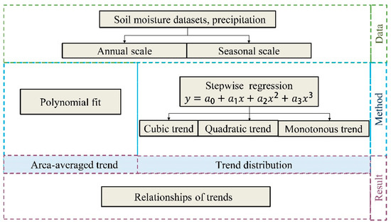
Figure 1.
Brief flow scheme of trend analysis.
Additionally, trend distributions of precipitation were estimated via the nonlinear methodology. After resampling these data to an interval similar to that of the SM dataset, consistency between the distributions of the precipitation trends and the ESA CCI SM trend distribution was calculated to estimate the effects of these two climate factors on SM changes. Meanwhile, to verify the validity of the ESA CCI SM data trends, the ERA-Interim reanalysis SM data were analyzed by the same methodology. This allows the differences and the consistency between these two SM trend distributions to be estimated. Based on the trends classification, consistent areas were classified as fully consistent and currently consistent areas. For example, cubic up-down-up trends are currently consistent with quadratic down-up trends and linear up trends.
2.2.2. Trend Recognition
In this study, a non-linear methodology was employed to estimate trends of variables whereby variations were divided into cubic, quadratic, monotonic, and insignificant trends. First, stepwise regression, which has been proved to be effective in revealing variable trends, was used on the variables time series, based on the following equation [36]:
where x is the year order, y is the variable such as annual SM, and a0, a1, a2, a3 are coefficients. In stepwise regression, predictive variables are chosen automatically to achieve least predictive variables while ensuring optimal predictive ability.
The resulting model was tested by F-test for both the regression model and all its coefficients so that the trend type of variable was determined by the highest order of x. When the coefficient a3 passes the significance test, the trend is cubic; in the case when the a2 coefficient passes while a3 does not pass the significance test, the trend is quadratic temporarily. Other results are regarded as monotonic trends, which are separated into significant and insignificant trends by a significance test. As shown in Figure 2, after stepwise regression with the F-test and the coefficient test, the trend was recognized by diagnosing the effectiveness of the turning points which were extreme points of regression model. For a regression model, if two turning points distributed in the effective region of years (0~maximum year order) exist, it is regarded as a cubic trend model; if only one turning point belongs to the effective region, it is a quadratic trend model; and if no turning point exists in the time series, the model is regarded as linear. The specific trend is then determined according to the sign of the effective coefficient. After determining the trend type, the data of each stage were linearly regressed to estimate the change rate of soil moisture at each stage, taking the turning point as the time boundary.
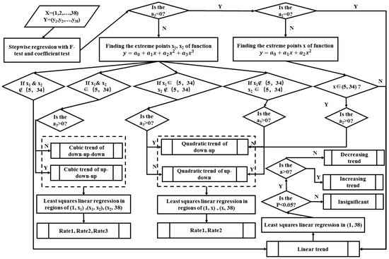
Figure 2.
Flow chart of trend recognition.
For nonlinear trends, the last trend (the part of the trend which follows the last turning point) is regarded as the current trend of SM change, and can be classified as positive or negative. If the current trend is increasing, such as the up-down-up and down-up trend, it is recognized as a positive trend; by contrast, a down-up-down or up-down trend is regarded as negative. Similarly, for the linear case, increasing (decreasing) trend is recognized to be positive (negative). Finally, trends were further divided into the seven following types: two cubic trends (up-down-up, and down-up-down), two quadratic trends (down-up, and up-down), two linear trends (up, and down), and insignificant trend. The rates of change for each period of non-linear and linear trends were estimated by ordinary least squares linear regression.
3. Results
3.1. Area-Averaged Soil Moisture (SM)
Monthly SM data constitute the basis of SM trend analysis at the annual and seasonal scales. As shown in Figure 3a, hemispherical monthly mean SM content ranges from 0.05 m3/m3 to 0.25 m3/m3 and average SM in the northern hemisphere is lower than that in the southern hemisphere (0.13 m3/m3 to 0.24 m3/m3). The distribution peaks in July (February) in the northern (southern) hemisphere respectively which means that SM is highest in summer. The global spatial pattern of mean SM content from 1979 to 2016 (Figure 3b) exhibit large variations, with values ranging from 0 to 0.41 m3/m3. The SM content in southern China and central South America is the highest, while that in the Sahara Desert and the Arabian Peninsula is the lowest. SM values in regions of tropical forests i.e., the Amazon Plain, Congo basin and Indonesia are set to NaN in original datasets because dense vegetation in such areas limits the accuracy of SM retrieval from microwave sensors.
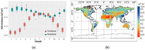
Figure 3.
(a) Statistics of global average soil moisture (SM) at monthly scale in 1979–2016; (b) global pattern of SM average over the 1979–2016 period.
Figure 4 displays the annual and seasonal values of hemispherical mean SM for the entire period of the dataset and their corresponding trends. The present mean SM over the northern hemisphere is about 0.02 m3/m3 higher than that of the 1980s at both the annual and all the seasonal scales. The maximum seasonal mean SM is reached in summer (values mostly in the 0.16~0.18 m3/m3 range); followed by autumn (0.12~0.14 m3/m3), spring (0.08~0.12 m3/m3), and winter (0.05~0.09 m3/m3) in the northern hemisphere.
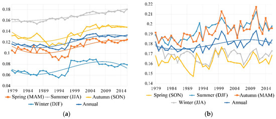
Figure 4.
Annual and seasonal mean SM in the northern hemisphere (a) and in the southern hemisphere (b) and their trends between 1979 and 2016.
In the northern hemisphere, the trend of mean SM at the annual scale between 1979 and 2016 (dark blue line in Figure 4) follows a cubic down-up-down pattern. The annual values indeed show a gradual SM decrease from 1979 to the mid-1990s, followed by a period of increase (mid-1990s to late 2000s) and a more stable period starting 2010. Similar to the annual trend, the hemispherical mean SM trends in spring, autumn and winter are of the cubic down-up-down type, whereas that in summer is a monotonously increasing trend. This implies that wetter seasons get wetter, while dryer seasons get slightly dryer in recent years in the northern hemisphere.
In the southern hemisphere, mean SM fluctuates greatly at both seasonal and annual scales and polynomial regression relationship with years is weak. Mean SM in summer and autumn (0.18~0.22 m3/m3) has increased during the period of 1979–2016 which is higher than that in spring and winter (0.15~0.18 m3/m3). This means that phenomenon of “wetter seasons are wetting” also exists in the southern hemisphere whereas there is no obvious increasing or decreasing trend SM in a dryer season.
3.2. Annual Trend Distribution
Through trend recognition, 32% of the total land pixels with valid SM time series are estimated to present a significant trend. According to the pie chart of trends in Figure 5, cubic trends (green and yellow in Figure 5) only account for 4.38% of the significant trends, are dispersed randomly within the areas of significant changes areas, and can therefore be considered negligible. Quadratic and linear trends account for 43.75% and 51.87%, respectively, which means that nonlinear and linear trends respectively account for half of all the significantly changed areas. Positive linear trends (dark blue in Figure 5) are distributed over the northeastern part of North America, the Sahara Desert in Africa, and the southern Arabian Peninsula. Within Asia, the areas are scattered throughout the continent from the northern West Siberian Plain in the north to the Irrawaddy River Basin (Myanmar) in the southeast. The distribution of the decreasing linear trend areas (red in Figure 5) is more widely distributed throughout the world, with various parts of the five inhabited continents being covered by this trend. Notable regions include the Cordillera in South America, the north and northeastern parts of Canada in North America, Ethiopia and Somalia in East Africa, Scandinavia in Europe, and the Japanese islands and Mekong river basin in Asia.
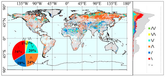
Figure 5.
Spatial distribution of the seven different trends of annual SM on all valid lands and its statistical pie chart and Meridional statistical distribution. Symbols in the legend “/\/”, “\/\”, “\/”, “/\”, “/”, “\”and “-” indicate “up-down-up,” “down-up-down,” “down-up,” “up-down,” “up,” “down” and “insignificant” trend, respectively.
The distribution of quadratic trends is as follows: the areas of “down-up” trend (light blue in Figure 5) are also largely represented in the results, being distributed within continental areas of northern Africa, central and east Asia, Central America, east Europe, and the western coast of central South America. The “up-down” trend (orange color in Figure 5) is similar to, but narrower than that of the linear ‘down’ trend. In the time series at each of these locations, the turning points (marking the year when the direction of the trends change) are not concentrated geographically (not shown). This means that the changes from up to down are slow rather than sudden.
From the distribution map, pixels belonging to the same trends are generally seen to be clustered together, except in the region of the Tibetan Plateau where negative trend areas are surrounded by regions of positive trends. The meridional distribution of the trends (Figure 5) highlights that the significant trends are mostly distributed within the northern hemisphere which is consistent with the result of area-averaged analysis. In particular, linear increasing trends mainly cover the mid and low latitude regions, while negative trends generally distribute towards higher latitudes. In addition, most of the positive trends are located in arid areas, including some areas where they have turned from drying to wetting such as part of northwest China. Through the regional statistic on continental scale (Table 1), regional proportions of significant changed area in Asia is the largest in six continents, which means that the SM content in Asia is more unstable than that in other regions. In addition, most of the regions with significant changes in Asia are inland areas, which are more likely to be affected by changes in surface cover types. Among the significant trends, a linear decreasing trend accounts for the largest proportion in North and South America, Asia and Europe, followed by a quadratic “up-down” trend, which means that majority of the significant change areas in these four continents are drying up. On the contrary, in Africa and Oceania, linear increasing trend and quadratic “down-up” trend account for more percentage, means that most of the significant change areas are getting wet.

Table 1.
Statistic of significant change in each continent.
Figure 6 shows the rates of change at each pixel before (Figure 6a) and after (Figure 6b) the turning point of the quadratic trends, calculated by linear regression. These rates mostly range between 0.6‰ and −0.6‰ m3/m3 per year which count for about 80% of all valid area (Figure 6c). Increasing rates of SM at the Turan Lowland, Kazakh Hills, Tibetan Plateau and Mekong River Basin in Asia are significantly higher than in other regions. Comparatively, SM content in northern and eastern Asia, the Brazilian Plateau, the Mississippi River Basin and southern Africa has been decreasing rapidly. Rates in mostly areas have no significantly change during period of 1979–2016 except a few regions (black ellipses in Figure 6). The SM in northern Canada, northern Russia, the Sahara Desert, the Mongolian Plateau and parts of the Loess Plateau (China) has changed from decreasing (rate ≥ 1‰ per year) to increasing (rate ≤ 1‰ per year). In the Tibetan Plateau, where SM increased significantly during the first period, a decreasing trend is seen in the later period. Although the SM rates of change in most regions of the world is stable, the regions seeing large changes, such as the Tibetan Plateau in China, require more attention and management measures to mitigate these changes.
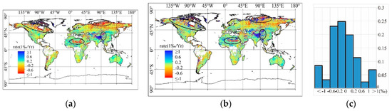
Figure 6.
Average rates of change of the annual SM trend before (a) and after (b) the turning point of the quadratic trends. (c) Statistics of global surface SM changing rates. Regions where the rate has changed significantly between the two periods are underlined by black ellipses.
3.3. Seasonal Trend Distributions
Figure 7 presents the trend distributions during the four seasons and their meridional distribution. In addition, the respective percentage of each trend is indicated in a separate panel (Figure 7e). These statistics vary largely depending on the season as shown in Table 2, and the percentage of areas with significant changes is 33%, 42%, 47%, and 38% from the first to the fourth season, respectively. This is larger than for the annual trends (32%). At every season, the number of pixels with linear trends is larger than that of non-linear trends, and the monotonously increasing trend (“up”) is the dominant trend, whereas the cubic seasonal trends are negligible. In the northern hemisphere, the meridional distribution of positive trends (quadratic ‘down-up’ trend and linear increasing trend) in four seasons is homogeneous, whereas the negative trends (quadratic ‘up-down’ trend and linear decreasing trend) present greatly seasonal variation. Variation of SM seasonal trend distributions did not show obvious regularity due to large land area and complex topography in the northern hemisphere. In the southern hemisphere, the dominant trend in summer (first season) and winter (third season) is positive trend and negative trend, respectively, which is consistent with the phenomenon of “wetter seasons get wetter, while dryer seasons get drier”.
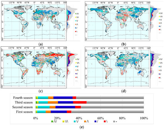
Figure 7.
Spatial distribution of the different trends of SM on all valid lands and their meridional distribution during the: (a) first season (winter in northern hemisphere while summer in southern hemisphere), (b) second season (spring in northern hemisphere while autumn in southern hemisphere), (c) third season (summer in northern hemisphere while winter in southern hemisphere), and (d) fourth season (autumn in northern hemisphere while spring in southern hemisphere). (e) Percentage of the respective trends at each season. Symbols in panels (a–d) are identical to those of Figure 5.
Table 2.
Pixel numbers of different trend at annual and seasonal scales and the percent account of all valid land pixels.
Spatial distribution of quarterly trends varies greatly such that most regions present different trends at the various seasons, or trends at the annual scale different from those at the seasonal scale. For example, the SM in the Tibetan Plateau and in northern Asia presents no significant trend during the first season, whereas significant trends can be seen both at the annual scale and during the other seasons. In northwestern Eurasia, central North America, central Africa, and the Brazil Plateau, the increasing current trend in the first season is different from the annual and other seasonal trends. In southeastern China, the SM is decreasing during the first and fourth seasons, but increasing in the second and third seasons, which explains why no significant change is observed at the annual scale.
Two main pieces of information arise from the comparison between the annual and the seasonal trends. First, the absence of change at the annual scale in some areas does not necessarily mean that no change occurred in these regions, e.g., southeastern China. This explains why the surface with significant seasonal changes is larger than that of annual changes. Second, the areas seeing significant changes at the annual scale do not always experience consistent changes depending on the season. Thus, in several instances, the annual variations misrepresent the actual changes of seasonal SM which are directly related to vegetation growth.
Besides, the changing rate of SM trends also differs depending on the scale (annual or seasonal). The seasonal variations of SM are more severe than the annual variations, with the seasonal changing rate of (ranging from −0.005 m3/m3 to 0.005 m3/m3 per year) being largely higher than that of the annual trends (between −0.001 m3/m3 and 0.001 m3/m3 per year). Most of the non-linear change rates have little difference between before and after the turning point, except for the areas underlined by black ellipses in Figure 8 where absolute value of change rate exceeds 0.005 m3/m3 per year. In the northern hemisphere, the rate of SM changes at higher latitudes largely differs with the season. During the first and the fourth season (winter and autumn), SM change rate in southwestern China, the Sahara, northern North America and northwestern Eurasia has increased, with the rate changing from decreasing to increasing in most of these regions. In summer, SM change rate in the region of the Tibetan Plateau has seen significant changes, with decreasing rates appearing in this area after the turning point and values exceeding 0.005 m3/m3 per year. In the southern hemisphere, in the Brazil Plateau and the southern part of central Africa, the increasing (decreasing) rates in summer (autumn and winter) slow down significantly during the second period (after the turning point). This implies that, in the northern hemisphere, the seasonal SM distribution and its change rate vary greatly with the seasons, while the change of seasonal SM in the southern hemisphere has slowed down and the seasonal difference is decreasing.
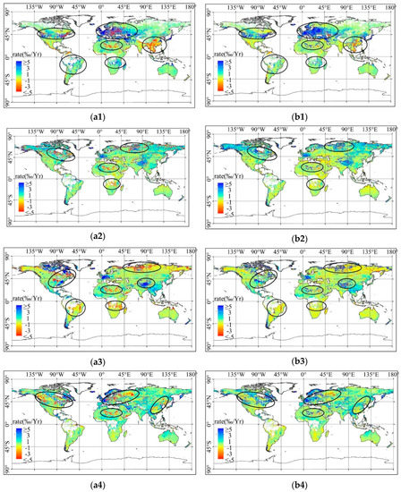
Figure 8.
Same as Figure 6, but for the seasonal rates of change. Prefix (a) and (b) indicate the rates before and after the turning points, respectively; and numbers 1 to 4 stand for the first to the fourth season, respectively.
4. Discussion
4.1. Evaluation of Results
To verify the results based on the ESA CCI SM dataset, the ERA-Interim reanalysis SM dataset has been analyzed via same methodology. Comparing the global maps of mean SM from 1979–2016, the map generated from the ESA CCI SM dataset (Figure 3b) is more detailed than that obtained from the ERA-Interim SM dataset (Figure 9a). This is due to the data at each pixel observed by remote sensing being independent from each other, in contrast with the re-analysis data which have a strong spatial correlation. Figure 9b,c show the trend patterns of the ERA-Interim SM, and its consistency with ESA CCI SM at the annual scale, respectively. The areas seeing significant trends are more extensive in the ERA-Interim SM than that in the ESA CCI SM. Regions with “up-down” trends in the Americas, parts of northern and western Asia, and northeastern Africa, are found to be consistent with the negative trends of the ESA CCI SM dataset. The largest wetting trends observed in the Turan Lowland (Russia), Irrawaddy River basin (Myanmar) and Loess Plateau (China) are also seen in the ERA-Interim SM dataset. Dramatic changes in high latitude and the Tibetan Plateau are not presented in results based on ERA-Interim SM dataset. Thus, the trends pattern of the ESA CCI SM dataset is mostly consistent with those obtained from the ERA-Interim reanalysis dataset, albeit with some differences in their spatial extent.
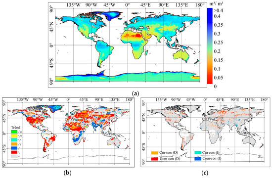
Figure 9.
(a) Global pattern of mean SM from 1979–2016 based on the ERA-Interim (European Centre for Medium-Range Weather Forecasts (ECMWF) Interim Reanalysis) SM dataset. (b) Spatial distribution of annual trends (b) from the ERA-Interim SM, and (c) their consistency with European Space Agency (ESA) Climate Change Initiative (CCI) SM. “Cur-con”, “Com-con”, “D”, and “I” are abbreviations for “Currently consistent”, “Completely consistent”, “decreasing”, and “increasing”, respectively.
However, there are some issues about the trend analysis results that should be discussed based on a quality assessment of the data. Firstly, the area-average SM in the mid-1990s is generally lower than that in other years due to missed daily SM data in the northern hemisphere which are largely related to coverage of data source sensors (AMI-WS (Active Microwave Instrument—Windscat) and SSMI (Special Sensor Microwave Imager) were used in 1990s). Although interpolated data via the PCHIP (Piecewise Cubic Hermite Interpolating Polynomial [37]) method corrects this problem, it does not deny that changes in sensors may affect the trend analysis of area-average SM. Secondly, non-linear trend in most regions transits gently (the difference of change rate before and after turning point is small), except for that in regions of high latitudes and the Tibetan Plateau. The authenticity of this extreme phenomenon remains to be verified, which might due to inaccurate detection of SM under frozen surface and snow at high latitudes or altitudes.
In summary, compared with ERA-Interim dataset, the ESA CCI SM dataset can monitor more detailed SM distribution, and the trend recognition results in most areas are credible, except for the disputed results in high latitudes and the Tibetan Plateau.
4.2. Comparisons with Previous Research
The global SM dynamics identified via the non-linear method documented in this study present some differences with previous research results based on linear methods. Areas of nonlinear trends account for about half of all significantly changed land both at annual and seasonal scales. Some of the areas, such as most regions in central Asia, north Africa and parts of the Americas, where linear change were observed at annual scale, as in Dorigo et al. [3], Feng and Zhang [4], and Feng [38] appear to present non-linear significant trends. In northeastern Asia, the current study reveals the presence of ‘up-down’ quadratic trends rather than monotonously increasing trends as previously reported. In most drylands parts of Asia and Africa, SM exhibits positive trends (including ‘down-up’ and monotonously increasing trends), which contradict the conclusion of ‘drier in dry and wetter in wet over land’. Therefore, in some instances, the actual dynamics (non-linear trends) have been concealed by the linear analysis methods used to analyze the data.
The phenomenon of “wet seasons is wetting and dry seasons is drying” were found in this study via detailed seasonal analysis of SM trend variation, which was not mentioned in previous studies. Another previously unmentioned fact is that the differences between annual and seasonal SM changes are reflected not only on the trend distributions but also on the changing rates. Previous studies suggest that the changing rates at different time scales have a similar range at either the global or the regional scales. The current study, however, documents seasonal SM changing rates larger than those of the annual SM trends. In addition, the surface in which trends are significant is larger at the seasonal than at the annual scale, and seasonal SM fluctuates considerably in southwestern China, central North America and southern Africa. This was concealed in the annual scale results and previously unreported. The significance of these results highlight the importance of studying the seasonal scale in order to refine our knowledge of major changes for SM-related research or applications.
4.3. Influence of Precipitation
Soil moisture dynamics are closely related to changes of precipitation [15,39,40,41] which is the main source of SM. During the 1979–2016 period, annual precipitations have significantly changed in 15% of the valid global lands except in the Amazon and Congo River basins. The trends are positive in most of these regions (Figure 10a). Parts of central, northeastern and northwestern Asia, as well as the northern part of North America, and central South America show a “down–up” trend, while monotonously increasing trends are also distributed across these regions. Besides this majority of positive trends, a few regions of negative trends are scattered throughout central Asia, eastern Europe, central North America, and the northeastern part of South America. Regions where the trends of precipitation are consistent with the ESA CCI SM trends include the north and northeastern parts of North America (Figure 10f), the Sahara Desert and Congo Plateau in Africa (Figure 10c), parts of the Eastern European Plain (Figure 10d), and central (Figure 10a) and northeastern Asia (Figure 10b). Among these, only a small part of Africa’s plateau exhibits a negative trend, which means that in most regions an increase in precipitation is accompanied by an increase in SM, whereas, the relationship between the decrease of SM and precipitation change is weak.
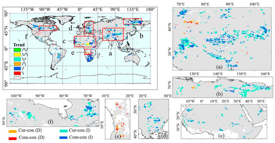
Figure 10.
(a) Distribution of annual precipitation trends between 1979 and 2016, and (b) its consistency with ESA CCI SM. (c–f) Close-up view on specific regions exhibiting consistency.
5. Conclusions
In this study, global surface soil moisture (SM) dynamics over the 1979–2016 period were documented via a non-linear methodology at both the annual and seasonal scales, based on the ESA CCI SM dataset. SM variations were classified into cubic, quadratic, linear, and insignificant trends. Non-linear trends account for about half areas of significant trends, which proves the necessity of non-linear analysis. A seasonal phenomenon was found that “wet season got wetter, and dry season got dryer”, which is more pronounced in the southern hemisphere. In addition, the difference of SM trends at various time scales revealed that SM dynamics at the seasonal scale are enhanced compared with those at the annual scale, which is seen both in terms of trend distributions and changing rate. Most seasonal dynamics which is closer to ecosystem change were concealed by annual dynamics, and seasonal change rate (ranges mainly in ±5‰ per year) is 5 times higher than the annual change rate (ranges mainly in ±1‰ per year). Despite controversial SM changes in some regions, the results based on the ESA CCI SM dataset are convincing by comparison with results of the same analysis based on the ERA-Interim reanalysis SM dataset. Overall, the non-linear trend analysis method and analysis at various time scales reveal more changes in the long-term dynamics of SM, making such a method a useful tool to get clearer understanding of environmental changes. Considering the non-linear and multi-scale characteristics of SM dynamics is necessary for relevant research and applications.
Author Contributions
Conceptualization, S.W., Y.L., and N.P.; methodology, N.P., Y.L.; data curation, N.P., Y.L.; formal analysis, visualization, and writing the original draft preparation, N.P.; writing, review and editing, N.P., Y.L.; project administration, S.W.; resources, W.Z.; supervision, B.F. All authors contributed to the writing of the manuscript.
Funding
This research was funded by the National Key Research and Development Program of China (No.2017YFA0604701), National Natural Science Foundation of China (No. 4171101213), and “the Fundamental Research Funds for the Central Universities”.
Conflicts of Interest
The authors declare no conflict of interest.
References
- Seneviratne, S.I.; Corti, T.; Davin, E.L.; Hirschi, M.; Jaeger, E.B.; Lehner, I.; Orlowsky, B.; Teuling, A.J. Investigating soil moisture–climate interactions in a changing climate: A review. Earth Sci. Rev. 2010, 99, 125–161. [Google Scholar] [CrossRef]
- Gaur, N.; Mohanty, B.P. Land-surface controls on near-surface soil moisture dynamics: Traversing remote sensing footprints. Water Resour. Res. 2016, 52, 6365–6385. [Google Scholar] [CrossRef]
- Dorigo, W.; De Jeu, R.; Chung, D.; Parinussa, R.; Liu, Y.; Wagner, W.; Fernandez-Prieto, D. Evaluating global trends (1988–2010) in homogenized remotely sensed surface soil moisture. Geophys. Res. Lett. 2012, 39, L18405. [Google Scholar] [CrossRef]
- Feng, H.; Zhang, M. Global land moisture trends: drier in dry and wetter in wet overland. Sci. Rep. 2015, 5, 18018. [Google Scholar] [CrossRef] [PubMed]
- An, R.; Zhang, L.; Wang, Z.; Quaye-Ballard, J.A.; You, J.; Shen, X.; Gao, W.; Huang, L.; Zhao, Y.; Ke, Z. Validation of the ESA CCI soil moisture product in China. Int. J. Appl. Earth Obs. Geoinf. 2016, 8, 28–36. [Google Scholar] [CrossRef]
- Li, X.; Gao, X.; Wang, J.; Guo, H. Microwave soil moisture dynamics and response to climate change in Central Asia and Xinjiang Province, China, over the last 30 years. J. Appl. Remote. Sens. 2015, 9, 096012. [Google Scholar] [CrossRef]
- Rahmani, A.; Golian, S.; Brocca, L. Multiyear monitoring of soil moisture over Iran through satellite and reanalysis soil moisture products. Int. J. Appl. Earth Obs. Geoinf. 2016, 48, 85–95. [Google Scholar] [CrossRef]
- Wang, S.; Mo, X.; Liu, S.; Lin, Z.; Hu, S. Validation and trend analysis of ECV soil moisture data on cropland in North China Plain during 1981–2010. Int. J. Appl. Earth Obs. Geoinf. 2016, 48, 110–121. [Google Scholar] [CrossRef]
- Zheng, X.; Zhao, K.; Ding, Y.; Jiang, T.; Zhang, S.; Jin, M. The spatiotemporal patterns of surface soil moisture in Northeast China based on remote sensing products. J. Water Clim. Change 2016, 7, 708–720. [Google Scholar] [CrossRef]
- Zhan, M.; Wang, Y.; Wang, G.; Hartmann, H.; Cao, L.; Li, X.; Su, B. Long-term changes in soil moisture conditions and their relation to atmospheric circulation in the Poyang Lake basin, China. Quatern. Int. 2017, 440, 23–29. [Google Scholar] [CrossRef]
- Pan, N.Q.; Feng, X.M.; Fu, B.J.; Wang, S.; Ji, F.; Pan, S.F. Increasing global vegetation browning hidden in overall vegetation greening: insights from time-varying trends. Remote Sens. Environ. 2018, 214, 59–72. [Google Scholar] [CrossRef]
- Cho, E.; Zhang, A.; Choi, M. The seasonal difference in soil moisture patterns considering the meteorological variables throughout the Korean peninsula. Terr. Atmos. Ocean. Sci. 2016, 27, 907–920. [Google Scholar] [CrossRef]
- Nie, S.; Luo, Y.; Zhu, J. Trends and scales of observed soil moisture variations in China. Adv. Atmos. Sci. 2008, 25, 43–58. [Google Scholar] [CrossRef]
- Liu, Q.; Du, J.; Shi, J.C.; Jiang, L.M. Analysis of spatial distribution and multi-year trend of the remotely sensed soil moisture on the Tibetan Plateau. Sci. China Earth Sci. 2013, 56, 2173–2185. [Google Scholar] [CrossRef]
- Yin, J.; Porporato, A.; Albertson, J. Interplay of climate seasonality and soil moisture-rainfall feedback. Water Resour. Res. 2014, 50, 6053–6066. [Google Scholar] [CrossRef]
- Zhang, H.; Chang, J.; Zhang, L.; Wang, Y.; Li, Y.; Wang, X. NDVI dynamic changes and their relationship with meteorological factors and soil moisture. Environ. Earth Sci. 2018, 77, 582. [Google Scholar] [CrossRef]
- Bai, W.K.; Gu, X.L.; Li, S.L.; Tang, Y.H.; He, Y.H.; Gu, X.H.; Bai, X.Y. The performance of multiple model-simulated soil moisture datasets relative to ECV satellite data in China. Water 2018, 10, 1384. [Google Scholar] [CrossRef]
- Qiu, J.; Gao, Q.; Wang, S.; Su, Z. Comparison of temporal trends from multiple soil moisture data sets and precipitation: The implication of irrigation on regional soil moisture trend. Int. J. Appl. Earth Obs. 2016, 48, 17–27. [Google Scholar] [CrossRef]
- Chen, X.; Su, Y.; Liao, J.; Shang, J.; Dong, T.; Wang, C.; Liu, W.; Zhou, G.; Liu, L. Detecting significant decreasing trends of land surface soil moisture in eastern China during the past three decades (1979–2010). J. Geophys. Res. Atmos. 2016, 121, 5177–5192. [Google Scholar] [CrossRef]
- Teuling, A.J.; Hupet, F.; Uijlenhoet, R.; Troch, P.A. Climate variability effects on spatial soil moisture dynamics. Geophys. Res. Lett. 2007, 34, L06406. [Google Scholar] [CrossRef]
- Gabiri, G.; Burghof, S.; Diekkrüger, B.; Leemhuis, C.; Steinbach, S.; Näschen, K. Modeling spatial soil water dynamics in a tropical floodplain, East Africa. Water 2018, 10, 191. [Google Scholar] [CrossRef]
- Lekshmi, S.U.S.; Singh, D.N.; Baghini, M.S. A critical review of soil moisture measurement. Measurement 2014, 54, 92–105. [Google Scholar]
- Petropoulos, G.P.; Ireland, G.; Barrett, B. Surface soil moisture retrievals from remote sensing: Current status, products & future trends. Phys. Chem. Earth. 2015, 3, 36–56. [Google Scholar]
- Catalano, F.; Alessandri, A.; de Felice, M.; Zhu, Z.; Myneni, R.B. Observationally based analysis of land–atmosphere coupling. Earth Syst. Dynam. 2016, 7, 251–266. [Google Scholar] [CrossRef]
- Knist, S.; Goergen, K.; Buonomo, E.; Christensen, O.B.; Colette, A.; Cardoso, R.M.; Fealy, R.; Fernández, J.; García-Díez, M.; Jacob, D.; Kartsios, S.; et al. Land-atmosphere coupling in EURO-CORDEX evaluation experiments. J. Geophys. Res. 2017, 122, 79–103. [Google Scholar] [CrossRef]
- Li, M.; Ma, Z.; Gu, H.; Yang, Q.; Zheng, Z. Production of a combined land surface data set and its use to assess land-atmosphere coupling in China. J. Geophys. Res. 2017, 122, 948–965. [Google Scholar] [CrossRef]
- Carvalhais, N.; Forkel, M.; Khomik, M.; Bellarby, J.; Jung, M.; Migliavacca, M.; Μu, M.Q.; Saatchi, S.; Santoro, M.; Thurner, M.; et al. Global covariation of carbon turnover times with climate in terrestrial ecosystems. Nature 2014, 514, 213–217. [Google Scholar] [CrossRef]
- Richardson, A.D.; Keenan, T.F.; Migliavacca, M.; Ryu, Y.; Sonnentag, O.; Toomey, M. Climate change, phenology, and phenological control of vegetation feedbacks to the climate system. Agric. For. Meteorol. 2013, 169, 156–173. [Google Scholar] [CrossRef]
- Dobriyal, P.; Qureshi, A.; Badola, R.; Hussain, S.A. A review of the methods available for estimating soil moisture and its implications for water resource management. J. Hydrol. 2012, 458, 110–117. [Google Scholar] [CrossRef]
- Wanders, N.; Karssenberg, D.; de Roo, A.; de Jong, S.M.; Bierkens, M.F.P. The suitability of remotely sensed soil moisture for improving operational flood forecasting. Hydrol. Earth Syst. Sci. 2014, 18, 2343–2357. [Google Scholar] [CrossRef]
- Asoka, A.; Gleeson, T.; Wada, Y.; Mishra, V. Relative contribution of monsoon precipitation and pumping to changes in groundwater storage in India. Nat. Geosci. 2017, 10, 109–117. [Google Scholar] [CrossRef]
- Park, S.; Im, J.; Park, S.; Rhee, J. Drought monitoring using high resolution soil moisture through multi-sensor satellite data fusion over the Korean peninsula. Agric. For. Meteorol. 2017, 237, 257–269. [Google Scholar] [CrossRef]
- Nicolai-Shaw, N.; Zscheischler, J.; Hirschi, M.; Gudmundsson, L.; Seneviratne, S.I. A drought event composite analysis using satellite remote-sensing based soil moisture. Remote Sens. Environ. 2017, 203, 216–225. [Google Scholar] [CrossRef]
- Mishra, A.; Vu, T.; Valiya, V.A.; Entekhabi, D. Drought monitoring with soil moisture active passive (SMAP) measurements. J. Hydrol. 2017, 552, 620–632. [Google Scholar] [CrossRef]
- Dorigo, W.; Wagner, W.; Albergel, C.; Albrecht, F.; Balsamo, G.; Brocca, L.; Chung, D.; Ertl, M.; Forkel, M.; Gruber, A. ESA CCI Soil moisture for improved earth system understanding: State-of-the art and future directions. Remote Sens. Environ. 2017, 203, 185–215. [Google Scholar] [CrossRef]
- Liu, Y.X.; Wang, Y.L.; Du, Y.Y.; Zhao, M.Y.; Peng, J. The application of polynomial analyses to detect global vegetation dynamics during 1982–2012. Int. J. Remote. Sens. 2016, 37, 1568–1584. [Google Scholar] [CrossRef]
- Tian, L.F.; Collins, C. An effective robot trajectory planning method using a genetic algorithm. Mechatronics 2004, 14, 455–470. [Google Scholar] [CrossRef]
- Feng, H.H. Individual contributions of climate and vegetation change to soil moisture trends across multiple spatial scales. Sci. Rep. 2016, 6, 32782. [Google Scholar] [CrossRef]
- Piao, S.; Yin, L.; Wang, X.; Ciais, P.; Peng, S.; Shen, Z.; Seneviratne, S.I. Summer soil moisture regulated by precipitation frequency in China. Environ. Res. Lett. 2009, 4, 044012. [Google Scholar] [CrossRef]
- Chen, X.; Liu, X.; Liu, Z.; Zhou, P.; Zhou, G.; Liao, J.; Liu, L. Spatial clusters and temporal trends of seasonal surface soil moisture across China in responses to regional cli-mate and land cover changes. Ecohydrology 2017, 10, 1–12. [Google Scholar]
- Meng, X.; Li, R.; Luan, L.; Lyu, S.; Zhang, T.; Ao, Y.; Han, B.; Zhao, L.; Ma, Y. Detecting hydrological consistency between soil moisture and precipitation and changes of soil moisture in summer over the Tibetan Plateau. Clim. Dyn. 2017, 2, 1–12. [Google Scholar] [CrossRef]
© 2019 by the authors. Licensee MDPI, Basel, Switzerland. This article is an open access article distributed under the terms and conditions of the Creative Commons Attribution (CC BY) license (http://creativecommons.org/licenses/by/4.0/).