Article

Drought Assessment in a Semi-Arid River Basin in China and its Sensitivity to Different Evapotranspiration Models

MOE Key Laboratory of Groundwater Circulation and Environmental Evolution, School of Water Resources and Environment, China University of Geosciences (Beijing), Beijing 100083, China
*
Author to whom correspondence should be addressed.
Water 2019, 11(5), 1061; https://doi.org/10.3390/w11051061
Submission received: 16 April 2019 / Revised: 14 May 2019 / Accepted: 19 May 2019 / Published: 22 May 2019
(This article belongs to the Section Hydrology)

Abstract

:
The Standardized Precipitation Evapotranspiration Index (SPEI) is widely used for climatological and hydrological studies, in which the estimation of potential evapotranspiration (PET) is of great importance. As many different models exist in estimating PET, the question that arises is in which way the selection of the PET model affects the calculated SPEI and the drought assessment. This study, on the basis of evaluating drought conditions over the Hexi Inland River Basin in China with long-term climate data of 18 stations by using SPEI, compared three types and eight kinds different PET models with respect to their sensitivity to the calculation of SPEI, and to drought events and drought characteristics. The results showed that the study area experienced a drying trend over the past 56 years, and the extreme drought events occurred more frequently after 2000 as a whole. All the investigated PET models were sensitive to the estimation of SPEI and to the drought assessment. When considering the alternatives of the Thornthwaite model in the calculation of SPEI for drought identification, the Blaney–Criddle equation among the temperature-based models and the Makkink equation among the radiation-based models are recommended due to the comparable results in determining the drought trends, drought events, and drought characteristics.

1. Introduction

Drought is one of the major natural disasters in human history, and its catastrophic consequences are still innumerable even with current highly developed science and technology. Generally speaking, drought is usually divided into these categories: Meteorological drought, hydrological drought, agricultural drought, and socio-economic drought [1,2,3]. Among these types, meteorological drought is usually the basis for the other three types of droughts. When the meteorological drought persists for a period of time, other types of droughts occur with corresponding consequences. Therefore, timely meteorological drought monitoring is essential for early warning and risk management of water resources and agricultural production [4]. Furthermore, drought assessment is of great importance for water resource planning and management [5], and it can help governments to develop a more proactive approach to drought management and planning [6], especially for regions prone to drought.
The trend of aridization has become a global concern [7], especially for drought-prone regions. The Hexi Inland River Basin is located in the northwest of China. Due to its geographical location, its climate is typically continentally arid with little precipitation. It is a drought prone region due to the shortage of water resources. Some of the drought events in its history include the drought that spanned during 1960–1963 and 1980–1990. The 1995–2000 drought that followed also became one of the most notable natural hazardous events the basin had ever encountered. Sandstorms that result from droughts also cannot be ignored. A large-scale strong sandstorm occurred in May 1993 for example, causing considerable casualties and economic losses in the basin. The occurrence of heavy sandstorms increased to more than 20 times in the 1990s from five times in the 1950s [8]. Drought assessment in the basin can not only provide support for drought mitigation and drought management and planning, but also is of great importance for local water resource allocation and management to maintain a favorable ecological environment.
Various drought indices have been used to understand meteorological drought, such as percent normal or deciles of precipitation [9], Multivariate Standardized Drought Index (MSDI) [10], Standardized Soil Moisture Index (SSMI) [10], Palmer Drought Severity Index (PDSI) [11], Standardized Precipitation Index (SPI) [12], and Standardized Precipitation Evapotranspiration Index (SPEI) [13], etc. The most commonly used meteorological drought index is SPEI which combines the sensitivity of PDSI to changes in evaporation demand and the multi-temporal nature of the SPI [13]. Although this index requires only climatological information without assumptions about the characteristics of the underlying system, it is more useful and has been widely used for climate change studies due its consideration of information about temperature [14,15,16,17]. It also has been proved to be particularly suitable for detecting, monitoring, and exploring the consequences of global warming on drought conditions [18,19,20,21,22].
The SPEI is designed to take into account both precipitation and potential evapotranspiration (PET) data in determining drought [13]. Thus, the derivation of PET data is of great importance in the estimation of SPEI. Vicente-Serrano et al. [13] originally suggested the use of the simple Thornthwaite (TH) [23] equation for the estimation of PET, which only requires mean daily temperature and latitude of the site, whilst the variables affecting PET such as wind speed, surface humidity, and solar radiation are not accounted for. Many scholars like Donohue et al. [24], Van der Schrier et al. [25], and Sheffield et al. [26] found that in some cases the PET value cannot be accurately estimated by using the TH equation, underestimated in arid and semiarid regions, and overestimated in humid and tropical regions [27,28]. Some scholars suggest that a more sophisticated method to calculate PET is often preferred in order to make a more complete accounting of drought variability in cases where more data are available [29,30]. Yuan and Quiring [31] estimated the PET by using three models: Penman–Monteith equation, the two-source PET equation, and the TH equation in calculating the Palmer Drought Severity Index and then evaluated how PET affected the drought conditions of the Great Plains from 1980 to 2012. Zhang et al. [32] also investigated the sensitivity of the above three models in drought monitoring by using SPEI. Although the issue of using different evapotranspiration models has been evaluated and suggested in many previous studies of estimating drought index, there is still much disagreement on the selection of PET models due to various study areas and study purposes [33,34,35]. Hence, more research is still needed to enrich the related results, especially on local scales.
The objectives of this paper are firstly to evaluate the drought conditions in the Hexi Inland River Basin in China with SPEI, employing the TH equation for PET calculation, and then examining the sensitivities of different PET models to SPEI and to drought assessments. The study period spanned from 1960 to 2015. The study tried to find in which way the selection of PET model affected the calculated SPEI and the drought assessments. In particular, as many as three types and eight kinds of PET models were employed, including four temperature-based models, Thornthwaite, Blaney–Criddle, Hamon and Szász, two radiation-based models of Makkink and Priestley–Taylor, and two combination models of Penman and Penman–Monteith for comparative analysis.

2. Study Area and Methods

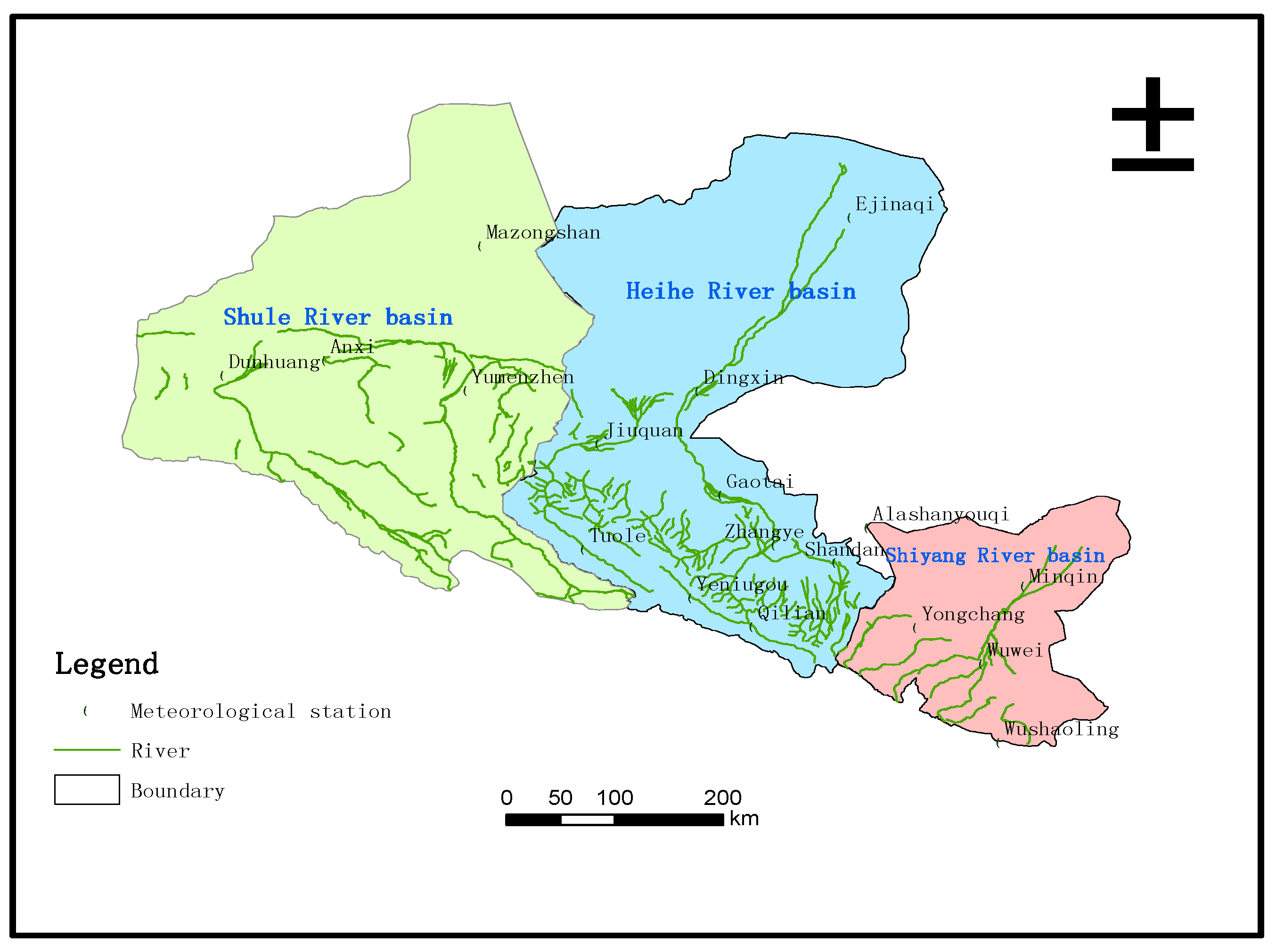
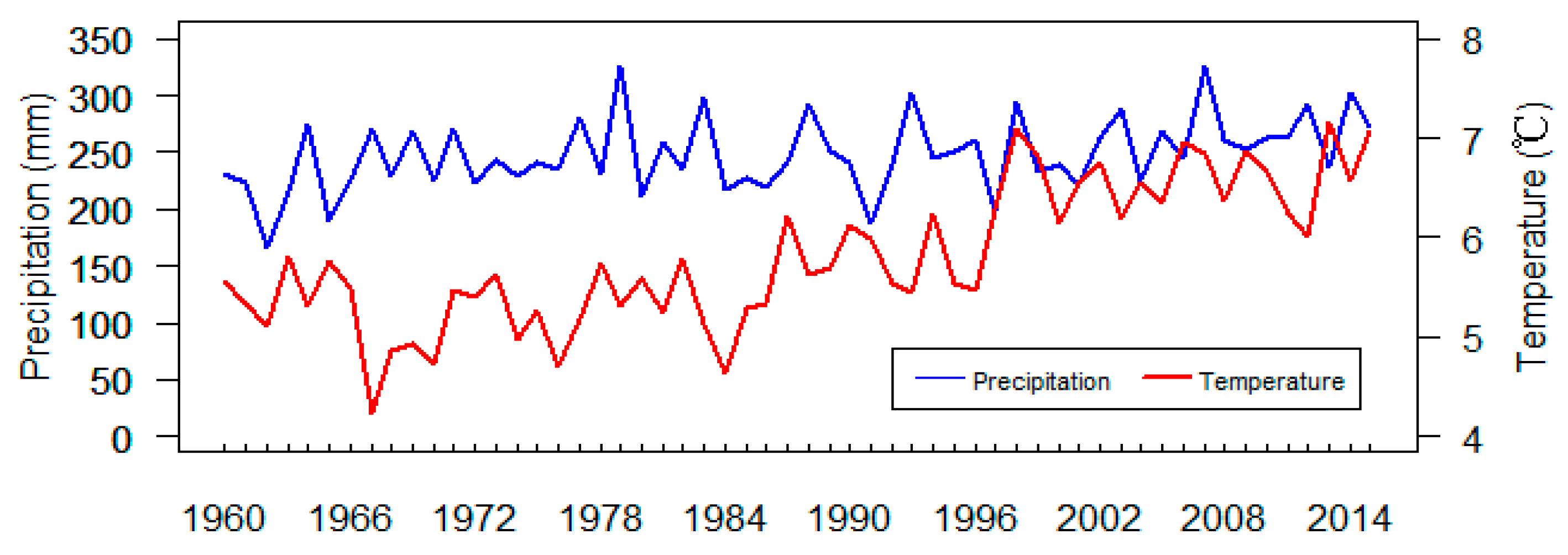
2.1. Study Area and Data Description

The Hexi Inland River Basin (HIRB) is located in the northwest of China, covering an area of approximately 27.11 × 10⁴ km2, within the range of 37°17’–42°48’ N and 93°23’–104°12’ E. It has a typical continental arid climate with an annual mean precipitation of 248 mm, gradually decreasing from east to west. The annual mean temperature over the basin is 5.8 °C, increasing from the mountainous to the plain, with strong evaporation that amounts to 1095 mm on average. Both the temperature and the evaporation show great differences between day and night. The whole basin is divided into three major river basins: the Shiyang River Basin (SYRB), Heihe River Basin (HRB), and Shule River Basin (SLRB) from east to west.
There are 23 national meteorological stations over the study area in total, with some of the stations missing data. Whilst considering the data integrity and data quality, 18 stations within a 56-year period (from 1960 to 2015) were selected, in which five of them (Wushaoling (WSL), Yongchang (YC), Wuwei (WW), Alashanyouqi (ALSYQ), Minqin (MQ)) are located in SYRB. Nine (Tuole (TL), Yeniugou (YNG), Qilian (QL), Shandan (SD), Zhangye (ZY), Jiuquan (JQ), Gaotai (GT), Dingxin (DX), Ejinaqi (EJNQ)) are located in HRB, and four (Mazongshan (MZS), Yumenzhen (YMZ), Anxi (AX), Dunhuang (DH)) in SLRB. The locations of the meteorological stations are shown in Figure 1. The daily observed datasets consisting of temperature, precipitation, relative humidity, wind speed, and sunshine hours are freely available from the China Meteorological Data Network (https://data.cma.cn/). The detailed information of the selected stations is shown in Table 1. Figure 2 shows the time-series of 12-month areal annual precipitation (in blue) and the annual mean temperature (in red) over the HIRB for the last 56 years. The areal precipitation and temperature were calculated by using arithmetic average method. According to Figure 2, there have been comparatively small fluctuations without clear trends in areal annual precipitation, while substantial climate warming presented with the areal annual temperature increased by 1.51 °C from 1960 to 2015. The precipitation and temperature patterns over the study area play important roles in the occurrence of droughts.

2.2. SPEI and Drought Characteristics

The SPEI is a simple multi-scalar drought index that combines temperature and precipitation data. It is based on the original SPI calculation procedure. Firstly, use the TH [23] equation to calculate the monthly potential evapotranspiration (PET) (mm); then calculate the difference between the precipitation (P) and PET for the month i using the formula D i = P i PET i . Lastly, choose the Log-logistic distribution to model D i values, and the resulting cumulative probabilities are transformed into a standardized variable [13]. Detailed descriptions of the SPEI calculation can be found in the references of Vicente–Serrano et al. [13], Beguería et al. [30], and Um et al. [36]. In this study, we analyzed the SPEI series at a 12-month scale, which represented the accumulated water deficits of 12 months and reflected the inter-annual variation of drought.
The drought was divided into five levels according to the estimated SPEI values based on National Meteorological Drought Rating Standard [37], which is shown in Table 2. When the SPEI values showed less than or equal to −0.5, it was regarded as a drought event. Three characteristics, drought duration, drought severity, and drought peak, were defined and derived from a drought event according to the Run theory [38]. Drought duration means the total duration of a drought event. According to the regional drought identification results, if the study area continues from the i time period to the i + T period, the drought event lasts for T. Drought severity means the weighted sum of the drought intensity areas of each drought assessment unit at each time interval in a drought duration. Drought peak means the minimum SPEI value of a drought event, which is the extreme value of a negative run [38].

2.3. Calculations of PET

The SPEI only considers P and PET when determining droughts. Therefore, the derivation of PET data is very important in the estimation of SPEI. Models for PET estimations can be grouped into such categories as temperature-based, radiation-based, combination, mass-transfer, etc. [39]. The temperature-based method refers to those where only temperature is required as the input variable in the estimation of PET, including Thornthwaite [23], Blaney–Criddle [40], Hargreaves and Samani [41], Kharrufa [42], Hamon [43], and Szász [44] models. Radiation-based models based on the energy balance includes Makkink [45], Hargreaves [46], Abtew [47], and Priestley and Taylor [48]. Combination model considers the influence of aerodynamics and requires more input parameters and a more complicated calculation process. It includes the commonly used Penman [49] and Penman–Monteith [29] models. The mass-transfer model based on Dalton’s evaporation law takes the influence of wind, temperature, humidity, and other meteorological factors on evaporation into account [39].
In general, the selection of appropriate PET models in a given study depends on research purposes, as well as the availability of climatic input data and the local climate conditions. In this study, three types, eight kinds of evapotranspiration models were selected for comparative analysis, namely the temperature-based Thornthwaite (TH), Blaney–Criddle (BC), Hamon and Szász, the radiation-based Makkink, and Priestley–Taylor (PT), as well as the combination models of Penman and Penman–Monteith (PM). A detailed description of each model is summarized in Table 3.

3. Results and Analysis

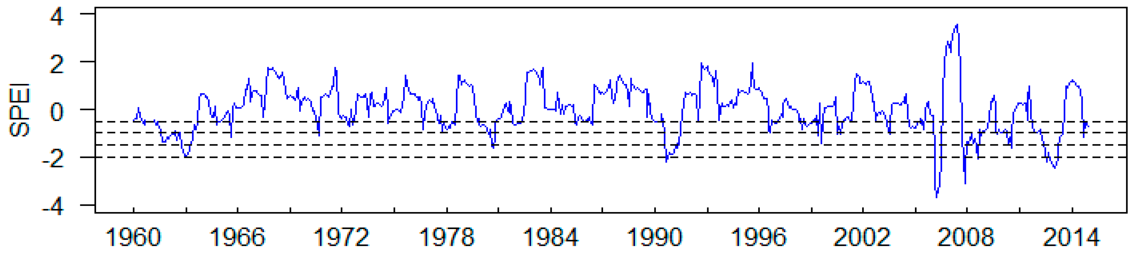
3.1. Drought Assessment over the Study Area

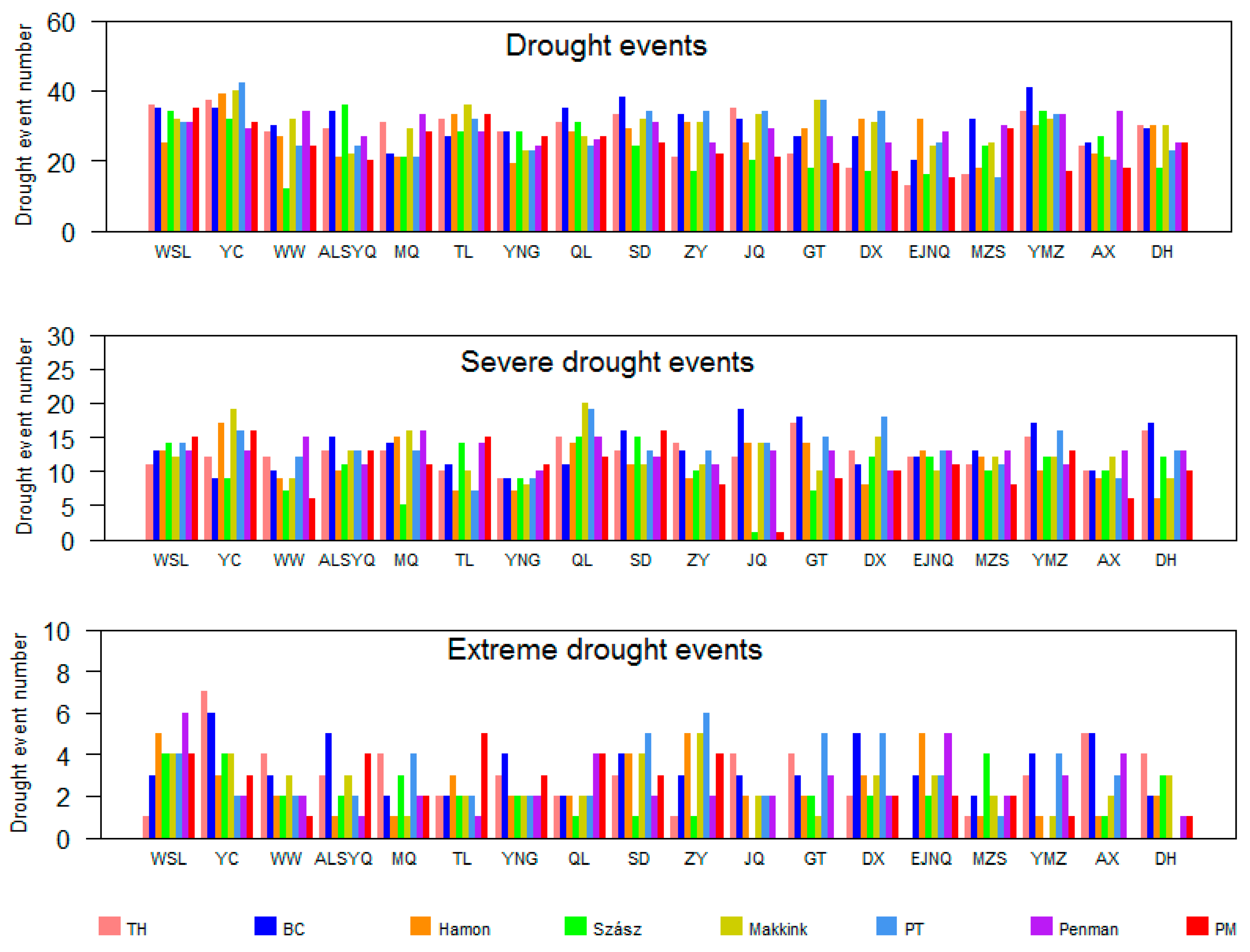
3.1.1. Drought Events

The drought conditions were determined according to the criteria mentioned in Section 2.2, that when the SPEI value for a particular time period fell less than or equal to −0.5, it was regarded as a drought event. Due to limited space, taking YC station as an example, Figure 3 shows the SPEI series obtained by the TH equation. Four dotted lines from top to bottom in the figure represent the thresholds of four drought levels: Light, moderate, severe, and extreme droughts, respectively. Table 4 summarizes the total number of drought events and the number of drought events after 2000, together with the number of severe and extreme drought levels for all stations.
From Figure 3 and Table 4, we can see that 37 drought events occurred during the period of 1960–2015 for YC station, and 32% (12 of 37) of them occurred after 2000. As to the different drought levels, more numbers of severe and extreme drought events occurred after 2000 (Figure 3), specifically 50% (6 of 12) severe and 71% (5 of 7) extreme events occurred after 2000 (Table 4).
Across all stations of the study area, the drought event numbers ranged from 13 to 37 from 1960 to 2015, and 11 stations (61%) experienced more than 40% drought events after 2000. As to the different levels, 14 stations (78%) experienced more than 50% severe and extreme drought events during the period of 1960 to 2015. In particular, 10 stations experienced no extreme droughts before 2000, and all extreme droughts occurred after 2000, which means that the extreme drought events occurred more frequently after 2000 for most stations as a whole.
From Table 4, it also can be concluded that 15 of 18 (83%) stations experienced drought events for every 3 years on average as a whole (≥18.7 drought events during the 56 years), and 12 of 18 (67%) stations experienced drought events for every 2 years (≥28 drought events during the 56 years), and YC station experienced the most frequent drought events with the occurrence of every 1.5 years on average.
In order to assess the changes of drought events over time, trend analysis of the drought event series was performed by using the widely used non-parametric Mann–Kendall (MK) test [50]. The second row in Table 5 shows the statistic Z values from the MK test for all stations. It indicates that, 16 of 18 stations experienced decreasing trends, and such trends were significant for 15 of them at 0.05 significance level. It means that most stations across the basin experienced significant drying trends over the past several years.

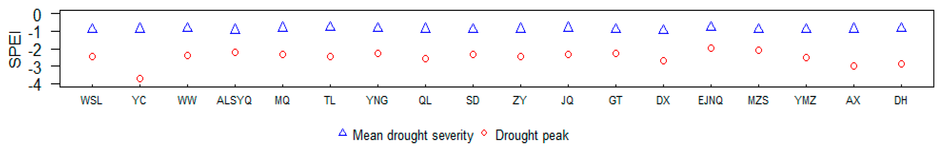
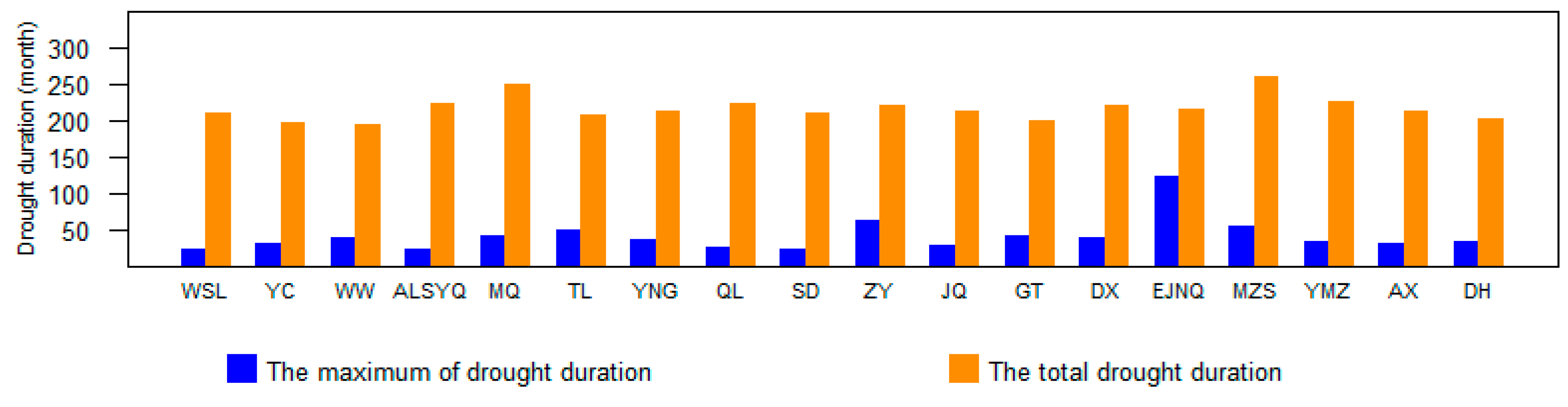
3.1.2. Drought Characteristics

Figure 4 and Figure 5 show the statistics of the three drought characteristics based on the Run theory. The mean drought severity ranges from −0.79 and −0.96, belonging to light drought level, and are presented very close to each other for all stations, while great differences are found for the drought peak varying from −1.99 and −3.68, in which YC station experienced the highest drought peak (in March 2007), 1.2–1.8 times to other stations (Figure 4). As for the drought duration, we counted the total duration, as well as the maximum duration of drought events for all stations during the period of 1960 to 2015 (Figure 5). It ranged from 194 to 260 months for total duration, with an average of 216 months across the basin, in which MZS and MQ stations ranked as the first two with the longest total drought duration. The maximum drought duration varied greatly across the basin, from 22 to 123 months. It should be noted that EJNQ station, although it experienced the least numbers of drought events (13 times) with nearly none at the extreme level (Table 4), showed a minimum drought peak of −1.99 (Figure 4) and had the longest drought duration of up to 123 months (more than 10 years) (Figure 5), occurring from June 2005 to August 2015. Such long-term drought duration inevitably led to the deterioration of the ecological environment and social economy.
In summary, the above results demonstrated that the drought events in the basin occurred every 2–3 years on average, during 1960–2015, with more than 40% of drought events occurring after 2000 for 61% stations. Among all drought events, the extreme drought events occurred more frequently after 2000 as a whole. By performing the Mann–Kendall trend test on the drought event series, we found that the trend of drought was aggravating for the whole basin which coincided with the rise in temperature. It should be noted that the drought peak and the maximum drought duration presented great spatial heterogeneity.

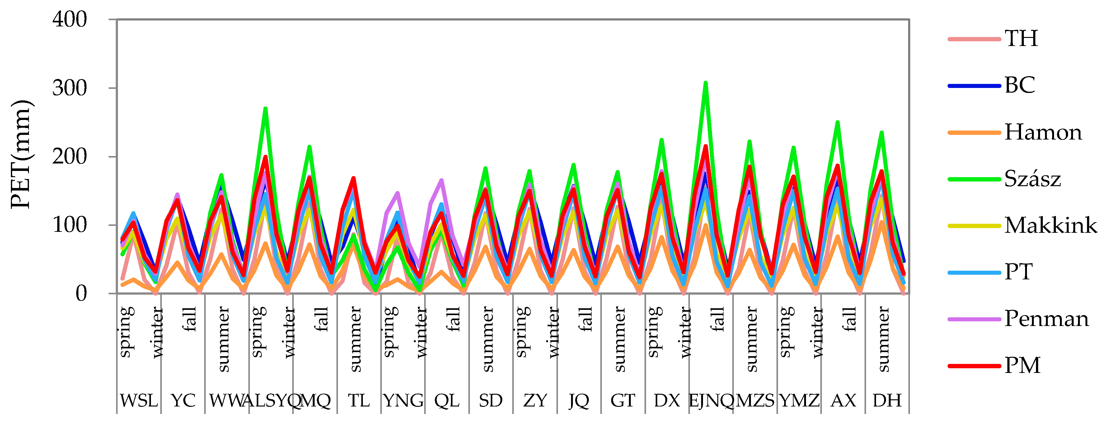
3.2. Comparison of PET Models

The annual average PET values calculated from different models for the study area are given in Table 6. For comparison, we took the PET values from the TH model as the benchmark. The annual average PET from the benchmark was 581 mm for the basin. Quite substantial differences were found in PET values from various models. The temperature-based Hamon model always brought less PET values, an average of 62% lower than that from the benchmark. The other six equations always brought larger PET values. Among them, temperature-based BC and Szász have the highest overall PET values, which were twice the benchmark on average. The combination methods of Penman and PM give quite close PET values for all stations, 1.9 times larger than the benchmark on average across the basin. In contrast, PET values from the radiation-based Makkink and PT were closest to the benchmark (1.4–1.6 times the benchmark on average).
Figure 6 shows the intra-annual distribution of PET values. Similar seasonal variations in PET values are found from different models for most parts of the study area; uneven intra-annual distributions with initially increasing and then decreasing from January to December with an occurring maximum value in July. Compared with the benchmark TH model, five of the other models (BC, Szász, PT, Penman, and PM) presented higher values no matter the month and season as a whole, in which Szász gave the highest values during the middle of the year (from April to September) for most stations. Makkink presented similar values with the benchmark during the summer season (June, July, and August) and higher values during the other seasons. Hamon gave much lower PET values during the period of April to September. Comparatively, the intra-annual distribution curves from Penman and PM overlap the most. It should be noted that PET values derived from the benchmark equation were near to zero during the winter season (January, February, and December), which was mainly due to the fact that when the temperature was below 0 °C, the PET calculated by TH was equal to zero.

3.3. Effects of Different PET Models to SPEI

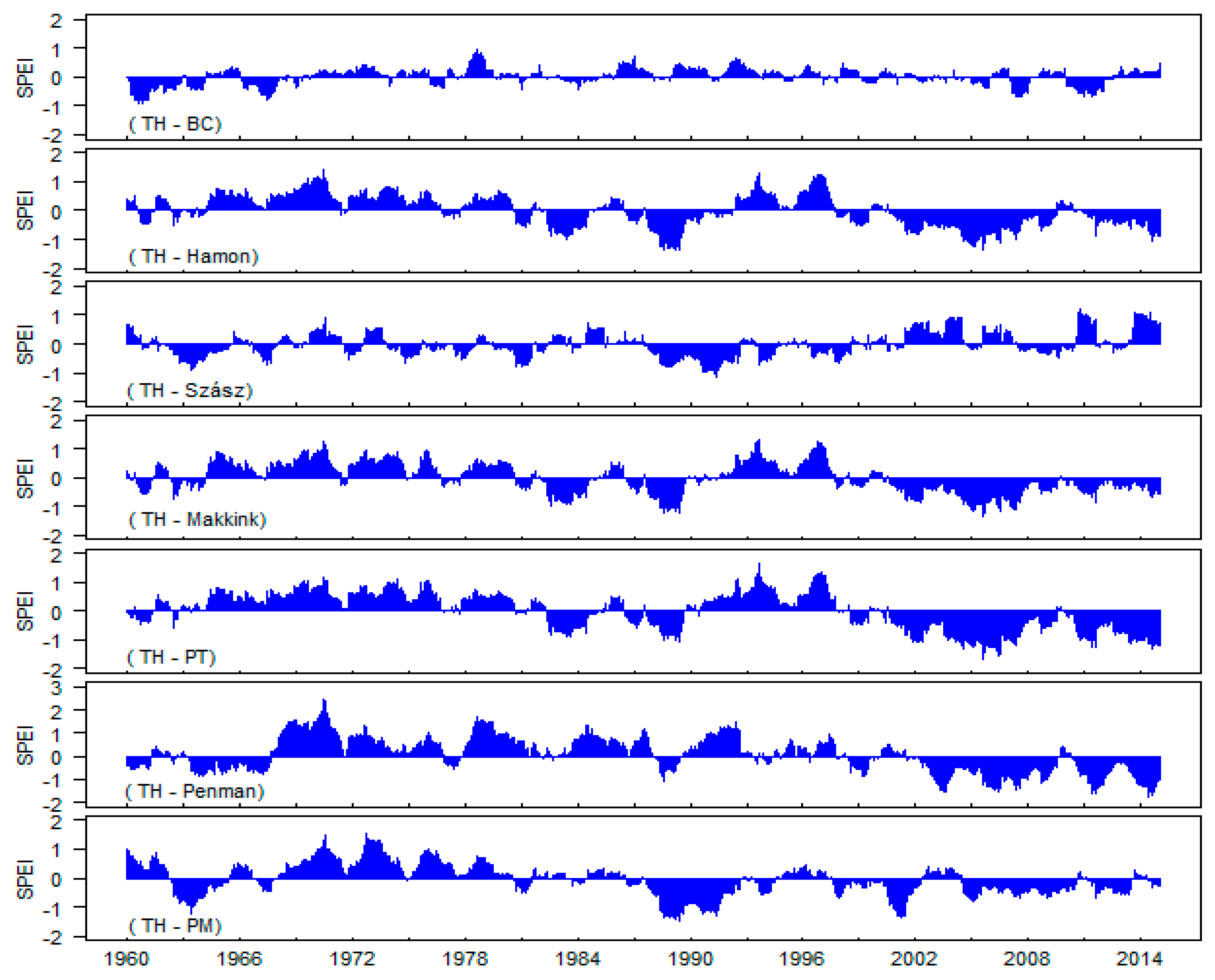
3.3.1. SPEI Differences from Various PET Models

For clarity, the PET model is written as the subscript of SPEI. For instance, the SPEI values obtained from the TH model is written as SPEITH. Differences between SPEITH and the SPEI from other alternative PET models are firstly examined, and Figure 7 shows such differences with YC station as an example. It can be seen that the difference between SPEITH and SPEIBC presents the smallest within the range of 1 unit, and the difference between SPEITH and SPEISzász presents the second smallest, indicating that SPEIBC, SPEISzász are very close to SPEITH. These almost identical patterns are found in the plots of TH–Hamon, TH–Makkink, and TH–PT, having nearly two remarkable positive differences (from 1964 to 1982 and from 1991 to 1999), and two remarkable negative differences (from 1982 to 1991 and after 1999), and about 93% of the differences are within 1 unit. The patterns for plots of TH–Penman and TH–PM are similar for most of the years. SPEIPenman is close to SPEIPM, while both of them differ greatly from SPEITH with larger difference ranges.
For other stations, similar conclusions can be drawn that SPEIBC, SPEISzász are similar to SPEITH, with nearly similar patterns found in the plots of TH–Makkink, TH–PT, and TH–Hamon. Furthermore, the differences between SPEITH and SPEIPenman (or SPEIPM) are relatively large. It can also be concluded that the SPEITH identified more climate drying trends than other SPEI series since the differences between them always change from positive values to negative values over time as a whole.

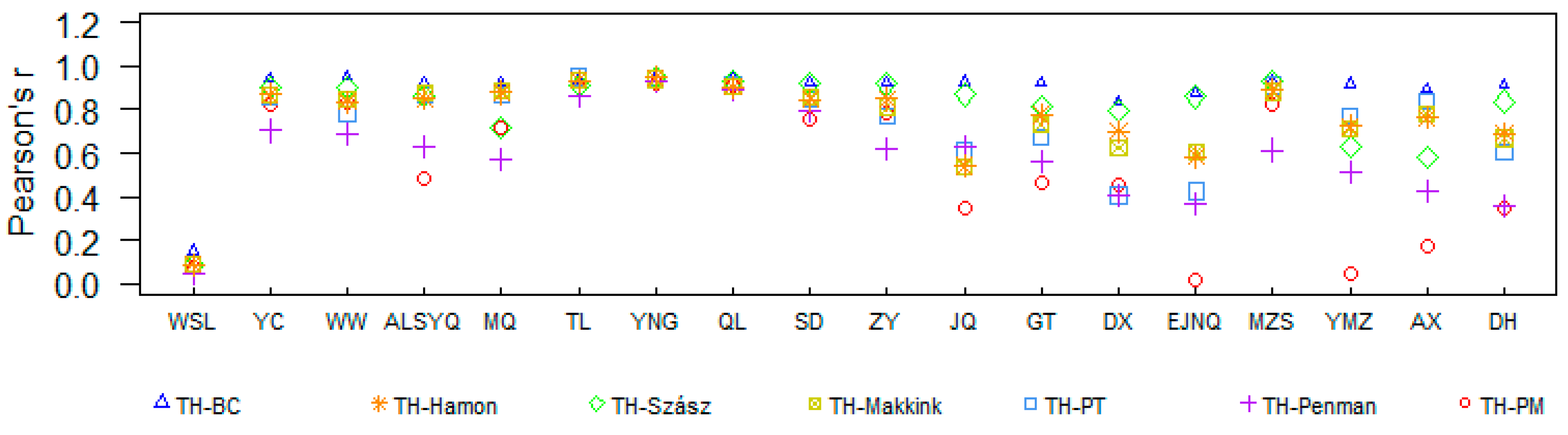
3.3.2. SPEI Correlation Analysis

SPEI values from different PET models were also compared by using the Pearson correlation coefficient. Figure 8 shows the correlation coefficients of the eight SPEI series for all stations. It indicates that SPEITH and SPEIBC are the most correlated with correlation coefficients greater than 0.93 (at 17 of 18 stations). The highest correlations between them demonstrate that these equations produce quite comparable SPEI values for drought assessment.
Comparing the correlation coefficients for each station, we found that SPEIBC, SPEISzász, and SPEIHamon ranks the first three as the most correlated with SPEITH for 18 stations, followed by SPEIPT and SPEIMakkink. The poorest correlations are observed between SPEITH and SPEIPM, and a similar weak correlation for SPEITH and SPEIPenman can be seen. Overall, SPEITH are most correlated with the SPEI derived from the temperature-based PET model, followed by those from the radiation-based model. The SPEI from the comprehensive-based models have poorest correlations with SPEITH.

3.3.3. Drought Events

Through previous analysis, we know that there are some differences in SPEI values derived from different PET models. Figure 9 shows the number of drought events and number of severe and extreme drought events for all stations. On average, the BC model produced more drought event numbers, followed by the Makkink, Penman, and PT models. Hamon and TH produced close drought event numbers, while Szász and PM produced less drought event numbers comparatively. As for the severe and extreme drought events, different results are found. BC, as well as the PT models still overestimated the drought event numbers, while Makkink and Penman produced close numbers with TH, while Szász, PM, and Hamon tended to underestimate the drought event numbers.
To evaluate whether the tendency of drought events occurrence remained consistent from different SPEI series, trend analysis was performed on the seven SPEI series by using the MK test. Table 5 shows the results of trend analysis for all stations. It can be seen that, although the use of different equations for calculating SPEI leads to great differences in the magnitude of the trends, SPEIBC kept quite a consistent decreasing trend with SPEITH for most stations. SPEIMakkink ranked next, keeping consistent decreasing trends with SPEITH for 14 of 18 stations, SPEISzász and SPEIPT ranked third, showing decreasing trends as SPEITH for 13 of 18 stations. SPEIPenman deviated most from SPEITH with many stations presenting opposite increasing trends. According to SPEIPenman, 12 of 18 stations were detected to experience increasing trends (wetting trends) during the period of 1960 to 2015.

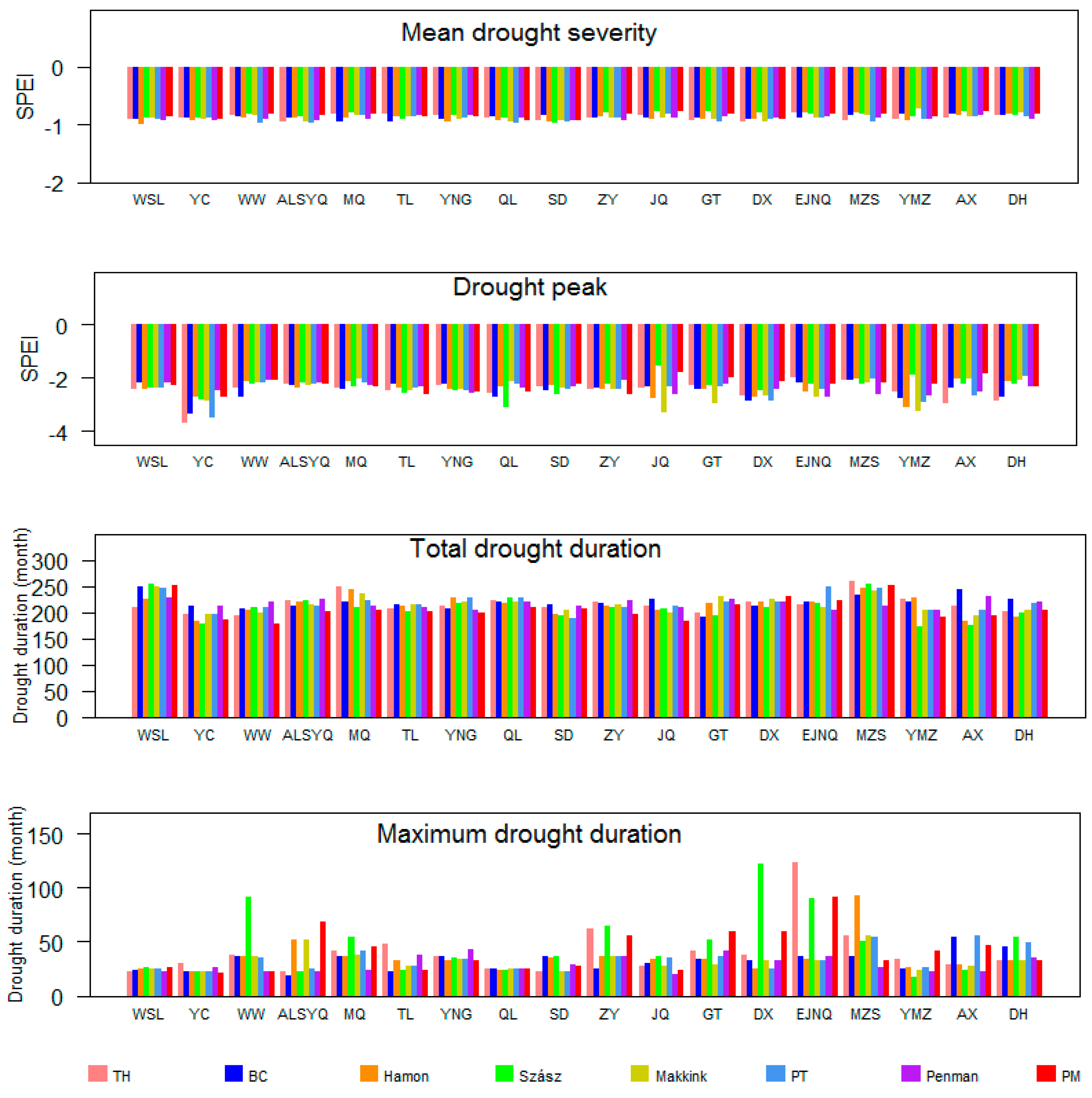
3.3.4. Drought Characteristics

For a better understanding of the effects of different PET models to drought characteristics, we compared the drought severity, drought duration, and drought peak derived from the different SPEI series based on the Run theory, with the results shown in Figure 10. The mean drought severity extracted from the different SPEI series were basically close to each other at all stations, ranging from −0.73 to −0.99, and all belonging to the light drought level. As for the drought peak, results from BC, PT, and PM were in good agreement with TH, all showing the largest drought peak at YC station although the peak value differed a little (−3.34, −3.50, −2.73, and −3.68 for BC, PT, PM, and TH). Another point was that most of the drought peak derived from Penman and PM were smaller than those from other models, indicating that the drought detected from these two equations was not as serious as those from other models.
As for drought duration, Hamon, Makkink, and Penman produced the closest drought duration with TH (216 months), comparatively. BC and PT produced a slightly longer drought duration with an average of more than 218 months across the basin, while Szász and PM usually produced a shorter drought duration with an average of 207 months. As for maximum drought duration, BC, Makkink, PT, and Penman gave relatively close results across the basin, ranging from 19–54 months, 23–55 months, 23–55 months, and 20–43 months, respectively, without detecting very long drought duration for all stations. Szász and PM produced a similar result with the TH model, detecting the longest drought duration occurring at EJNQ station, 122 and 92 months, respectively, although the duration, especially from the PM model, did not last as long as TH detected.
We estimated the SPEI from as many as eight PET models and compared the SPEI series from the perspectives of the difference, the correlation, the number, and trend of drought events and drought characteristics. As a result, the comparative application of the different PET models in SPEI revealed that the drought assessment was sensitive to the selection of the PET model, while the sensitivities could not be totally grouped in terms of different types of PET models. SPEIBC and SPEISzász were most close to SPEITH, while SPEIPenman and SPEIPM differed greatly from SPEITH. SPEITH had good correlations with SPEI derived from the temperature-based PET models, followed by those from the radiation-based models, partly keeping consistent with the findings of trend analysis. SPEIBC (temperature-based) showed a strong drying trend as SPEITH, followed by SPEIMakkink (radiation-based), SPEISzász (temperature-based), and SPEIPT (radiation-based).
We also tried to seek some alternatives to PET models so as to improve the flexibility of SPEI. According to our study, among the temperature-based equations, SPEIBC and SPEITH were the most correlated, with the smallest difference, and keeping a quite consistent decreasing trend for most stations. Furthermore, BC could give similar results to TH for drought peak and drought severity. High consistency in these aspects demonstrated that the BC model could be regarded as one alternative to TH in the estimation of SPEI. As for the radiation-based models, Makkink provided similar results to TH in drought severity, total drought duration, and severe and extreme drought event numbers. Meanwhile, SPEIMakkink kept largely consistent decreasing trends with SPEITH. Thus, Makkink was capable of being regarded as the alternative one among the radiation-based models. Comparatively, SPEIPenman and SPEIPM deviated most from SPEITH in many aspects.

4. Conclusions

This paper evaluated drought conditions over the Hexi Inland River Basin by employing the drought index of SPEI and investigating the effects of different PET models to SPEI and to drought assessments. In summary, the result confirmed that the extreme drought events occurred more frequently after 2000 as a whole across the study area and the trend of drought is still aggravating. The estimation of SPEI and the drought assessment were sensitive to the selection of PET models we used. The BC equation is suggested as an alternative in estimating PET and the follow-up drought identifications and assessments among the temperature-based models, and Makkink is recommended among the radiation-based models. Conversely, both SPEIPenman and SPEIPM are not considered as alternatives when TH is the benchmark PET equation in calculating SPEI for the study region of our interest. These findings emphasized the importance of PET model selection in drought assessments and also improved the flexibility of SPEI in assessing drought conditions, especially over arid and semiarid regions by providing alternative PET models.

Author Contributions

Conceptualization, D.Z. and Z.L.; Data curation, D.Z. and Y.F.; Formal analysis, D.Z.; Funding acquisition, Z.L.; Methodology, D.Z., Z.L., and Q.T.; Software, Q.T. and Y.F.; Supervision, Z.L.; Validation, D.Z. and Z.L.; Visualization, D.Z. and Q.T.; Writing—original draft, D.Z.; Writing—review and editing, Z.L.

Funding

This study is supported by the Fundamental Research Funds for the Central Universities (No. 35832015028) and NSFC (No. 41101038).

Acknowledgments

The authors also thank the financial support of the China Scholarship Council and China University of Geosciences (Beijing).

Conflicts of Interest

The authors declare no conflict of interest.

References

  1. Heim, R.R. A review of twentieth-century drought indices used in the United States. Bull. Am. Meteorol. Soc. 2002, 83, 1149–1165. [Google Scholar] [CrossRef]
  2. American Meteorological Society. Meteorological drought—Policy Statement. Bull. Am. Meteorol. Soc. 1997, 78, 847–849. [Google Scholar] [CrossRef]
  3. American Meteorological Society. Statement on Meteorological Drought. Bull. Am. Meteorol. Soc. 2004, 85, 771–773. [Google Scholar]
  4. Zhang, A.Z.; Jia, G.S. Monitoring meteorological drought in semiarid regions using multi-sensor microwave remote sensing data. Remote Sens. Environ. 2013, 134, 12–23. [Google Scholar] [CrossRef]
  5. Wilhite, D.A. Preparing for drought: A methodology. In Drought: A Global Assessment; Routledge: London, UK, 2000; pp. 89–104. [Google Scholar]
  6. Mishra, A.K.; Singh, V.P. Analysis of drought severity-area-frequency curves using a general circulation model and scenario uncertainty. J. Geophys. Res. Atmos. 2009, 114, 120–137. [Google Scholar] [CrossRef]
  7. Su, X.L.; Vijay, P.S.; Niu, J.P.; Hao, L. Spatiotemporal trends of aridity index in Shiyang River basin of northwest China. Stoch. Environ. Res. Risk Assess. 2015, 29, 1571–1582. [Google Scholar] [CrossRef]
  8. Chang, Z.F.; Liu, H.J. Integrated control of desertification in Hexi continental river valley in Gansu. Protec Forest Sci. Tec. 2003, 1, 19–23. [Google Scholar] [CrossRef]
  9. Gibbs, W.J.; Maher, J.V. Rainfall Deciles as Drought Indicators. Melbourne, Australia, 1967; 39p. Available online: http://lccn.loc.gov/map68000376 (accessed on 5 November 2018).
  10. Hao, Z.; AghaKouchak, A. Multivariate standardized drought Index: A parametric multi-index model. Adv. Water Resour. 2013, 57, 12–18. [Google Scholar] [CrossRef]
  11. Palmer, W.C. Meteorological Drought; Research Paper; U.S. Department of Commerce Weather Bureau: Washington, DC, USA, 1965.
  12. McKee, T.B.; Doesken, N.J.; Kleist, J. The relationship of drought frequency and duration to time scales. Eight Conference on Applied Climatology; American Meteorological Society: Anaheim, CA, USA, 1993; pp. 179–184. [Google Scholar]
  13. Vicente-Serrano, S.M.; Beguería, S.; Lópz-Moreno, J.I. A multi-scalar drought index sensitive to global warming: The standardized precipitation evapotranspiration index-SPEI. J. Clim. 2010, 23, 1696–1718. [Google Scholar] [CrossRef]
  14. Abiodun, B.J.; Salami, A.T.; Matthew, O.J.; Odedokun, S. Potential impacts of afforestation on climate change and extreme events in Nigeria. Clim. Dyn. 2013, 41, 277–293. [Google Scholar] [CrossRef]
  15. Yu, M.; Li, G.; Hayes, M.J.; Svoboda, M.; Heim, R.R. Are droughts becoming more frequent or severe in China based on the standardized precipitation evapotranspiration index: 1951–2010? J. Clim. 2013, 34, 545–558. [Google Scholar] [CrossRef]
  16. Li, B.Q.; Zhou, W.; Zhao, Y.Y.; Ju, Q.; Yu, Z.; Liang, Z.; Acharya, K. Using the SPEI to Assess Recent Climate Change in the Yarlung Zangbo River Basin, South Tibet. Water 2015, 7, 5474–5486. [Google Scholar] [CrossRef] [Green Version]
  17. Byakatonda, J.; Parida, B.P.; Kenabatho, P.K.; Moalafhi, D.B. Influence of climate variability and length of rainy season on crop yields in semiarid Botswana. Agric. Forest Meteorol. 2018, 248, 130–144. [Google Scholar] [CrossRef]
  18. McEvoy, D.J.; Huntington, J.L.; Abatzoglou, J.T.; Edwards, L.M. An evaluation of multiscalar drought indices in Nevada and eastern California. Earth Interact. 2012, 16, 1–18. [Google Scholar] [CrossRef]
  19. Zareabyaneh, H.; Ghobaeisoogh, M.; Mosaedi, A. Drought Monitoring Based on Standardized Precipitation Evaoptranspiration Index (SPEI) Under the Effect of Climate Change. Majallah-iāb va Khāk. 2016, 29, 374–392. [Google Scholar] [CrossRef]
  20. Miah, M.G.; Abdullah, H.M.; Jeong, C. Exploring standardized precipitation evapotranspiration index for drought assessment in Bangladesh. Environ. Monit. Assess. 2017, 189, 547. [Google Scholar] [CrossRef] [PubMed]
  21. Jia, Y.Q.; Zhang, B.; Ma, B. Daily SPEI Reveals Long-term Change in Drought Characteristics in Southwest China. Chin. Geogr. Sci. 2018, 28, 680–693. [Google Scholar] [CrossRef] [Green Version]
  22. Wang, F.; Wang, Z.M.; Yang, H.B.; Zhao, Y. Study of the temporal and spatial patterns of drought in the Yellow River basin based on SPEI. Sci. China-Earth Sci. 2018. [Google Scholar] [CrossRef]
  23. Thornthwaite, C.W. An approach toward a rational classification of climate. Geogr. Rev. 1948, 38, 55–94. [Google Scholar] [CrossRef]
  24. Donohue, R.J.; McVicar, T.R.; Roderick, M.L. Assessing the ability of potential evaporation equations to capture the dynamics in evaporative demand within a changing climate. J. Hydrol. 2010, 386, 186–197. [Google Scholar] [CrossRef]
  25. Van der Schrier, G.; Jones, P.D.; Briffa, K.R. The sensitivity of the PDSI to the Thornthwaite and Penman-Monteith parameterizations for potential evapotranspiration. J. Geophys. Res. 2011, 116, D03106. [Google Scholar] [CrossRef]
  26. Sheffield, J.; Wood, E.F.; Roderick, M.L. Little change in global drought over the past 60 years. Nature 2012, 491, 435–438. [Google Scholar] [CrossRef] [PubMed]
  27. Jensen, M.E.; Burman, R.D.; Allen, R.G. Evapotranspiration and Irrigation Water Requirements; ASCE Manuals and Reports on Engineering Practices No. 70; American Society Civil Engineers: New York, NY, USA, 1990. [Google Scholar]
  28. Homdee, T.; Pongput, K.; Kanae, S. A comparative performance analysis of three standardized climatic drought indices in the Chi River basin, Thailand. Agric. Nat. Res. 2016, 50, 211–219. [Google Scholar] [CrossRef] [Green Version]
  29. Allen, G.R.; Pereira, L.S.; Raes, D.; Smith, M. Crop Evapotranspiration: Guidelines for Computing Crop Water Requirement; FAO Irrigation and Drainage Paper 56; FAO: Rome, Italy, 1998; pp. 78–86. [Google Scholar]
  30. Beguería, S.; Vicente-Serrano, S.M.; Reig, F.; Latorre, B. Standardized precipitation evapotranspiration index (SPEI) revisited: Parameter fitting, evapotranspiration models, tools, datasets and drought monitoring. Int. J. Clim. 2014, 34, 3001–3023. [Google Scholar] [CrossRef]
  31. Yuan, S.S.; Quiring, S.M. Drought in the U.S. Great Plains (1980–2012): A sensitivity study using different methods for estimating potential evapotranspiration in the Palmer Drought Severity Index. J. Geophys. Res. 2014, 119, 10,996–11,010. [Google Scholar] [CrossRef]
  32. Zhang, B.Q.; Wang, Z.K.; Chen, G. A Sensitivity Study of Applying a Two-Source Potential Evapotranspiration Model in the Standardized Precipitation Evapotranspiration Index for Drought Monitoring. Land Degrad. Dev. 2016, 28, 783–793. [Google Scholar] [CrossRef]
  33. Zhou, D.; Zhang, B.; Shen, Y.J. Effect of Potential Evapotranspiration Estimation Method on Reconnaissance Drought Index (RDI) Calculation. J. Agrometeorol. 2014, 35, 258–267. [Google Scholar] [CrossRef]
  34. Valipour, M. Study of different climatic conditions to assess the role of solar radiation in reference crop evapotranspiration equations. Arch. Agron. Soil Sci. 2015, 61, 679–694. [Google Scholar] [CrossRef]
  35. Wang, G.; Gong, T.; Lu, J.; Lou, D.; Hagan, D.F.T.; Chen, T. On the long-term changes of drought over China (1948–2012) from different methods of potential evapotranspiration estimations. Int. J. Clim. 2018, 38, 2954–2966. [Google Scholar] [CrossRef]
  36. Um, M.J.; Kim, Y.; Park, D.; Kim, J. Effects of different reference periods on drought index (SPEI) estimations from 1901 to 2014. Hydrol. Earth Syst. Sci. 2017, 21, 4989–5007. [Google Scholar] [CrossRef] [Green Version]
  37. Chinese Academy of Meteorological Sciences, National Meteorological Center, Department of Forecasting Services and Disaster Mitigation at CMA. Classification of Meteorological Drought; GB/T20481-2006; Standards Press of China: Beijing, China, 2006. [Google Scholar]
  38. Yevjevich, V. An objective approach to definitions and investigations of continental hydrologic droughts. In Proceedings of the Conference on the Recent Drought in the Northeastern United States, Sterling Forest, NY, USA, 15–17 May 1967; Available online: https://mountainscholar.org/bitstream/handle/10217/61303/HydrologyPapers_n23.pdf?sequence=1&isAllowed=y (accessed on 24 December 2018).
  39. Xu, C.Y.; Singh, V.P. Evaluation and generalization of temperature based methods for calculating evaporation. Hydrol. Process 2001, 15, 305–319. [Google Scholar] [CrossRef]
  40. Blaney, H.F.; Criddle, W.D. Determining Water Requirements in Irrigated Areas from Climatological Irrigation Data; Technical Paper No. 96; US Department of Agriculture, Soil Conservation Service: Washington, DC, USA, 1950; 48p.
  41. Hargreaves, G.L.; Samani, Z.A. Reference crop evapotranspiration from temperature. Appl. Eng. Agric. 1985, 1, 96–99. [Google Scholar] [CrossRef]
  42. Kharrufa, N.S. Simplified equation for evapotranspiration in arid regions. Beiträge zur Hydrologie Sonderheft 1985, 5, 39–47. [Google Scholar]
  43. Hamon, W.R. Estimating potential evapotranspiration. J. Hydraul. Divis. 1961, 87, 107–120. [Google Scholar]
  44. Rácz, C.; NAGY, J.; Dobos, A.C. Comparison of Several Methods for Calculation of Reference Evapotranspiration. Acta Silvatica et Lignaria Hungarica 2013, 9, 9–24. [Google Scholar] [CrossRef] [Green Version]
  45. Makkink, G.F. Testing the Penman formula by means of lysimeters. J. Inst. Water Engineers 1975, 11, 277–288. [Google Scholar]
  46. Hargreaves, G.H. Moisture availability and crop production. Trans. ASAE 1975, 18, 980–984. [Google Scholar] [CrossRef]
  47. Abtew, W. Evapotranspiration measurements and modeling for three wetland systems in south florida. J. Am. Water Resour. Assoc. 1996, 32, 9. [Google Scholar] [CrossRef]
  48. Priestley, C.; Taylor, R. On the assessment of surface heat flux and evaporation using large-scale parameters. Mon. Weather Rev. 1972, 100, 81–92. [Google Scholar] [CrossRef]
  49. Penman, H.L. Natural evaporation from open water, bare soil and grass. Proceedings of the Royal Society of London. A-Math. Phys. Sci. 1948, 193, 120–145. [Google Scholar] [CrossRef]
  50. Li, Z.L.; Xu, Z.X.; Li, J.Y.; Li, Z.L. Shift trend and step changes for runoff time series in the Shiyang River basin, northwest China. Hydrol. Processes 2008, 22, 4639–4646. [Google Scholar] [CrossRef]
Figure 1. The locations of the meteorological stations in the Hexi Inland River Basin in China.
Water 11 01061 g001
Figure 2. Annual mean precipitation and temperature over the study area from 1960 to 2015.
Water 11 01061 g002
Figure 3. SPEI series at YC station based on the TH equation. Four dotted lines from top to bottom represent the thresholds of four drought levels: Light, moderate, severe, and extreme droughts, respectively.
Water 11 01061 g003
Figure 4. Mean drought severity and drought peak at each station.
Water 11 01061 g004
Figure 5. The total and the maximum drought duration at each station.
Water 11 01061 g005
Figure 6. Intra-annual distribution of PET values from eight models.
Water 11 01061 g006
Figure 7. Differences between the SPEI series using the eight different PET models at YC station (taking TH as the benchmark equation).
Water 11 01061 g007
Figure 8. Correlation coefficients of the eight SPEI series at all stations.
Water 11 01061 g008
Figure 9. Numbers of drought events and different levels (extreme and severe) of the drought events at each station.
Water 11 01061 g009
Figure 10. The three drought characteristics obtained from the different SPEI series.
Water 11 01061 g010
Table 1. Climate and geographical characteristics of the stations used in the study during 1960–2015.
No.BasinStationLongitudeLatitudeElevation (mm)Annual Precipitation (mm)Annual Mean Temperature (°C)
1Shiyang River Basin (SYRB)Wushaoling (WSL)102.5237.123045.1403.51.28
2Yongchang (YC)101.5638.131976.9199.65.14
3Wuwei (WW)102.4037.551531.5166.08.26
4Alashanyouqi (ALSYQ)101.4139.131510.1117.88.88
5Minqin (MQ)103.0538.381367.5114.18.45
6Heihe River Basin (HRB)Tuole (TL)98.2538.483367.0298.0−2.54
7Yeniugou (YNG)99.3638.263320.0417.5−2.84
8Qilian (QL)100.1538.112787.4409.31.13
9Shandan (SD)101.0538.481764.6200.66.55
10Zhangye (ZY)100.1739.051482.7127.87.48
11Jiuquan(JQ)98.2939.461477.286.37.56
12Gaotai (GT)99.5039.221332.2107.87.93
13Dingxin (DX)99.3140.181177.455.28.47
14Erjinaqi (EJNQ)101.0441.57940.535.29.01
15Shule River Basin (SLRB)Mazongshan (MZS)97.0241.481770.472.84.46
16Yumenzhen (YMZ)97.0240.161526.065.97.24
17Anxi (AX)95.4740.321170.947.09.03
18Dunhuang (DH)94.4140.091139.038.99.70
Table 2. Standardized Precipitation Evapotranspiration Index (SPEI) drought classification for drought events.
LevelTypeSPEI
1None>−0.5
2Light drought(−1, −0.5]
3Moderate drought(−1.5, −1]
4Severe drought(−2, −1.5]
5Extreme drought≤−2
Table 3. Summary of evapotranspiration models applied in the study.
TypeNameEquationInput Data
Temperature-basedThornthwaite (TH) E T 0 = k ( 10 T i = 1 12 ( T 5 ) 1.51 ) a
T : monthly mean temperature
a : estimated by an I-related third-orderpolynomial
k : empirical coefficient with value of 16
T
Blaney–Criddle (BC) E T 0 = kp ( 0.46 T m e a n + 8.13 )
T m e a n : mean daily temperature
p : mean daily percentage of annual daytime hours
k: empirical coefficient with values between 0.5 and 1.2, the initial value is 0.85
T m e a n
Hamon E T 0 = 2.1 H t 2 e s ( T m e a n + 273.2 )
T m e a n : mean daily temperature
H t : average number of daylight hours per day
e s : saturation vapor pressure
T m e a n
H t
e s
Szász E T 0 = 0.0053 ( T m e a n + 21 ) 2 1 RH 2 3 ( 0.0519 u 2 + 0.905 )
T m e a n : mean daily temperature
RH: mean daily relative humidity
u 2 : mean daily wind speed at 2 m height
T m e a n
RH
u 2
Radiation-basedMakkink E T 0 = α Δ R n ( Δ + γ ) λ β
R n : net daily radiation to the evaporating surface
Δ : the slope of the vapor pressure curve at air temperature
γ : the psychrometric constant
λ: the latent heat of vaporization
α , β : empirical coefficients, α = 0.61 ,   β = 0.12
R n
Priestley–Taylor (PT) E T 0 = α P T ( Δ R n ( Δ + γ ) λ )
R n : the net daily radiation at the evaporating surface
∆: the slope of the vapor pressure curve at air temperature
γ : the psychrometric constant
λ: the latent heat of vaporization
α P T : the Priestley–Taylor constant with value of 1.26
R n
CombinationPenman E T 0 = Δ R n ( Δ + γ ) λ + γ E a Δ + γ
R n : the net daily radiation to the evaporating surface
E a : a function of the average daily wind speed, saturation vapor pressure, and average vapor pressure
∆: the slope of the vapor pressure curve at air temperature
γ : the psychrometric constant
λ: the latent heat of vaporization
R n
E a
Penman–Monteith (PM) E T 0 = 0.408 Δ ( R n G ) + γ 900 T + 273 U 2 ( e a e d ) Δ + γ ( 1 + 0.34 U 2 )
R n : net radiation
T : monthly mean temperature
U 2 : wind speed
Δ: slope of the vapor pressure curve
G: soil heat flux
e a e d : vapor pressure deficit
γ : psychometric constant
R n
U 2
T
e a
e d
Table 4. The drought events numbers for all stations in HIRB.
StationNumber of Drought Events
TotalSevereExtreme
WSL36 (14, 39%)11 (7, 64%)1 (1, 100%)
YC37 (12, 32%)12 (6, 50%)7 (5, 71%)
WW28 (14, 50%)12 (10, 83%)4 (4, 100%)
ALSYQ29 (13, 45%)13 (8, 62%)3 (2, 67%)
MQ31 (13, 42%)13 (10, 77%)4 (2, 50%)
TL32 (12, 38%)10 (0, 0%)2 (0, 0%)
YNG28 (9, 32%)9 (3, 33%)3 (1, 33%)
QL31 (10, 32%)15 (8, 53%)2 (2, 100%)
SD33 (10, 30%)13 (6, 46%)3 (2, 67%)
ZY21 (10, 48%)14 (12, 86%)1 (1, 100%)
JQ35 (16, 46%)12 (8, 67%)4 (2, 50%)
GT22 (12, 55%)17 (16, 94%)4 (4, 100%)
DX18 (9, 50%)13 (11, 85%)2 (2, 100%)
EJNQ13 (5, 38%)12 (12, 100%)0 (0, 0%)
MZS16 (8, 50%)11 (10, 91%)1 (1, 100%)
YMZ34 (16, 47%)15 (10, 67%)3 (3, 100%)
AX24 (15, 63%)10 (10, 100%)5 (5, 100%)
DH30 (15, 50%)16 (15, 94%)4 (4, 100%)
Note: Numbers in the bracket mean the number and the percentage of drought events occurred after 2000.
Table 5. Z-statistic values of trend analysis by using the MK test (1960–2015).
StationPET Models
THBCHamonSzászMakkinkPTPenmanPM
WSL5.33 *−0.184.30 *5.33 *5.18 *6.00 *6.97 *5.59 *
YC−4.20 *−4.69 *−2.98 *−5.46 *−2.67 *−0.591.14−3.84 *
WW−8.23 *−6.69 *−3.85 *−7.13 *−2.92 *−1.18−1.79−3.18 *
ALSYQ−5.53 *−2.93 *−3.80 *0.40−3.20 *1.100.093.56 *
MQ−4.44 *−6.53 *−4.15 *−4.69 *−3.86 *−7.82 *−0.20−0.11
TL1.270.151.140.242.33 *2.11 *4.12 *0.95
YNG−1.48−2.95 *−1.96 *0.64−2.45 *−2.46 *0.02−0.49
QL−2.36 *−3.84 *−0.66−3.41 *−2.25 *−2.55 *−1.831.06
SD−3.12 *−3.40 *0.69−1.61−0.63−0.23−0.412.02 *
ZY−5.89 *−3.58 *1.17−11.04 *0.86−0.162.31 *−7.58 *
JQ−1.44−2.49 *−3.48 *−3.97 *−3.50 *−0.833.46 *2.47 *
GT−6.32 *−4.75 *0.20−9.08 *0.902.27 *1.93−1.65
DX−6.08 *−4.64 *−3.66 *−6.38 *−2.97 *−1.740.72−0.71
EJNQ−2.91 *−4.67 *−0.16−4.70 *−4.71 *6.05 *−3.70 *−1.98 *
MZS−2.98 *−2.52 *−7.59 *−5.80 *−6.77 *−5.41 *−3.65 *−4.87 *
YMZ−3.82 *−2.67 *1.441.383.87 *2.74 *3.57 *2.08 *
AX−4.82 *−3.92 *0.031.276.75 *5.21 *3.71 *−2.56 *
DH−5.15 *−6.80 *0.910.91−7.28 *−0.633.21 *1.09
No.161710111211610
Note: * means significant at 0.05 significance level. The number in the last line means the number of stations showing decreasing trends in the SPEI series.
Table 6. Annual PET values calculated by different models in HIRB (mm).
StationTHBCHamonSzászMakkinkPTPenmanPM
WSL388890148626681807790804
YC532113514898780390810451006
WW628127634811878409501041998
ALSYQ6721290421172488692212111373
MQ6541284414140487296011871177
TL361777179521705836873780
YNG351765141435644785853746
QL432961210646743872930870
SD5851209398120982391510891071
ZY6191251390118685996311191056
JQ6211243375127284593010821070
GT6331269407118786497211161047
DX6711290480146189896512571233
EJNQ7431304538185689890713131415
MZS5431092368133482686311711266
YMZ6181221411142087293112031240
AX7001321472163589194712951309
DH71313435871550987105012111244
Average5811162358120283091610991095

