Modelling the Main Hydrodynamic Patterns in Shallow Water Estuaries: The Minho Case Study

Abstract

Numerical models are key tools to characterize hydrodynamical patterns of coastal environments and anticipate the potential effects of hazardous and extreme events, anthropogenic intervention or climate change. In this work, the openTELEMAC-MASCARET modelling system was selected to represent the dynamics of the Minho estuary, a very shallow estuary located at the Northwestern Iberian Peninsula coast. Calibration and validation results confirm the accuracy of the numerical tool, with small root mean square errors, close to null bias and the close to unit correlation and skill coefficients obtained for water level and currents velocity at several estuarine locations. The obtained results depict a tide dominated estuary with a delay in the tide phase and a marked asymmetry in the tide curve that increases upriver. Additionally, an upstream diminution of M₂ and an upstream augmentation of M₄ was observed, classifying this estuary as flood-dominated. The represented current patterns show that variations in the intensities of the main driving forces alter the behaviour of the hydrodynamical patterns within the estuary, with a clear dependence on bathymetric and topographic characteristics. During flood events, larger estuarine regions become submerged due to the low margins and the wetland characteristics, highlighting the need for accurate numerical models that can be used as a decision-making support tool for effective and integrated estuarine management.

1. Introduction

Estuarine areas have been intensively studied, on one hand, given the importance of their ecosystem services for human populations living on their margins and, on the other, because of the increasing anthropic impact which can boost the local vulnerability [1]. Estuaries are complex systems where the coupled geological, hydrodynamic, geochemical and biological processes, and the interaction between the fluvial watershed and the coastal zone are modulated by several forcing mechanisms. The main hydrodynamic forcing drivers in these transition systems are wind shear stress, waves, tides, freshwater inflow, temperature and salinity gradients, and exchanges with the atmosphere [2]. The relative importance of the forcing drivers will, however, depend on the unique characteristics of each estuary and associated ecosystems [3].

Estuaries present a tightly coupled relation between morphodynamics and hydrodynamics. Estuarine morphology is mainly controlled by hydrodynamic conditions but also by the sediment supply, the sedimentation processes and the geology of the estuarine system [4]. Human activities in rivers and in their watersheds change the timing, magnitude and nature of material inputs to estuaries [5]. These changes can trigger erosion and accretion phenomena with consequences for populations and ecosystems, which can be aggravated by contamination episodes, extreme events and climate change effects.

Anthropogenic activities have also impacts on the evolution of estuarine regions. External forcings acting on the morphology of the system, such as dredging, either for extraction of aggregates or for the maintenance of navigation channels, and modification of the margins (artificial channels, marinas, solidification of banks, removal of bars, breakwaters and training walls, buildings, roads, bridges, boat ramps, etc.) can alter hydrodynamic patterns and completely change the equilibrium of the ecosystems. However, dam construction is the anthropic activity that has the most impact on estuarine morphodynamics. In Portugal, as in many other countries, most river systems are subject to flow regularization and hydropower production, through construction of dams and reservoirs [4]. Such structures are responsible for significant changes in the estuarine configuration, modifying the natural discharge patterns, producing changes in sediment, organic matter and nutrient transfer, trapping the fluvial sediments upstream and, thus, decreasing the fluvial contribution to coastal sediments. When river flows are heavily controlled, flood discharge flows are usually avoided for population security. This causes sea sediments, transported by tidal flows, to remain inside the estuary due to the lack of strong currents, increasing the sand content of the estuary while decreasing its depth.

Although the basic characterization of estuarine regions is usually performed through in situ measurements, there is generally a lack of continuous and long-term observations. Using high-resolution numerical models, it is now possible to overcome the lack of in situ observations and to characterize the real behaviour of these regions, while providing valuable information to promote population safety and the sustainability of their ecosystems and ecosystems services [3,6]. Numerical models are essential for a proper assessment of the effect of each forcing driver, accurately describing the dynamical processes of the estuarine system [7]. Numerical solutions provide a deep understanding of the hydrodynamic characteristics of complex coastal environments, assessing and predicting the effects of hazardous and extreme events, anthropogenic intervention or climate change, and properly depicting the estuarine hydrodynamic patterns associated with morphological changes. Consequently, high-resolution numerical models have become increasingly relevant as decision-making support tools for effective and integrated marine and coastal management.

In this context, a numerical model was implemented for the Minho estuary in order to represent the dynamics of a very shallow estuary and identify and simulate the effects of its main drivers. Next to being a natural border between Spain and Portugal, the Minho estuary is of international relevance because it is considered a reference estuary for ecotoxicological and water quality studies, due to its relatively low human pressure [8,9]. Nevertheless, problems reported for this estuary, and related with its hydrodynamic patterns, can lead to the loss of local ecosystem diversity, with effects on the water quality and on the ecosystem services provided by both the estuary and the Northwestern Iberian coast, revealing the need for a complete characterization of this area. Considering that future interventions should be based on a thorough knowledge of the Minho estuary hydrodynamic patterns, it is necessary to implement numerical models that accurately represent the hydrodynamic characteristics and pinpoint fragilities, providing valuable information to managers and authorities responsible for the safety of populations and properties.

2. The Minho Estuary

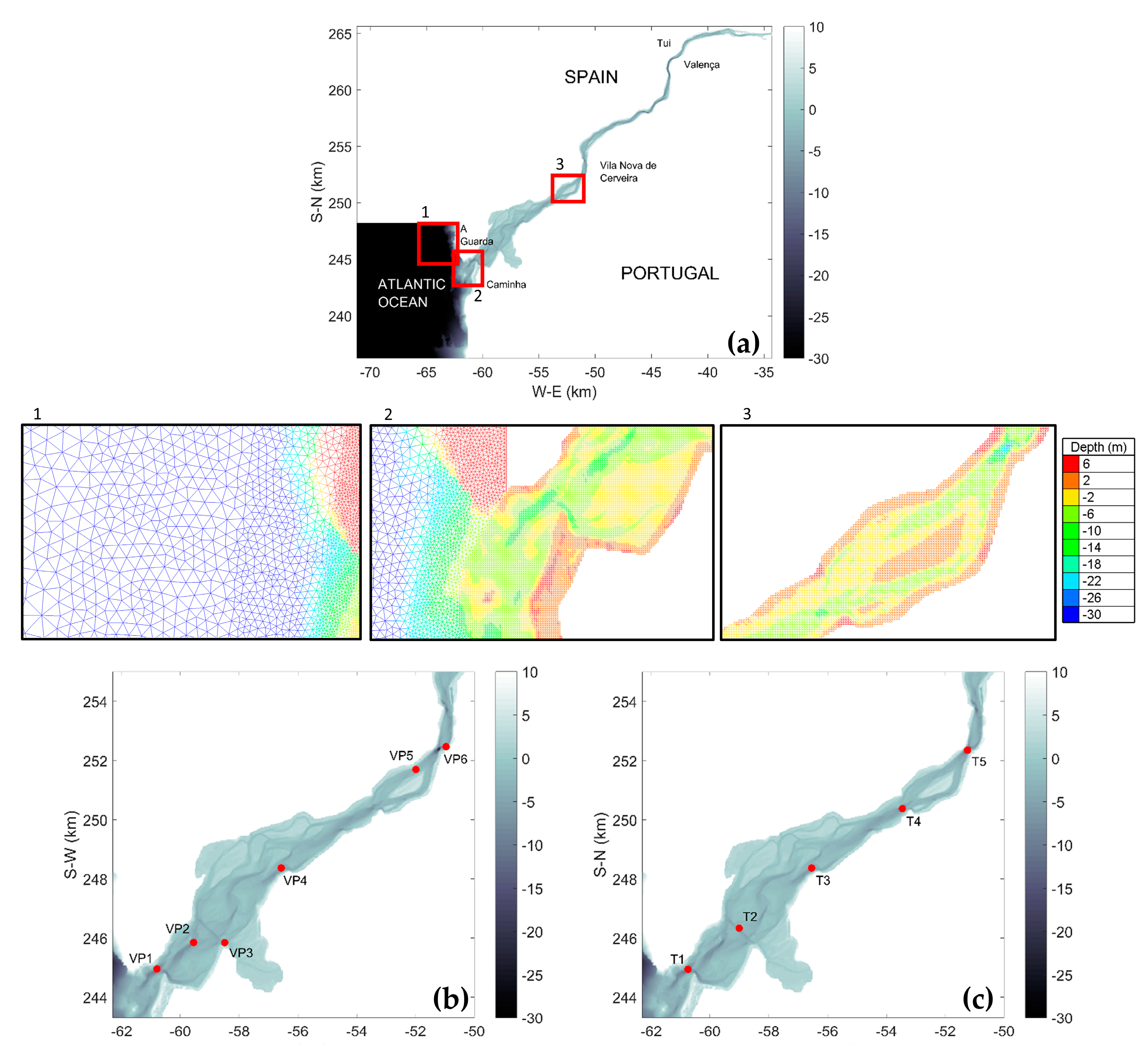
The Minho is an international river that constitutes a natural border between Portugal and Spain in its last 70 km. Being the second most important freshwater source in the northern part of the Western Iberian coast, it flows into the Atlantic Ocean between A Guarda (Spain) and Caminha (Portugal). The estuary is 40 km long, with sections between 200 m (upriver) and 2000 m wide (near the river mouth). At the mouth, the cross-section is narrower, about 300 m wide (see Figure 1a). This is a very shallow estuary, with a mean depth of 4 m [10,11]. However, regions with depths of 11 m or even 20 m can be found near Valença and Vila Nova de Cerveira, respectively, associated with a narrowing of the main channel, reducing the cross-sectional area and increasing river flow velocities (Figure 1a). The estuary presents a semidiurnal high-mesotidal regime, with the tidal range varying between 2 m (during neap tides) and 4 m (in spring tides), and an average residence time of 1.5 days [12]. It is a partially mixed system, where a vertical stratification can be formed when the system generates a salt wedge configuration [13,14]. Associated with this salt wedge, salt intrusion can spread as far as 17 km from the mouth during the highest spring tides [15]. 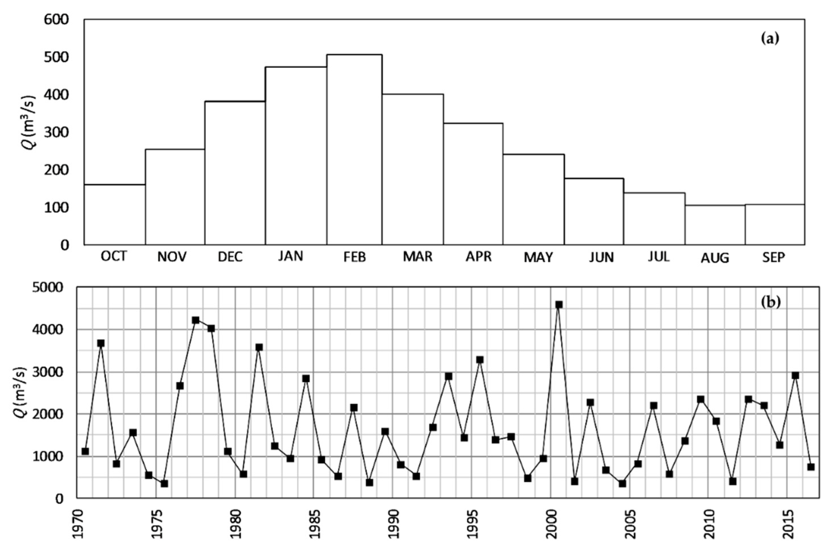Additionally, during spring tides, the effect of the tide can extend up to 40 km upstream due to the tidal regime and the smoothness and low slope of the Minho outlet [13,16,17]. The river flow rate that reaches the estuarine region is mainly controlled by a hydroelectric power plant dam at Frieira (Spain), placed 80 km upstream from the mouth. Downstream from Frieira, the river runs freely through small canyons with a granitic bed. The estuary itself is characterized by a sandy bed where the sediments present a certain homogeneity (medium to very fine sands), with low concentrations of heavy metals and metalloids [4,8,18,19].

The Minho estuary ecosystem has been intensively studied in terms of its hydromorphological characteristics, water quality, populations and pollution [20]. It is considered a low-impacted estuary (low human intervention), often selected as a reference in ecotoxicological studies, and also as an example for the implementation of water directives in other rivers, due to its water quality [9]. The estuary presents a large diversity of habitats, with several threatened, economically and ecologically valuable species, and an important productivity, key for the nursery and feeding of marine species and ecosystem functioning [8,9]. For these reasons, the Minho estuary is protected by Portuguese and Spanish conservation statutes [10], and is included in the LTER (Long-Term Ecosystem Research) Portugal and LTER Europe programmes [15,20] and in the Natura 2000 Network [21,22]. Furthermore its wetlands are registered in the Inventory of Galician Wetlands, and it is classified as a Zona de Protecção Especial para Aves (ZEP) [23], Important Bird Area (IBA) [24] and a CORINE Biotope [25].

Despite the low level of industrialization in the Minho watershed, there are some threats associated with the risks of pollution, flooding, erosion and silting, poor maintenance of the navigation channels, and coastal degradation. These threats can affect environmental quality and can be considered the main risks in this estuarine region [13,19,26]. In terms of anthropic activities, environmental pressures and impacts have been increasing. The estuary is vulnerable to pollutants due to the long residence time that prevents water from rapidly reaching the ocean, and due to the small estuarine area and the relatively low water volumes that decrease the capacity to dilute contaminants [9].

The main problem of this estuary is the silting. The area above the hydrographic zero (HZ, the level of the lowest astronomical tide, which is 2 m below the local mean sea level) in the central and lower parts of the estuary (between the river mouth and 14 km upstream) represents about 70% of the total area, indicating a high degree of sedimentation. This siltation could be related with high sediment deposition and low river discharge, but also with flow rate regularization and the reduction of the frequency and intensity of floods [27,28]. In this estuarine region, the main physical, hydrological and morphological alterations are related with dam construction, river flow regulation and the development of facilities to support human activities in the estuary [20]. Balsinha et al. [4] remarked that the sediment imbalance observed in the Minho estuary can be due to the influence of Spanish hydroelectric exploitation (dams). Due to this imbalance and silting problems, the navigation channel has to be maintained through dredging, causing impacts in the morphological evolution of the estuary and adjacent coastal areas, as well as impacts on the area’s ecosystems.

The morphodynamic patterns generated by silting produced several constraints to navigation, such as strangulation or rapid variations in bathymetry, and various sandbars that emerge during low tide [11,29]. In addition, some sedimentary islands are present. The largest of these is the Boega Island, located downstream from Vila Nova de Cerveira. During the low water period of spring tides, the connection between the estuary and the sea is restricted to two shallow channels, excavated in the river bottom, with depths of less than 2 m and 1 m (referred to the HZ) for the northern and southern channels, respectively [16,17].

Despite this characterization found in the literature, the dynamics of the Minho estuary is essentially unknown [30] and there is a lack of publications on numerical modelling for this estuary. In Sousa et al. [14] and Pereira [3], numerical models were used to study the interaction of the Minho River with the Galician rias and with the Lima estuary, respectively, yet no detailed analysis of the hydrodynamics of the estuary was performed. Delgado [31] and Portela [28] built numerical modelling tools for the Minho estuary, focusing only on the estuarine sediment transport for a few theoretical scenarios.

3. Methods

3.1. Numerical Model

To simulate the Minho estuary hydrodynamics, the 2DH depth averaged version of the openTELEMAC-MASCARET modelling software was selected, given its capacity to accurately simulate hydrodynamic behaviour in coastal, river and estuarine systems [32]. This modelling tool takes into account the effects of flood/ebb cycles, bathymetry, river discharge, water levels, currents velocity and Coriolis force [33,34,35], allowing the assessment of the flood risk of a region [6,36]. The numerical model suit solves the shallow water equations, considering several processes, such as turbulence, bed friction, supercritical and subcritical flows, as well as density effects due to horizontal temperature and salinity gradients. Despite the complexity of the parameters involved in estuarine systems, 2DH models are able to produce accurate solutions with good agreement between measured and simulated hydrodynamic data. The works of Horrit and Bates [36], Hu et al. [37], Néelz and Pender [38,39], Robins and Davies [34], Monteiro et al. [35], Wan et al. [40], Symonds et al. [41] and Iglesias et al. [6] demonstrate that 2DH models are capable of adequately predicting velocity, flood extent and water level, proving that 2DH models results are suited for risk assessment. 2DH models are widely used by the scientific community to represent the hydrodynamics of shallow estuarine systems, reinforcing their applicability for the Minho estuary region [14,42,43].

Telemac2D was implemented using a finite element method solver for numerical discretization and integration, where the continuity equation is replaced by a wave equation [44]. An unstructured linear triangular mesh was constructed using several topographic and bathymetric datasets. The topographic data was provided by the Portuguese Direção Geral do Território [45] as a 1-m resolution Digital Terrain Model (DTM). This DTM is based on a nation-wide altimetric survey carried on in 2011 with a LiDAR (Light Detection And Ranging). The bathymetric data for the estuarine region and the adjacent coastal area was provided by the Portuguese Instituto Hidrográfico (IH) [46]. It was obtained in 2006 and presents a resolution of 30 m inside the estuary and 50 m in the adjacent coastal region. Additional ocean bathymetric data was extracted from the GEBCO database [47], with a 300-m resolution. The different data sets were interpolated to a single finite element mesh, using a kriging algorithm [48,49]. The mesh covers the estuarine region from the river mouth up to 27 km upstream, and an adjacent coastal area up to 9 km offshore and an extension of 12 km in north-south direction (Figure 1a), and has 108,748 elements and 56,387 nodes. The resolution of the mesh varies from about 400 m at the ocean boundary to 30 m inside the estuarine region. Land areas were considered as wet-dry zones.

During the simulations, the time-step was set to 6 s to guarantee numerical stability. Bottom friction was included considering a Chézy friction law. Friction and eddy diffusivity coefficients were obtained after calibration processes and sensitivity testing. Horizontal eddy viscosity and diffusivity coefficients of 1 m²∙s⁻¹ and a Chézy friction coefficient of 53 m^1/2·s⁻¹ were imposed in the entire domain. A constant Coriolis factor of 9.5 × 10⁻⁵ s⁻¹ was included, using the mean latitude value for the computational domain. A spin up period of 6 h was considered at the beginning of each simulation to prevent any spurious oscillation. This spin up period included a ramp for both tide level and river flow rate. Salinity and temperature values for the open boundaries, considering winter conditions, were extracted from available literature [10,13,15,17,50,51,52]. Salinity was set to 0 PSU for the river boundary and 35.8 PSU for the ocean boundary. Water temperature was set to 8 °C for the river boundary and 17 °C for the ocean boundary. Time series for the ocean tide level were obtained from the TPXO.2 tidal model [53]. Finally, hourly and daily mean river flow rates were provided by the Spanish Confederación Hidrográfica Miño-Sil (CHMiñoSil) [54], to force the numerical simulations at the river boundary. Hourly mean values since 1 January 2008 were provided at Salvaterra do Miño, a location 40 km upstream from the estuarine mouth, while daily mean values were available since 1 October 1970 at the last dam at Frieira, located 80 km upstream from the estuary mouth.

3.2. Field Data

Between 2005 and 2007 several in situ campaigns were performed in the Minho estuary under the ECOIS—Estuarine Contributions to Inner Shelf dynamics project [4,11,55]. For this study, data on currents and water elevation were selected at five estuarine stations (VP1–VP4 and VP6). Characteristics and positions for these stations are given in Figure 1b and

Table 1. Characteristics of the validation points.

Station	X (m) 1	Y (m) 1	Time (year)	Data Type
VP1	−60,795.140	244,954.440	2006	Velocity (fixed depth)
				Velocity (profiler)
VP2	−59,549.860	245,850.170	2006	Velocity (fixed depth)
VP3	−58,495.223	245,847.703	2006	Water level
VP4	−56,569.300	248,367.870	2006	Water level
				Velocity (fixed depth)
				Velocity (profiler)
VP5	−51,985.223	251,697.703	2012–2013	Water level
VP6	−50,961.530	252,475.480	2006	Water level

¹ Horizontal coordinates in datum PT-TM06/ETRS89.

. Hourly water levels at station VP5 were provided by CHMiñoSil [54]. Current velocity measurements were obtained using two different setups: (i) at a fixed depth of the vertical column; and (ii) for the entire water column using current profilers recording velocity data.

3.3. Statistical Evaluation

The accuracy of the numerical results, when compared to the field measurements, was measured using the most common statistical coefficients: the Pearson correlation coefficient:

$$\mathrm{PCC}=\frac{{{\displaystyle \sum }}_{i=1}^N\left(X_p\left(t_i\right)-\overline{X_p}\right)\left(X_m\left(t_i\right)-\overline{X_m}\right)}{\sqrt{{{\displaystyle \sum }}_{i=1}^N\left(X_p\left(t_i\right)-\overline{X_p}\right)}\sqrt{{{\displaystyle \sum }}_{i=1}^N\left(X_m\left(t_i\right)-\overline{X_m}\right)}}$$

(1)

the bias function:

$$\mathrm{Bias}=\frac{{{\displaystyle \sum }}_{i=1}^N\left(X_p\left(t_i\right)-X_m\left(t_i\right)\right)}{N}$$

(2)

the root mean square error (RMSE):

$$\mathrm{RMSE}=\sqrt{\frac{1}{N}{\displaystyle \sum }_{i=1}^N{\left(X_m\left(t_i\right)-X_p\left(t_i\right)\right)}^2}$$

(3)

and the predictive skill:

$$\mathrm{Skill}=1-\frac{{{\displaystyle \sum }}_{i=1}^N{\left|X_p\left(t_i\right)-X_m\left(t_i\right)\right|}^2}{{{\displaystyle \sum }}_{i=1}^N{\left(\left|X_p\left(t_i\right)-\overline{X_m}\right|+\left|X_m\left(t_i\right)-\overline{X_m}\right|\right)}^2}$$

(4)

where N is the number of observations, X_p and X_m the predicted (p) and measured (m) values of variable X for the observation t_i, and $\overline{X(·)}$ is the time average of a distribution.

PCC measures the linear association between the measured and the predicted variables. Its values are between +1 and −1, indicating a total positive or negative correlation, and if PCC = 0, no linear correlation is presented. The bias function provides the difference between the predicted and the measured variable. The values of the bias function are between 0 (or unbiased) and 1. Better comparisons are obtained when the bias function is next to 0. RMSE also estimates the difference between predicted and measured variables. RMSE values are non-negative. RMSE = 0 indicates a perfect fit to the data. Finally, a predictive skill of 1 indicates a perfect agreement between the predicted and the measured data, meanwhile a predictive skill of 0 indicates a complete disagreement [6,56,57,58].

The maximum observed difference and the mean difference between measured and modelled variables were also calculated. Note that for the comparison with the 2DH numerical solutions, the mean vertical velocity was calculated for the current profilers data.

3.4. Modelling Scenarios

For this study, three different hindcasting scenarios, S1, S2 and S3, were considered (

Table 2. Modelling scenarios.

	S1	S2	S3
Time	20 February–9 March 2006	1–13 December 2012	16–26 January 2013
Tide level	TPXO.2	TPXO.2	TPXO.2
River flow (m3 s−1)	Daily mean	Hourly mean	Hourly mean
Run length (days)	18	13	11

). Scenario S1 was run for the period 20 February–9 March 2006, and was used for calibration and validation of the numerical model. Bottom friction and eddy viscosity coefficients were calibrated using water level and velocity data collected at stations VP1 to VP4 and VP6. Due to the lack of hourly mean values for river flow rate before 2008, the simulation was forced with the daily mean values of river flow.

The S2 and S3 scenarios were used also for the validation of the model. Scenario S2 was run for the period 1–13 December 2012, and corresponds to low river flow (LF) conditions. Scenario S3 was run for the period 16–26 January 2013, during conditions of high river flow (HF), i.e., flood conditions, and medium river flow (MF). Water data recorded at station VP5 was used for the validation process. The availability of hourly mean flow rate values to force the river allowed a more accurate representation of the estuarine hydrodynamic patterns.

4. Results

4.1. River Flow Regimes

A database of the mean daily flow rate of the river Minho at the Frieira dam, 80 km from the river mouth, was provided by CHMiñoSil [54]. This database covers a 47 year-long period (1970–2017), which allows a statistical analysis of the flow distribution of the Minho River.

The river presents an annual average flow rate of 272 m³∙s⁻¹, with an important inter-annual variability. The seasonal river flow regime presents a normal behaviour for its latitude (Figure 2a), related with the annual precipitation variability [59]. Maximum flow rates occur during winter and spring (December–April) and the minimum flow rates during an extended summer period (June–October). The maximum annual flow rate mostly occurred in December (12 events), January (10 events) and February (11 events), for the 47-year period covered by the data.

In addition to the seasonal behaviour, there are important differences between dry and wet years, revealing a strong inter-annual variability (Figure 2b). Average flow values above 4000 m³∙s⁻¹ were recorded during extreme flow events in 1978, 1979, 2000 and 2001. If we assume that the probability distribution for extreme flow events follows a Gumbel law [60], this value corresponds to the 20 year return period. Flow rates for some significant return periods are provided in

Table 3. Return periods and river flow.

Return Period (years)	River Flow (m3·s−1)
2	1644
20	3944
100	5383
500	6809

.

4.2. Model Validation

Numerical series for water level and current velocity were extracted at stations VP1–VP4 and VP6, and used to calibrate and validate the model’s physical parameters through comparison with field measurements, for scenario S1 (Table 2). The best error metric results were obtained for a Chèzy friction coefficient of 53 m^1/2∙s⁻¹, and constant horizontal eddy viscosity and diffusivity coefficients of 1 m²·s⁻¹ each.

Keep in mind that the difference between the physical and the numerical flow rates increases with distance from the upstream boundary as no mass input was considered from the river watershed downstream from Frieira. Nevertheless, the Minho tributaries in the estuarine region are minor, presenting very low river flows and small hydrographic basins [54,61]. Therefore, the main flow in the estuarine region will be determined at Frieira.

Numerical outputs for the water levels at stations VP3, VP4 and VP6 match the field measurements relatively well (Figure 3). Only at station VP6 a difference can be noticed during the spring tide. Being located at a narrow section of the river, station VP6 is prone to a higher error in the water level due to an underestimation of the river flow rate. This underestimation can also be caused by the proximity of the station to the riverbank or by some bathymetric mismatch between the real and the modelled configuration at point VP6. Nevertheless, the accuracy of the numerical solution at the calibration points is quite good, as revealed by the small RMSE, the close to null bias and the close to unit correlation and skill coefficients (

Table 4. Error metrics for the water elevation.

Station	r	RMSE (m)	Bias (m)	Skill	Max. Diff (m)	Mean Diff (m)
VP3	0.9635	0.1842	−0.0109	0.9811	0.57	0.12
VP4	0.9238	0.2507	0.0033	0.9606	0.62	0.18
VP6	0.9543	0.1762	−0.0422	0.9635	0.66	0.13

). The maximum differences between measured and modelled water elevations were between 0.57 m for VP3 and 0.66 m for VP6, whereas the mean differences were between 0.12 m for VP3 and 0.18 m for VP4 for the simulated period.

The comparison between current velocity field measurements and numerical solutions is shown in Figure 4 for fixed depth measurements, and in Figure 5 for water column averaged horizontal velocities. The error metrics (

Table 5. Error metrics for the current velocities measured at fixed depth points.

Station		r	RMSE (m·s−1)	Bias (m·s−1)	Skill
VP1	—	0.9200	0.2816	−0.1439	0.9350
VP2	Spring tide	0.9756	0.1607	−0.0642	0.9760
VP2	Neap tide	0.8319	0.1430	−0.0827	0.8663
VP4	—	0.8915	0.2311	−0.1177	0.8799

and

Table 6. Error metrics for the current velocities measured in the entire water column.

Station	r	RMSE (m·s−1)	Bias (m·s−1)	Skill
VP1	0.9536	0.1154	0.0302	0.9718
VP4	0.8444	0.1477	−0.0311	0.8620

) show small RMSE, close to null bias values and to unit correlation and skill coefficients. The behaviour of the modelled currents is quite similar to that of the field-recorded ones. Some differences can be observed in Figure 4. However, a comparison of current velocities should be performed with care. The implemented models are 2DH, therefore, only depth averaged current velocities should be compared. Additionally, fixed depth-recorded velocities are affected by turbulence while numerical velocities are time-averaged in the sense of Reynolds averaging. Nevertheless, as the mean estuarine region is relatively shallow, the current velocity obtained at a fixed depth in the vertical column should be relatively close to the vertical mean value, although larger differences can be expected when the measuring point is within or close to a boundary layer (either the bottom or a side boundary layer). The difference between the numerical and the field-recorded velocities seem to become larger during the neap tides, with the numerical model overestimating the ebb current velocity (Figure 4a,d). Current velocity comparisons presented in Figure 5 revealed a good agreement between the measured vertical averaged velocity and the model solutions, with the best results obtained for station VP1 (Figure 5b and Table 6). At station VP4 (Figure 5b), a time lag in the change of the tide direction seems to appear in the represented tide cycles. However, the number of measurements is too small to confirm this lag, which can also be related with the station’s proximity to the estuarine margin and with differences between the real river flow and the daily mean river flow values considered for the modelled scenario S1.

Finally, a comparison is made for the water level registered at station VP5, for simulations S2 and S3 (Table 2) that were forced with hourly river flow and included low, medium and high flow values. The results are depicted in Figure 6, with error metrics shown in

Table 7. Error metrics for the water level at station VP5 for scenarios S2 and S3.

Scenario		r	RMSE (m)	Bias (m)	Skill
S2	LF	0.9141	0.2049	0.0773	0.9325
S3	MF	0.9806	0.0520	−0.0082	0.9890
S3	HF	0.9859	0.1219	0.0109	0.9924

. A good agreement was found between the simulations and the measurements, expressed by small RMSE, close to null bias values and close to unity correlation and skill coefficients.

Compared with results from previous works developed for the Minho and even for other estuaries [3,6,34,42,43,62,63,64], the here presented validation results show a similar or even better accuracy. This highlights the ability of Telemac2D to accurately reproduce the estuarine hydrodynamics of the Minho region.

4.3. Tide Propagation

Water elevation values were extracted for non-flooding (S2) and flooding (S3) scenarios for five stations across the estuarine region (Figure 1c). Stations from T1 (downstream) to T5 (upstream) were selected as being deep enough to allow the vertical development of the tide (

Table 8. Depth (in metres referred to the MSL) of the considered numerical tidal gauges and distance to the ocean (km).

Tidal Gauge	Depth (m)	Distance to the Ocean (km)
T1	9.1	0
T2	2.3	2
T3	6.2	5.5
T4	7.1	9.5
T5	20.4	12

).

The results revealed a small delay in the tide phase from T1–T5, with an asymmetry of the tide curve that increases upstream (see Figure 7 and Figure 8). The tidal range is larger at T1, close to the oceanic boundary. As we move upriver, the tidal range diminishes associated with a diminution of the low tide semi-amplitude, which produces an increase of the mean water level in this direction. The semi-amplitude corresponding to low tide does not develop completely, which is more noticeable at T5, the most upstream station.

This asymmetry is more noticeable for the non-flood conditions modelled in Scenario S2 (Figure 7) and can also be represented by the tide phase lag between the several considered stations (from T1 to T5) (

Table 9. Mean modelled tide phase differences. HT: high tide; LT: low tide.

	T1 vs. T2		T1 vs. T3		T1 vs. T4		T1 vs. T5
	HT	LT	HT	LT	HT	LT	HT	LT
S2 mean tide phase difference
min	8.75	33.75	21.25	103.33	35.41	136.25	56.25	162.5
h	0.15	0.56	0.35	1.72	0.59	2.27	0.94	2.71
S3 mean tide phase difference
min	9.5	28	22	72.5	34.5	102.5	65	114.45
h	0.16	0.47	0.37	1.21	0.57	1.71	1.08	1.91

). Analysing the S2 results, a small delay can be observed when the mean lag for the high tide propagation is represented, revealing time differences for reaching the high tide values between 9 min (T1 vs. T2 stations) and 56 min (T1 vs. T5 stations). Calculation of the mean lag for the low tide shows differences between 34 min (T1 vs. T2 stations) and 162 min, which is close to 3 h (T1 vs. T5 stations). This asymmetry is smaller for the S3 scenario due to the high river flow considered (Table 9). For flooding conditions, the surface elevation away from the river mouth is strongly dependent on the river flow rate, and a tidal range of 2 m at station T1 becomes a 0.5 m tidal range at station T5 (Figure 8). Nevertheless, and despite the extreme flood event depicted in S3 (3000 m³·s⁻¹), the tide still has an effect on the water elevation. This is observed even at the most upstream station, T5, with some sinusoidal behaviour but with less amplitude than at T1. The strong flow also reduced the tide amplitude even at T1, but its effect in the water elevation is still noticeable, revealing that this estuary is tide-dominated. The obtained results are in agreement with Zacarias [29], who also observed this effect analysing in situ data.

The asymmetry of the tide can be described as the distortion of the dominant lunar semi-diurnal M₂ tide component by the higher-frequency overtides [65]. The most important harmonic overtide responsible for the distortion of the tidal wave and for tidal asymmetry in coastal regions is the M₄ constituent [66]. Amplitude and phases of these two tidal constituents can be used to describe the tide effects inside estuarine regions. Following Friedrichs and Aubey [67], Seim et al. [68], Dias and Sousa [69] and Moore et al. [66], the tidal distortion factor and the tidal dominance factor can be calculated using the constituents’ amplitudes (amp) and phases (θ), respectively. If M_4amp/M_2amp > 0.01, a significant distortion of the tidal wave should be expected, and if 2M_2θ − M_4θ present values between 0° and 180°, the system will be flood-dominated, otherwise, it will be ebb-dominated.

The M₂ and M₄ amplitudes and phases were calculated performing a harmonic analysis of astronomical tidal constituents, considering the water level extracted at T1 to T5 stations for the S2 and S3 scenarios. To perform this analysis, the T_TIDE tool was chosen [70]. The obtained results (

Table 10. Tidal amplitude (amp) and phase (θ) of the M₂ and M₄ tidal constituents and tidal distortion and tidal dominance factors for T1 to T5 stations during S2 and S3 scenario simulations.

Scenario	Station	M2		M4		Tidal Distortion	Tidal Dominance
		Amp (m)	θ (°)	Amp (m)	θ (°)
S2	T1	0.908	73	0.028	98	0.031	49
	T2	0.835	81	0.046	96	0.055	66
	T3	0.632	93	0.094	128	0.149	58
	T4	0.559	101	0.084	137	0.151	65
	T5	0.415	113	0.054	172	0.129	54
S3	T1	0.753	92	0.012	125	0.015	58
	T2	0.676	99	0.024	113	0.036	85
	T3	0.495	106	0.042	173	0.085	40
	T4	0.366	112	0.039	211	0.107	12
	T5	0.205	114	0.046	257	0.224	28

) show a diminution in the amplitude and phase of the M₂ constituent in the upstream direction for both scenarios, which suggest the absence of resonance modes in this estuary [71,72]. The M₄ constituent amplitude increases between T1 and T3 and diminishes between T3 and T5, while its phase increases upstream for both scenarios. Tidal distortion and tidal dominance factors (Table 9) confirm that the Minho estuary it is a flood dominated estuary, where a considerable distortion of the tidal wave can be expected in the entire region, being more distorted at the upstream locations (T3 to T5).

4.4. Current Patterns

The analysis of the current patterns revealed several configurations of the Minho estuary depending on the imposed river flow and tide. Figure 9 presents the velocity for several selected simulation time-steps for the Scenario S3, particularly the ones that describe the estuary state during HF and rising tide near the high tide (RT-HT; Figure 9a), MF and RT-HT (Figure 9b) and MF and falling tide near the low tide (FT-LT; Figure 9c). Higher velocities are obtained for this scenario when HF (~3000 m³·s⁻¹) conditions are imposed (Figure 9a). These strong velocities are present even during RT-HT conditions. Despite the strong river flow imposed at the upstream boundary, the widening of the estuarine area near the mouth reduces velocity values, by distributing the flow energy across a wider area. It was also observed that the HT value (0.8 m) simulated during HF conditions is not large enough to reverse the river flow to an upstream direction at the estuary mouth, as downstream velocities are obtained for the entire estuarine region. When compared with other S2 and S3 simulation time-steps (Figure 9b,c, and Figure 10), Figure 9a shows large regions of the estuarine margins, the northern part of the Boega Island and several sand bars in the northern estuarine margin that are flooded, and the water masses present velocities varying from 0.1 m·s⁻¹ to 1 m·s⁻¹. The effects of floods in the margins are buffered by the large estuarine area and by the presence of wetlands minimising the risk for human settlements. Nevertheless, the flooding patterns can change the morphology of the wetlands, altering the ecosystem properties in this region.

Patterns similar to those represented in Figure 9a,b, for flow rates close to 3000 m³·s⁻¹, and 1000 m³·s⁻¹, respectively, were obtained by Delgado et al. [27] for a 2500 m³·s⁻¹ flow rate. The tide conditions represented in Figure 9b (+1 m) are not able to reverse the downstream currents in the estuarine mouth. Nevertheless, the velocity values are smaller in this area than the ones obtained in Figure 9a for HF conditions. Despite the tide not being able to induce the inversion of the flow direction, even at the mouth (Figure 9b), it diminishes the currents velocity in the entire estuarine area. In comparison, stronger current velocities are obtained for FT-LT conditions for the entire estuarine area, as shown by the velocity patterns in Figure 9c for a flow rate of 1000 m³·s⁻¹ and FT-LT (−1.1 m) conditions. This means that a sub-critical flow is developed, also demonstrated by values smaller than one of the Froude number (Fr) in the entire area (not shown). The downstream boundary (the water level at the ocean) affects the flow upstream, inhibiting the complete development of the velocities in the wider part of the estuarine area. Even for strong river flows, the tide has a significant effect in this estuarine region, as was also demonstrated in the previous section.

When LF conditions are simulated (see Figure 10), it can be seen that the tide is able to reverse the currents at the mouth (Figure 10a), even if the river flow is near the mean river flow for the winter season (450 m³·s⁻¹). The simulated tide, representing spring tide conditions (+1.6 m), produces an upstream movement of the water masses between the river mouth and the downward part of the Boega Island. This movement is related with sub-critical flow conditions (Fr < 1 in the entire estuarine region, not shown) and with the higher water levels at the ocean side rather than at the river side of the estuary. The two river branches that surround the island present very low or null velocities and, upstream from the island, the currents change to downstream directions. For smaller river flows (~110 m³·s⁻¹) even the smaller tides, as the one considered in the Figure 10b (+0.8 m), are strong enough to reverse the estuarine circulation from the mouth to the upstream limit of the estuarine region considered in this study. Nevertheless, and if LF and FT-LT conditions during neap tides are represented (Figure 10c), the currents patterns present downstream directions in the entire area, with higher values than those observed for RT-HT conditions (Figure 10b). This is related with the sub-critical flow conditions in the estuary. During neap tides, the HT conditions are not large enough to be higher than the upstream level of the river, and no reverse flow is developed. However, as they are higher than the LT conditions, they force the water level within the estuary to be higher than during LT. Thus, for the same flow rate, the flow velocity is lower for a higher water level. A ramification of the water masses was observed, and the outflow of the estuarine water takes place through several canals at the wider section of the estuary. It is expected that, under these conditions, several estuarine areas become emerged. The obtained velocity values are in agreement with the ones modelled by Portela [28] and Delgado et al. [27] during LF conditions and also with the measured values described by Delgado [31] and obtained by IH [73], Consulmar [74] and CEDEX [75].

5. Discussion

A numerical model was developed for shallow water estuaries to represent the main hydrodynamic patterns and their drivers (river flow, tides and bathymetry). It was applied to one of the most important estuarine regions of the Portuguese coast: the Minho estuary.

The dynamics of shallow areas depends strongly on the tides, and the Minho estuary is no exception. This estuary is tide-dominated rather than river-dominated, which means that tidal currents will transport upstream the bedload sediment, which mainly comes from the sea.

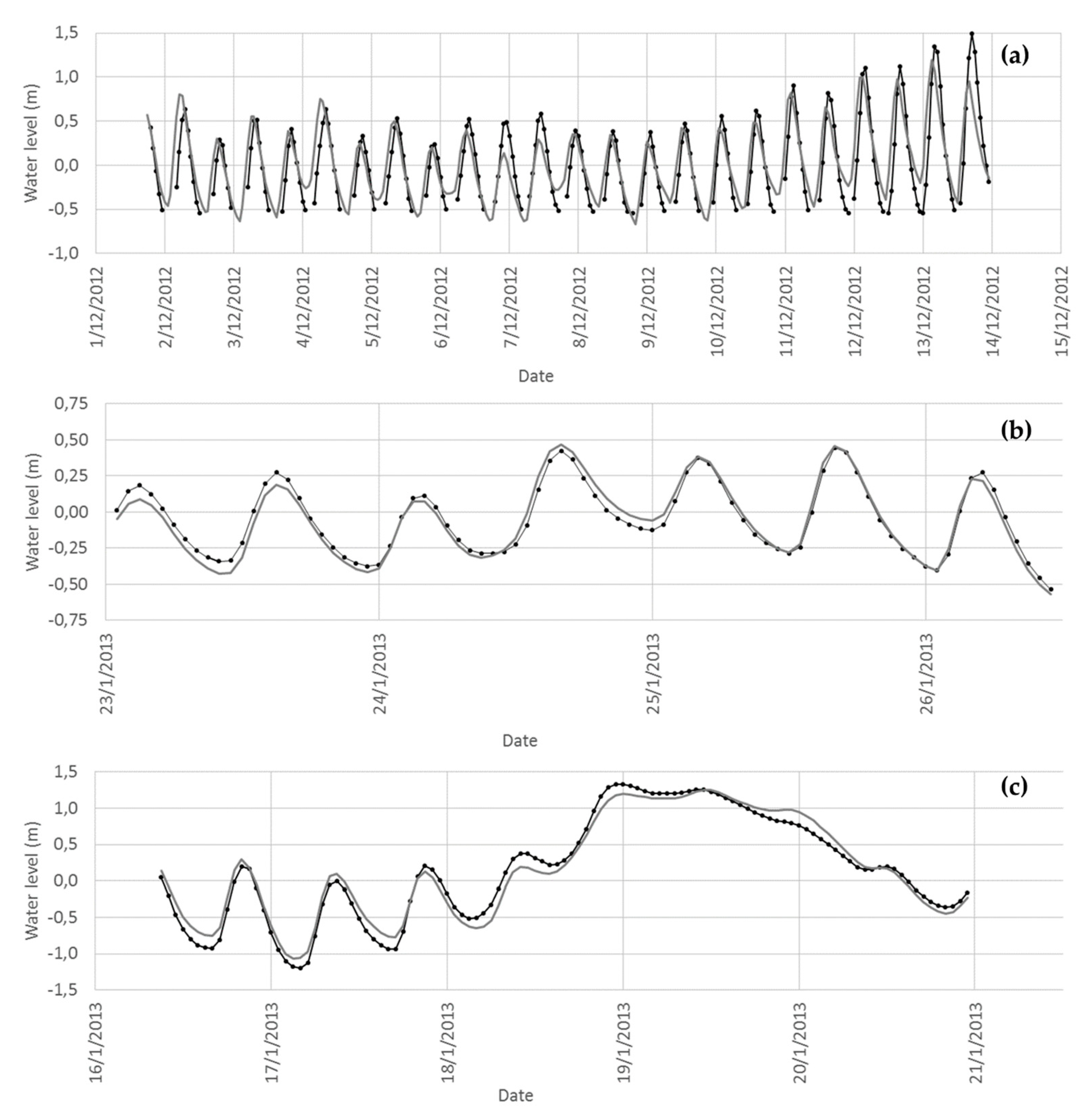
Results show a delay in the tide phase with a marked asymmetry of the tide curve that increases upriver. 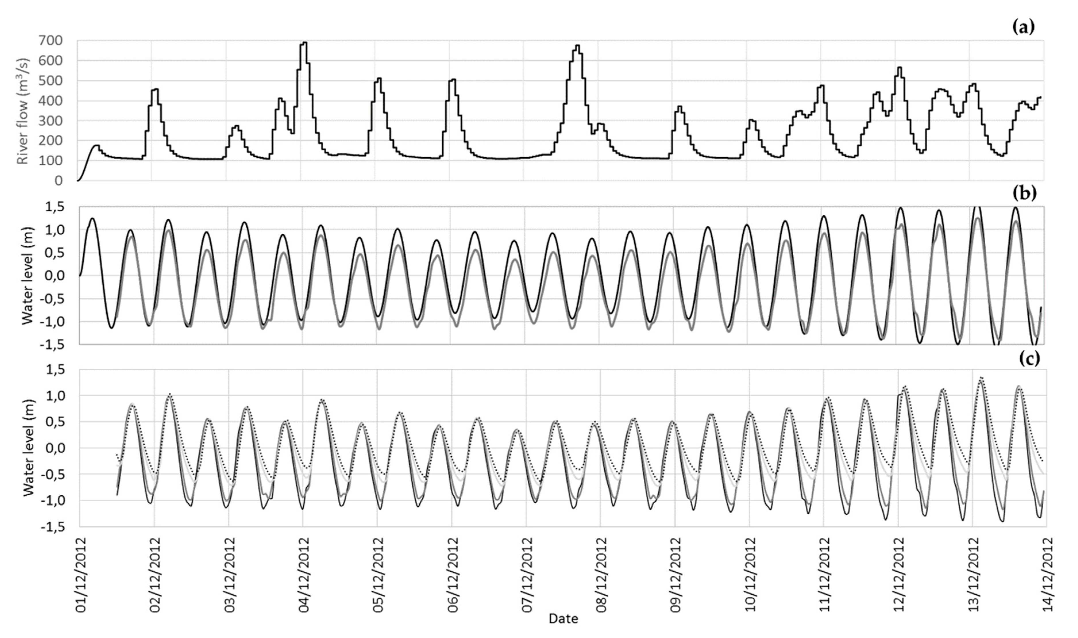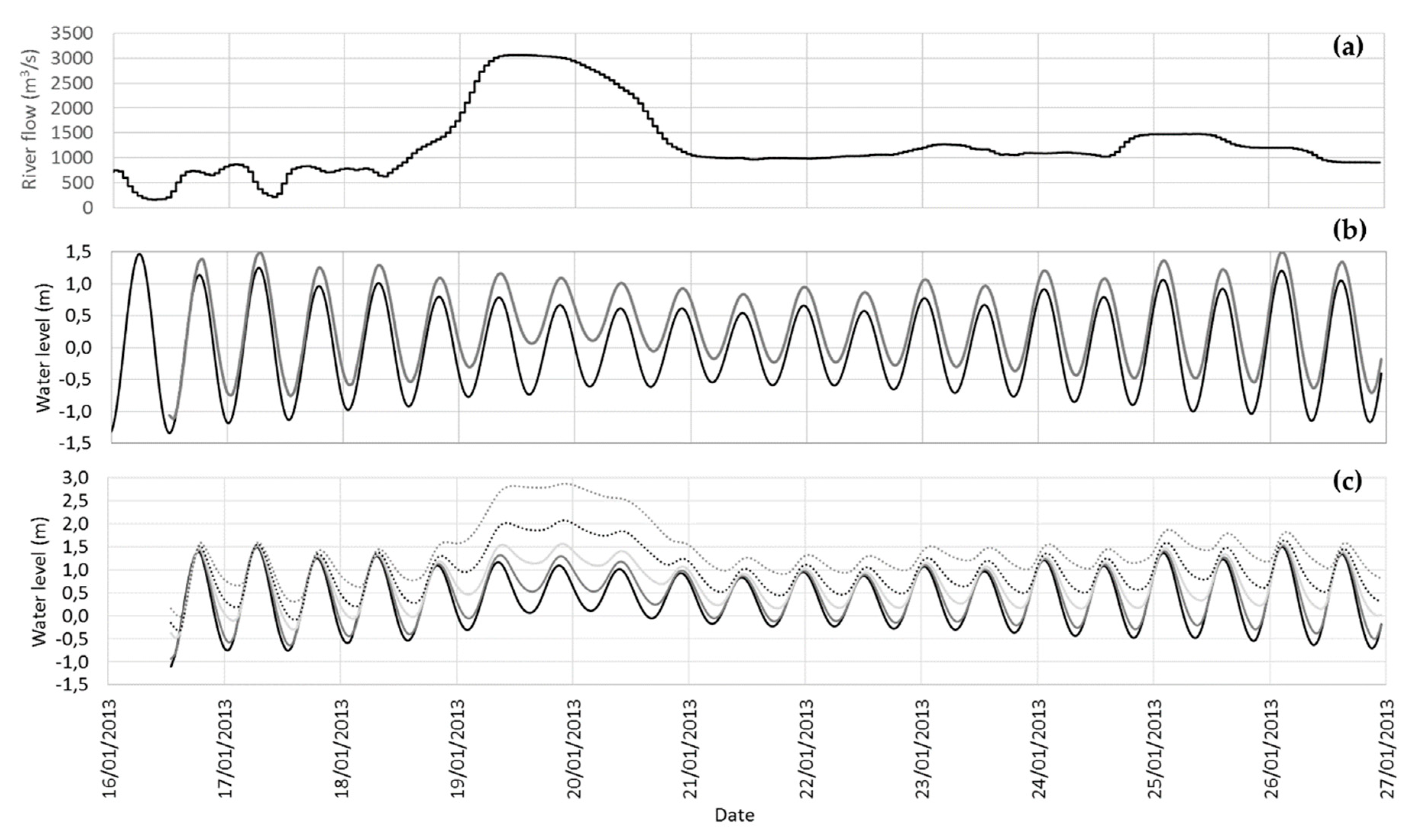Several authors, which also observed this asymmetry with in situ data, suggested that this tide irregularity, related with a non-complete development of the semi-amplitude during low tide events, could be produced by bathymetric constraints and also by the non-linearity caused by energy dissipation associated with friction [11,27,29,31,76]. This asymmetry is more noticeable during non-flood conditions, although the tide still has an effect on the water elevation during strong river flows, but the tidal range is decreased by greater runoff, similar to the results obtained by Uncles et al. [77]. The river flow can reduce the tide amplitude inside the estuarine region but cannot supress its effects, revealing that this estuary is tide-dominated.

The asymmetry of the tide can also be demonstrated using the amplitudes and phases of the M₂ and M₄ tidal harmonic constituents. An upstream diminution of M₂ was observed, suggesting the absence of resonance modes and the presence of tidal flats and shallow waters that slow down the tidal propagation due to frictional energy dissipation and non-linear transfers of energy [71,72]. Normally, in estuarine regions, a reduction of the amplitude of the tides and a phase lag due to the effect of the bottom friction is expected [72]. At the same time, the observed upstream augmentation of M₄ can be related with friction and channel convergence, which transfer energy to the shallow-water tide constituents [68]. The tidal distortion factor revealed a considerable distortion of the tidal wave in the entire estuary, being more distorted at the upstream locations, as was demonstrated when the tide evolution at different estuarine locations was represented. The tidal dominance factor classifies this estuary as flood dominated, in agreement with previous works that show that shallow water estuaries are generally flood dominated [65,66]. In a flood dominated estuary the ebb takes longer than the flood, producing longer lags during low water levels than at high water levels [69], as also observed for the Minho estuary. This analysis reflects the accreting nature of this region, with flood currents producing a net marine sediment transport into the estuary, and reflecting that tidal asymmetry is a controlling factor of the estuarine morphological development [65,66]. Similar results were obtained by Moore et al. [66] for the Dee estuary (UK), where flood dominance is likely to induce net sediment transport into the estuarine region.

It is important to remark that the central problem of the Minho estuary region is siltation. This region presents a large amount of tidal flats. Previous studies indicated that the presence of tidal flats in estuarine regions can point at ebb-dominated estuaries, normally associated with a convexity in the profile of those flats [66,78,79]. Nevertheless, when the tidal flats are connected with an estuarine region where the tide is slowed down due to, for example, bottom friction, the generated asymmetry is of the flood-dominated type due to a reduction of the M₂ amplitude [79]. This is the case of the Minho estuary. This flood dominance will lead to a net transport of fine and coarse sediments into the estuarine region that can also reduce the mean depth and increase the bottom friction effect and the amount of tidal flats.

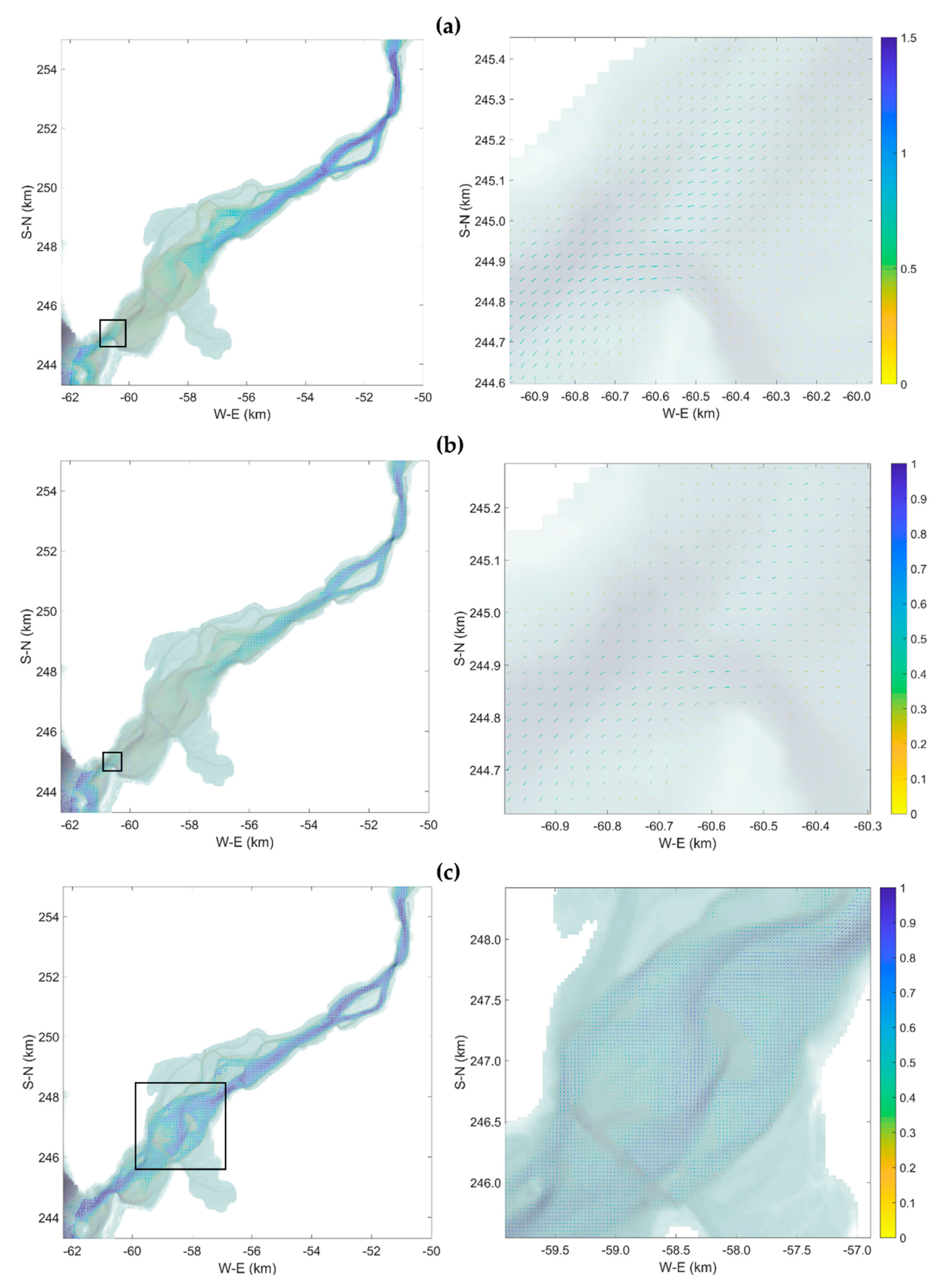
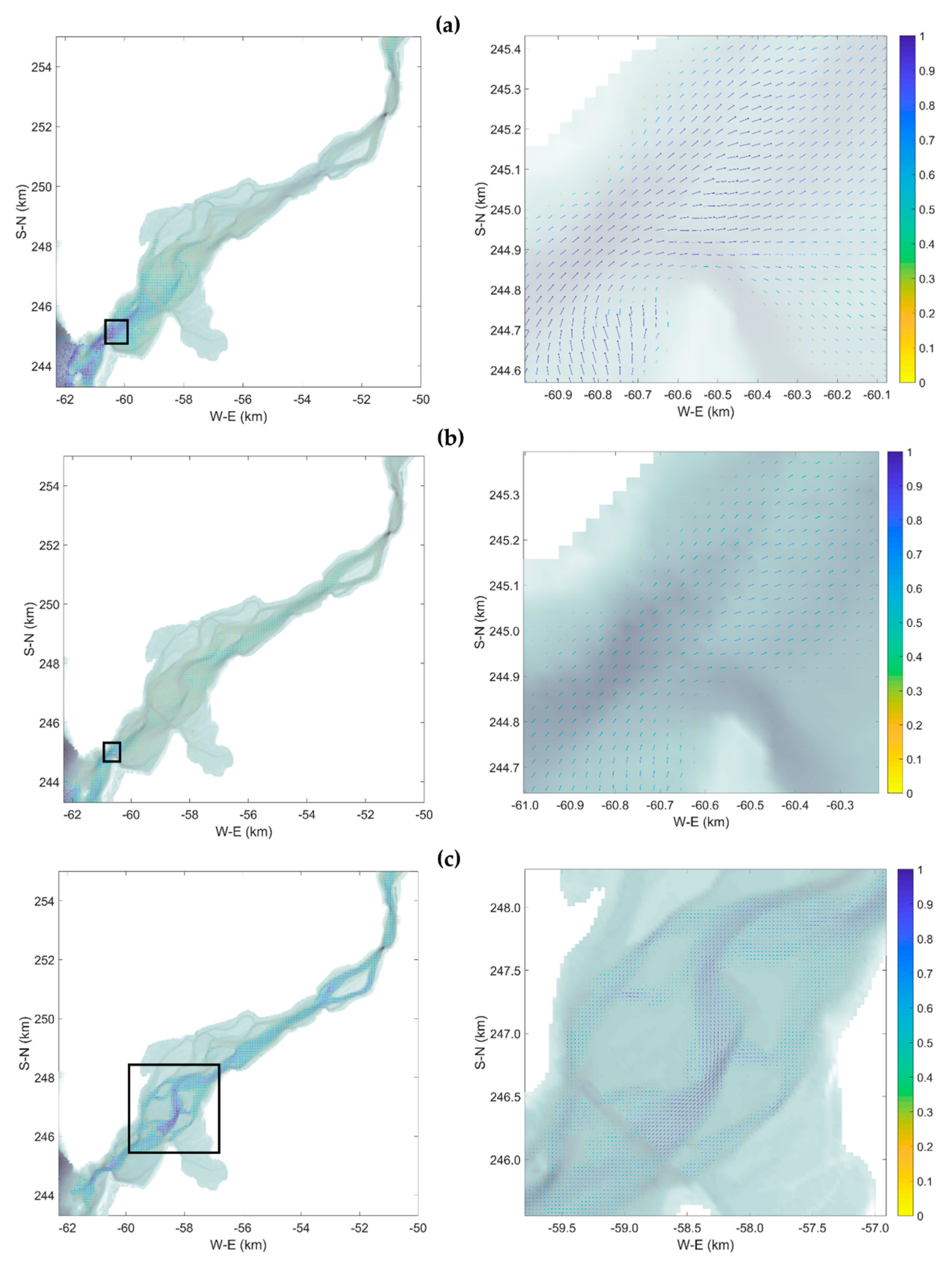
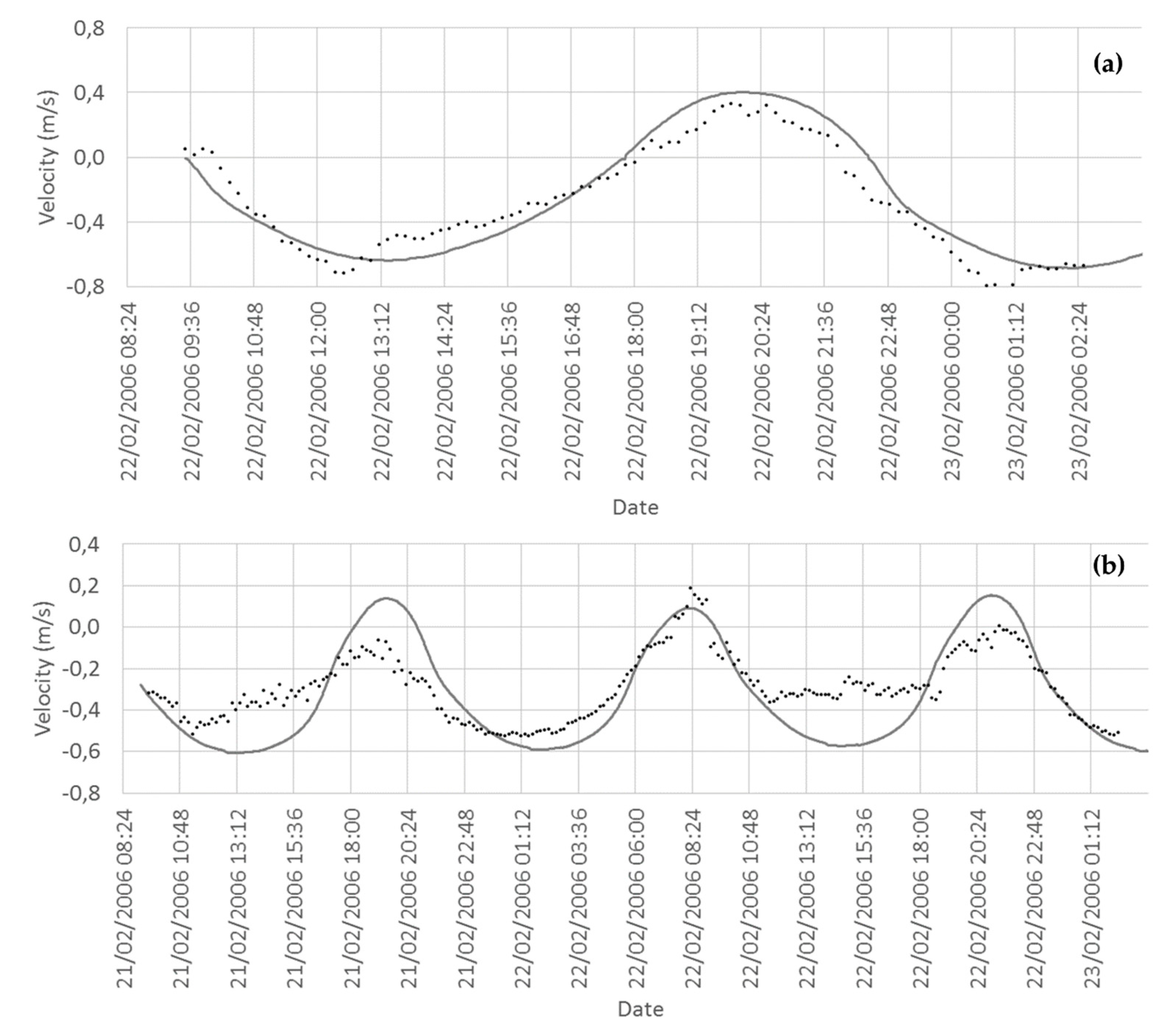
The velocity patterns obtained in this study revealed that the Minho estuary presents current velocities comparable with other national (Portuguese) and international estuarine regions [2,6,34,37,40,64,68,72,79,80]. The currents velocity conditions showed the typical pattern of a semi-diurnal tide, where the ebb tide presents stronger velocities than the flood, because bottom friction increases vertical shear during ebb [80]. The velocity reaches higher values during ebb than flood also due to the imposed river flow conditions, producing a stronger tidal mixing during the ebb [64]. Regarding the estuarine sections, the velocities under normal conditions are stronger in the (narrower) mouth than in the wider section of the estuary. Secondary maximum velocities can be found in the narrower sections upstream. During flood conditions, large parts of the estuary are flooded due to their low topography and their wetlands characteristics. High velocities were obtained in most of the estuary, except in the wider region upstream from the mouth where the widening of the estuary distributes the flow energy.

6. Conclusions

In this work a 2DH numerical model for shallow estuaries based on the openTELEMAC-MASCARET modelling suit was developed and applied to the Minho estuary region with satisfactory results.

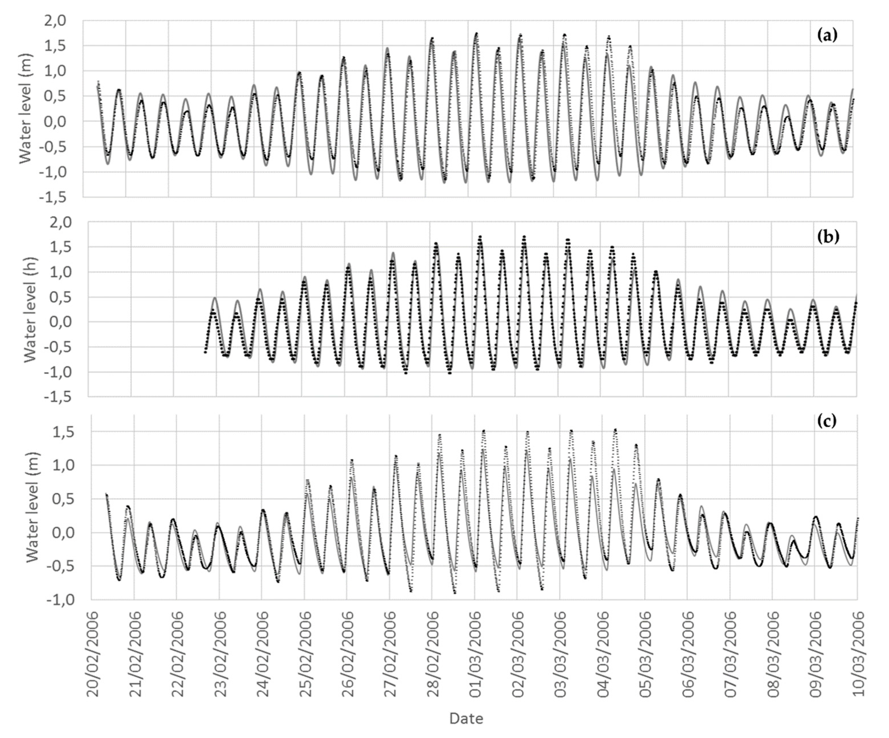
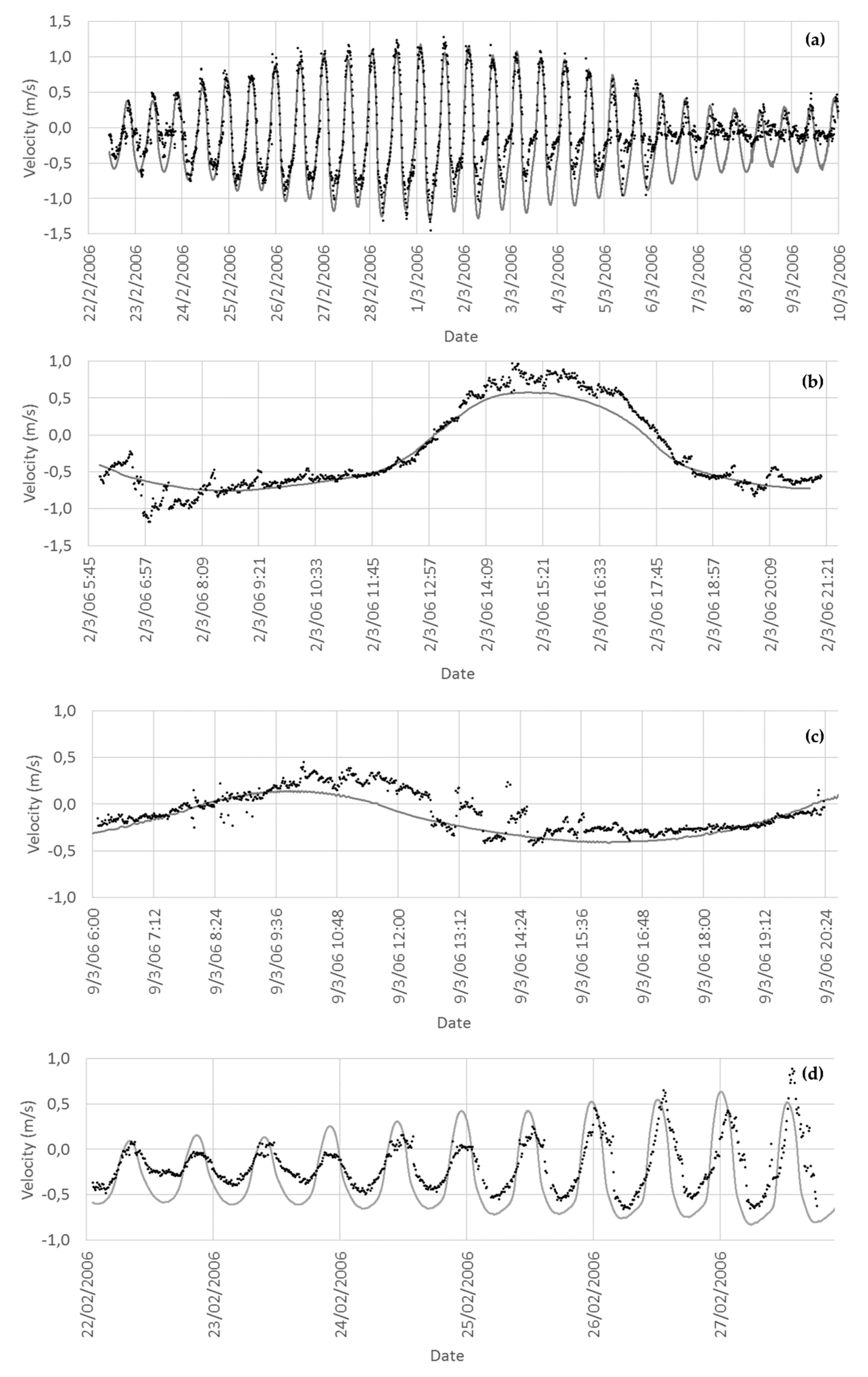
First of all, calibration and validation procedures were performed comparing in situ data and modelling results of water level and current velocity at several estuarine locations. Results revealed a general good agreement for the several considered scenarios, which include high-, medium- and low-flow conditions. Differences in water levels can be explained by the proximity of the measuring station to the riverbank or by some bathymetric mismatch between the real and the modelled configuration. As expected, comparisons between fixed depth measurements and modelled solutions for currents velocities revealed some differences. These differences are reduced and the statistical errors are improved when vertical averaged velocity measurements are selected instead of fixed depth measurements.

The main results are that the Minho is a tide-dominated estuary with a delay in the tide phase and a marked asymmetry in the tide curve that increases upriver. Upstream diminution of M₂ and upstream augmenting M₄ tidal harmonic constituents were observed inside the estuary, suggesting a slowing down of the tidal propagation due to frictional energy dissipation, non-linear transfers of energy and channel convergence.

This estuary also revealed to be flood-dominated, reflecting the net transport of marine sediments into the estuarine region and explaining its siltation problems.

Regarding the velocity patterns, velocities are higher during ebb tide than during flood tide, with stronger velocities in the narrower sections. During flooding events, large estuarine regions are flooded due to their low topography and their wetlands characteristics.

The different scenarios simulated in this study revealed that variations in the intensities of the main driving forces of this estuary—fluvial flow and tide—alter the behaviour of the hydrodynamical patterns within the estuary, being also very dependent on the estuarine bathymetric characteristics, which also define the main flow patterns.

It was demonstrated that the numerical modelling tool implemented for this estuarine region was able to depict and forecast the main regional problems, and can be used as a decision-making support tool for an effective and integrated estuarine management. Future studies will be focused on the representation of climate change effects and human interventions, including effects of pollutants, nutrients and sediment transport, depicting the impacts, adaptation and vulnerability of this estuarine zone and providing valuable information to promote population safety and the sustainability of the Minho estuary ecosystems.

References

1. Costanza, R.; D’Arge, R.; de Groot, R.; Farber, S.; Grasso, M.; Hannon, B.; Limburg, K.; Naeem, S.; O’Neill, R.V.; et al. The value of the world’s ecosystem services and natural capital. Nature 1998, 387, 253–260. [Google Scholar] [CrossRef]
2. Arndt, S.; Lacroix, G.; Gypens, N.; Regnier, P.; Lancelot, C. Nutrient dynamics and phytoplankton development along an estuary-coastal zone continuum: A model study. J. Mar. Syst. 2011, 84, 49–66. [Google Scholar] [CrossRef]
3. Pereira, H. Coupled Modelling of the Minho and Lima Estuaries: Hydrological Response to Climate Changes. Master’s Thesis, Universidade de Aveiro, Aveiro, Portugal, 2016. [Google Scholar]
4. Balsinha, M.J.; Santos, A.I.; Alves, A.M.C.; Oliveira, A.T.C. Textural composition of sediments from Minho and Douro estuaries (Portugal) and its relation with hydrodynamics. J. Coast. Res. 2009, 56, 1330–1334. [Google Scholar]
5. Hopkinson, C.; Vallino, J.J. The relationships among man’s activities in watersheds and estuaries: A model of runoff effects on patterns of estuarine community metabolism. Estuaries 1995, 18, 598–621. [Google Scholar] [CrossRef]
6. Iglesias, I.; Venâncio, S.; Pinho, J.L.; Avilez-Valente, P.; Vieira, J.M.P. Two models solutions for the Douro estuary: Flood risk assessment and breakwater effects. Estuaries Coasts 2018, 42, 348–364. [Google Scholar] [CrossRef]
7. Bastos, L.; Bio, A.; Iglesias, I. The importance of marine observatories and of RAIA in particular. Front. Mar. Sci. 2016, 3, 1–11. [Google Scholar] [CrossRef]
8. Domínguez García, M.D.; Horlings, L.; Swagemakers, P.; Simón Fernández, X. Place branding and endogenous rural development. Departure points for developing an inner brand of the River Minho estuary. Place Brand. Public Dipl. 2013, 9, 124–140. [Google Scholar] [CrossRef] [Green Version]
9. Ribeiro, D.C.; Costa, S.; Guilhermino, L. A framework to assess the vulnerability of estuarine systems for use in ecological risk assessment. Ocean Coast. Manag. 2016, 119, 267–277. [Google Scholar] [CrossRef]
10. Freitas, V.; Costa-Dias, S.; Campos, J.; Bio, A.; Santos, P.; Antunes, C. Patterns in abundance and distribution of juvenile flounder, Platichthys flesus, in Minho estuary (NW Iberian Peninsula). Aquat. Ecol. 2009, 43, 1143–1153. [Google Scholar] [CrossRef]
11. Reis, J.L.; Martinho, S.; Pires-Silva, A.A.; Silva, A.J. Assessing the Influence of the River Discharge on the Minho Estuary Tidal Regime. J. Coast. Res. 2009, 56, 1405–1409. [Google Scholar]
12. Ferreira, J.; Abreu, P.; Bettencourt, A.; Bricker, S.; Marques, J.; Melo, J.; Newton, A.; Nobre, A.; Patricio, J.; Rocha, F.; et al. Monitoring Plan for Portuguese Coastal Waters. Water Quality and Ecology. Development of Guidelines for the Applications of the European Union Water Framework Directive. IMAG-IMAR: Portugal, 2005. Available online: https://www.researchgate.net/publication/276921166_Monitoring_Plan_For_Water_Quality_and_Ecology_for_Portuguese_Transitional_and_Coastal_Waters_Development_of_guidelines_for_the_application_of_the_European_Union_Water_Framework_Directive (accessed on 15 May 2019).
13. Sousa, R.; Guilhermino, L.; Antunes, C. Molluscan fauna in the freshwater tidal area of the River Minho estuary, NW of Iberian Peninsula. Ann. Limnol. Int. J. Limnol. 2005, 41, 141–147. [Google Scholar] [CrossRef] [Green Version]
14. Sousa, M.C.; Vaz, N.; Alvarez, I.; Gomez-Gesteira, M.; Dias, J.M. Modeling the Minho River plume intrusion into the Rias Baixas (NW Iberian Peninsula). Cont. Shelf. Res. 2014, 85, 30–41. [Google Scholar] [CrossRef]
15. Baeta, A.; Vieira, L.R.; Lírio, A.V.; Canhoto, C.; Marques, J.C.; Guilhermino, L. Use of stable isotope ratios of fish larvae as indicators to assess diets and patterns of anthropogenic nitrogen pollution in estuarine ecosystems. Ecol. Indic. 2017, 83, 112–121. [Google Scholar] [CrossRef] [Green Version]
16. Fatela, F.; Moreno, J.; Moreno, F.; Araújo, M.F.; Valente, T.; Antunes, C.; Taborda, R.; Andrade, C.; Drago, T. Environmental constraints of foraminiferal assemblages distribution across a brackish tidal marsh (Caminha, NW Portugal). Mar. Micropaleontol. 2009, 70, 70–88. [Google Scholar] [CrossRef]
17. Moreno, J.; Fatela, F.; Andrade, C.; Cascalho, J.; Moreno, F.; Drago, T. Living Foraminiferal Assemblages From the Minho and Coura Estuaries (Northern Portugal): A Stressfull Environment. Thalassas 2005, 21, 17–28. [Google Scholar]
18. Martinez-Cortizas, A.; Perez-Alberti, A. Atlas Climático de Galicia; Martinez-Cortizas, A., Perez-Alberti, A., Eds.; Consellería de Medio Ambiente: Xunta, Galicia, 1999; 210p. [Google Scholar]
19. Mil-Homens, M.; Costa, A.M.; Fonseca, S.; Trancoso, M.A.; Lopes, C.; Serrano, R.; Sousa, R. Characterization of heavy-metal contamination in surface sediments of the Minho river estuary by way of factor analysis. Arch. Environ. Contam. Toxicol. 2013, 64, 617–631. [Google Scholar] [CrossRef] [PubMed]
20. LTER-ESTUARIES-Portugal. Available online: https://deims.org/664177a4-a21a-4f59-9601-00909e275868 (accessed on 19 January 2019).
21. Pinto, R.; Martins, F.C. The Portuguese National Strategy for Integrated Coastal Zone Management as a spatial planning instrument to climate change adaptation in the Minho River Estuary (Portugal NW-Coastal Zone). Environ. Sci. Policy 2013, 33, 76–96. [Google Scholar] [CrossRef]
22. Natura 2000. Available online: http://ec.europa.eu/environment/nature/natura2000/index_en.htm. (accessed on 19 January 2019).
23. ICNF—Instituto da Conservação da Natureza e das Florestas. Available online: http://www2.icnf.pt/portal/pn/biodiversidade/rn2000/rn-pt/rn-contin/zpe-pt. (accessed on 19 January 2019).
24. BirdLife. Available online: http://www.birdlife.org/worldwide/programme-additional-info/important-bird-and-biodiversity-areas-ibas (accessed on 19 January 2019).
25. EEA—European Environment Agency. Available online: https://www.eea.europa.eu/publications/COR0-biotopes/file (accessed on 19 January 2019).
26. Plano de Gestão da Região Hidrográfica do Minho e Lima, RH1. 2012. Available online: https://www.apambiente.pt/?ref=16&subref=7&sub2ref=9&sub3ref=834 (accessed on 19 January 2019).
27. Delgado, A.; Taveira-Pinto, F.; Silva, R. Hydrodynamic and Morphodynamic Preliminary Simulation of River Minho Estuary. In Proceedings of the 6a Jornadas de Hidráulica, Recursos Hídricos e Ambiente; Faculty of Engineering, Uiversity of Porto: Porto, Portugal, 2011; pp. 113–126. [Google Scholar]
28. Portela, L.I. Morphological evolution, hydrodynamics and sediment dynamics of the Minho River estuary. In Proceedings of the 3o Seminário sobre Gestão de Bacias Hidrográficas “Os Estuários”; Instituto Politécnico de Viana do Castelo: Viana do Castelo, Portugal, 2011. [Google Scholar]
29. Zacarias, N.G. Influência da Batimetria E do Caudal Fluvial na Propagação da Maré no Estuário do Rio Minho. Bachelor’s Thesis, Universidade de Évora, Évora, Portugal, 2007. [Google Scholar]
30. Zacarias, N.G.; DaSilva, A.J. Tide Propagation in the Minho River Estuary (Portugal). In Proceedings of the 43rd Estuarine & Coastal Sciences Association—International Symposium, Lisboa, Portugal, 2008. [Google Scholar]
31. Delgado, A. Caracterização Hidrodinâmica E Sedimentar Do Estuário Do Rio Minho. Master’s Thesis, Universidade do Porto, Porto, Portugal, 2011. [Google Scholar]
32. Corti, S.; Pennati, V. A 3-D hydrodynamic model of river flow in a delta region. Hydrol. Process. 2000, 14, 1290–1298. [Google Scholar] [CrossRef]
33. Jones, J.; Davies, A.M. Application of a finite element model to the computation of tides in the Mersey Estuary and Eastern Irish Sea. Cont. Shelf. Res. 2010, 30, 491–514. [Google Scholar] [CrossRef]
34. Robins, P.E.; Davies, A.G. Morphological controls in sandy estuaries: The influence of tidal flats and bathymetry on sediment transport. Ocean Dyn. 2010, 60, 503–517. [Google Scholar] [CrossRef]
35. Monteiro, I.O.; Marques, W.C.; Fernandes, E.H.; Gonçalves, R.C.; Möller, O.O. On the Effect of Earth Rotation, River Discharge, Tidal Oscillations, and Wind in the Dynamics of the Patos Lagoon Coastal Plume. J. Coast. Res. 2011, 27, 120–130. [Google Scholar] [CrossRef]
36. Horritt, M.S.; Bates, P.D. Evaluation of 1D and 2D numerical models for predicting river flood inundation. J. Hydrol. 2002, 268, 87–99. [Google Scholar] [CrossRef]
37. Hu, K.; Ding, P.; Wang, Z.; Yang, S. A 2D/3D hydrodynamic and sediment transport model for the Yangtze Estuary, China. J. Mar. Syst. 2009, 77, 114–136. [Google Scholar] [CrossRef]
38. Néelz, S.; Pender, G. Benchmarking of 2D Dyfraulic Modelling Packages. 2010. Available online: https://www.gov.uk/government/uploads/system/uploads/%0Aattachment_data/file/290884/scho0510bsno-e-e.pdf (accessed on 19 January 2019).
39. Benchmarking the Latest Generation of 2D Hydraulic Modelling Packages. 2013. Available online: http://evidence.environment-agency.gov.uk/%0AFCERM/Libraries/FCERM_Project_Documents/SC120002_%0ABenchmarking_2D_hydraulic_models_Report.sflb.ashx. (accessed on 19 January 2019).
40. Wan, Y.; Gu, F.; Wu, H.; Roelvink, D. Hydrodynamic evolutions at the Yangtze Estuary from 1998 to 2009. Appl. Ocean Res. 2014, 47, 291–302. [Google Scholar] [CrossRef]
41. Symonds, A.M.; Vijverberg, T.; Post, S.; van der Spek, B.; Henrotte, J.; Sokolewicz, M. Comparison between Mike 21 FM, Delft3D and Delft3D FM flow models of Western Port Bay, Australia. In Proceedings of the 35th Conference on Coastal Engineering, Antalya, Turkey, 17–20 November 2016. [Google Scholar]
42. Plus, M.; Dumas, F.; Stanisière, J.Y.; Maurer, D. Hydrodynamic characterization of the Arcachon Bay, using model-derived descriptors. Cont. Shelf. Res. 2009, 29, 1008–1013. [Google Scholar] [CrossRef]
43. Santoro, P.; Fernández, M.; Fossati, M.; Cazes, G.; Terra, R.; Piedra-Cueva, I. Pre-operational forecasting of sea level height for the Río de la Plata. Appl. Math. Model. 2011, 35, 2462–2478. [Google Scholar] [CrossRef]
44. Lynch, D.R.; Gray, W.G. A wave equation model for finite element tidal computations. Comput. Fluids 1979, 7, 207–228. [Google Scholar] [CrossRef]
45. DGT—Direção Geral do Território. Available online: http://www.dgterritorio.pt/ (accessed on 19 January 2019).
46. IH—Instituto Hidrográfico. Available online: http://www.hidrografico.pt/. (accessed on 19 January 2019).
47. Becker, J.J.; Sandwell, D.T.; Smith, W.H.F.; Braud, J.; Binder, B.; Depner, J.; Fabre, D.; Factor, J.; Ingalls, S.; Kim, S.; et al. Global Bathymetry and Elevation Data at 30 Arc Seconds Resolution: SRTM30_PLUS. Mar. Geod. 2009, 32, 355–371. [Google Scholar] [CrossRef]
48. Krige, D.G. A Statistical Approach to Some Mine Valuations and Allied Problems at the Witwatersrand. Master’s Thesis, University of Witwatersrand, Jonahesburg, South Africa, 1951. [Google Scholar]
49. Matheron, G. Principles of geostatistics. Econ. Geol. 1963, 58, 1246–1266. [Google Scholar] [CrossRef]
50. DeCastro, M.; Gómez-Gesteira, M.; Lorenzo, M.N.; Alvarez, I.; Crespo, A.J.C. Influence of atmospheric modes on coastal upwelling along the western coast of the Iberian Peninsula, 1985 to 2005. Clim. Res. 2008, 36, 169–179. [Google Scholar] [CrossRef] [Green Version]
51. Vieira, L.R.; Guilhermino, L.; Morgado, F. Zooplankton structure and dynamics in two estuaries from the Atlantic coast in relation to multi-stressors exposure. Estuar. Coast. Shelf Sci. 2015, 167, 347–367. [Google Scholar] [CrossRef]
52. Ilarri, M.I.; Freitas, F.; Costa-Dias, S.; Antunes, C.; Guilhermino, L.; Sousa, R. Associated macrozoobenthos with the invasive Asian clam Corbicula fluminea. J. Sea Res. 2012, 72, 113–120. [Google Scholar] [CrossRef]
53. Egbert, G.D.; Bennett, A.F.; Foreman, M.G.G. TOPEX/POSEIDON tides estimated using a global inverse model. J. Geophys. Res. 1994, 19, 183–204. [Google Scholar] [CrossRef]
54. CHMiñoSil—Confederación Hidrográfica Miño-Sil. Available online: https://www.chminosil.es/es/ (accessed on 19 January 2019).
55. Santos, A.I.; Oliveira, A.; Balsinha, M.J.; Silva, A.J. ECOIS—“Contribuições Estuarinas para a Dinâmica da Plataforma Interna”—Alguns resultados preliminares do estuário do Minho (Portugal). In Proceedings of the VII Congresso Nacional de Geologia, Évora, Portugal, 29 June–13 July 2006. [Google Scholar]
56. Li, M.; Zhong, L.; Boicourt, W.C. Simulations of Chesapeake Bay estuary: Sensitivity to turbulence mixing parameterizations and comparison with observations. J. Geophys. Res. Ocean 2005, 110, 1–22. [Google Scholar] [CrossRef]
57. Trauth, M.H. MATLAB® Recipes for Earth Sciences, 2nd ed.; Springer: Berlin/Heidelberg, Germany, 2007. [Google Scholar]
58. Viitak, M.; Maljutenko, I.; Alari, V.; Suursaar, Ü.; Rikka, S.; Lagemaa, P. The impact of surface currents and sea level on the wave field evolution during St. Jude storm in the eastern Baltic Sea. Oceanologia 2016, 58, 176–186. [Google Scholar] [CrossRef] [Green Version]
59. Gómez-Gesteira, M.; Gimeno, L.; DeCastro, M.; Lorenzo, M.N.; Alvarez, I.; Nieto, R.; Taboada, J.J.; Crespo, A.J.C.; Ramos, A.M.; Iglesias, I.; et al. The state of climate in NW Iberia. Clim. Res. 2011, 48, 109–144. [Google Scholar] [CrossRef] [Green Version]
60. Loaiciga, H.A.; Leipnik, R.B. Analysis of extreme hydrologic events with Gumbel distributions: Marginal and additive cases. Stoch. Environ. Res. Risk Assess. 1999, 13, 251–259. [Google Scholar] [CrossRef]
61. SNIRH—Sistema Nacional de Informação de Recursos Hídricos. Available online: https://snirh.apambiente.pt/ (accessed on 19 January 2019).
62. Robins, P.E.; Davies, A.G. Application of TELEMAC-2D and SISYPHE to complex estuarine regions to inform future management decisions. In Proceedings of the XVIIIth Telemac Mascaret User Club, EDF Corporate University, Chatou, France, 19–21 October 2011. [Google Scholar]
63. Robins, P.E.; Lewis, M.J.; Simpson, J.H.; Malham, S.K. Future variability of solute transport in a macrotidal estuary. Estuar. Coast. Shelf Sci. 2014, 151, 88–99. [Google Scholar] [CrossRef] [Green Version]
64. Levasseur, A.; Shi, L.; Wells, N.C.; Purdie, D.A.; Kelly-Gerreyn, B.A. A three-dimensional hydrodynamic model of estuarine circulation with an application to Southampton Water, UK. Estuar. Coast. Shelf Sci. 2007, 73, 753–767. [Google Scholar] [CrossRef]
65. Wang, Z.B.; Jeuken, M.C.J.L.; Gerritsen, H.; De Vriend, H.J.; Kornman, B.A. Morphology and asymmetry of the vertical tide in the Westerschelde estuary. Cont. Shelf Res. 2002, 22, 2599–2609. [Google Scholar] [CrossRef]
66. Moore, R.D.; Wolf, J.; Souza, A.J.; Flint, S.S. Morphological evolution of the Dee Estuary, Eastern Irish Sea, UK: A tidal asymmetry approach. Geomorphology 2009, 103, 588–596. [Google Scholar] [CrossRef] [Green Version]
67. Friedrichs, C.T.; Aubrey, D.G. Non-linear tidal distortion in shallow well-mixed estuaries: A synthesis. Estuar. Coast. Shelf Sci. 1988, 27, 521–545. [Google Scholar] [CrossRef]
68. Seim, H.; Blanton, J.; Elston, S. Tidal circulation and energy dissipation in a shallow, sinuous estuary. Ocean Dyn. 2006, 56, 360–375. [Google Scholar] [CrossRef]
69. Dias, J.M.; Sousa, M.C. Numerical modeling of Ria Formosa tidal dynamics. J. Coast. Res. SI 2009, 56, 1345–1349. [Google Scholar]
70. Pawlowicz, R.; Pawlowicz, R.; Beardsley, R.C.; Beardsley, R.; Lentz, S.; Lentz, S. Classical tidal harmonic analysis including error estimates in MATLAB using T TIDE. Comput. Geosci. 2002, 28, 929–937. [Google Scholar] [CrossRef]
71. Fortunato, A.B.; Oliveira, A.; Baptista, A.M. On the effect of tidal flats on the hydrodynamics of the Tagus estuary. Oceanol. Acta 1997, 22, 31–44. [Google Scholar] [CrossRef]
72. Mao, Q.; Shi, P.; Yin, K.; Gan, J.; Qi, Y. Tides and tidal currents in the Pearl River Estuary. Cont. Shelf Res. 2004, 24, 1797–1808. [Google Scholar] [CrossRef] [Green Version]
73. IH—Instituto Hidrográfico. Barra e Porto de Caminha, 1977, Carta 51 (fólio antigo), escala 1:10.000; Instituto Hidrográfico: Lisboa, Portugal, 1978. [Google Scholar]
74. CONSULMAR. Terminal de ferry-boats em Caminha. Estudo de localização. Volume 3—Anexo II: Estudos de hidrodinâmica e sedimentologia; Internal Report; CONSULMAR: Lisboa, Portugal, 1990. [Google Scholar]
75. CEDEX. Estudio integral del estuario del rio Miño; Internal Tecnical Report; Centro de Estudios de Puertos y Costas: Madrid, Spain, 2004; p. 148. [Google Scholar]
76. Santos, A.I.; Balsinha, M.J.; Oliveira, A.T.; da Silva, A.J. Tide induced aariability in the hydrography and dynamics of the Minho and Douro estuaries during low runoff. In Proceedings of the 5th Symposium of the Iberian Atlantic Margin, Aveiro, Portugal, 2–4 November 2006. [Google Scholar]
77. Uncles, R.J.; Stephens, J.A.; Harris, C. Freshwater, tidal and wave influences on a small estuary. Estuar. Coast. Shelf Sci. 2014, 150, 252–261. [Google Scholar] [CrossRef]
78. Fortunato, A.B.; Oliveira, A. Influence of intertidal flats on tidal asymmetry. J. Coast. Res. 2005, 215, 1062–1067. [Google Scholar] [CrossRef]
79. Le Hir, P.; Roberts, W.; Cazaillet, O.; Christie, M.; Bassoullet, P.; Bacher, C. Characterization of intertidal flat hydrodynamics. Cont. Shelf Res. 2000, 20, 1433–1459. [Google Scholar] [CrossRef] [Green Version]
80. Uncles, R.J. Estuarine physical processes research: Some recent studies and progress. Estuar. Coast. Shelf Sci. 2002, 55, 829–856. [Google Scholar] [CrossRef]
Figure 1. Computational domain and control stations. Horizontal coordinates in datum PT-TM06/ETRS89. (a) Computational domain, grid close–up figures and bathymetry (in metres referred to the MSL—mean sea level); (b) calibration and validation stations; and (c) numerical tidal gauges.
Water 11 01040 g001
Figure 2. Seasonal behaviour of the Minho river flow. (a) Monthly averaged flow rate; and (b) annual maximum river flow rate.
Water 11 01040 g002
Figure 3. Water level time series at the calibration stations. Field data (dotted black line) and numerical data (continuous grey line). Water levels refer to MSL (2 m above HZ) and the time starts 20 February 2006 00:00 h UTC. (a) Station VP3; (b) Station VP4; and (c) Station VP6.
Water 11 01040 g003
Figure 4. Current velocity (fixed depth) time series at the calibration stations. Field data (black dots) and numerical data (grey line). (a) Station VP1; (b) Station VP2 at a spring tide; (c) Station VP2 at a neap tide; and (d) Station VP4.
Water 11 01040 g004
Figure 5. Current velocity (water column averaged) time series at the calibration stations. Field data (black dots) and numerical data (grey line). (a) Station VP1; and (b) Station VP4.
Water 11 01040 g005
Figure 6. Water level time series at station VP5. Field data (black dotted line) and numerical data (continuous grey line). (a) Scenario S2. Low flow rate; (b) Scenario S3. Medium flow rate; and (c) Scenario S3. High flow rate.
Water 11 01040 g006
Figure 7. Scenario S2: boundary conditions and time series at the numerical tidal gauges. Time from 1 December 2012 00:00 h UTC. (a) River flow rate at the upstream boundary; (b) tidal level at the ocean boundary (—) and water level at the numerical gauge T1 (); and (c) water level at the numerical gauges: T1 (); T2 (); T3 (); T4 (); T5 ().
Water 11 01040 g007
Figure 8. Scenario S3: boundary conditions and time series at the numerical tidal gauges. Time from 16 January 2013 00:00 h UTC. (a) River flow rate at the upstream boundary; (b) tidal level at the ocean boundary (—) and water level at the numerical gauge T1 (); and (c) water level at the numerical gauges: T1 (); T2 (); T3 (); T4 (); T5 ().
Water 11 01040 g008
Figure 9. Scenario S3: velocity patterns and magnitude (in m·s−1). (a) Flow rate ~3000 m3·s−1 and tidal level +0.80 m; (b) flow rate ~1000 m3·s−1 and tidal level +1.00 m; and (c) flow rate ~1000 m3·s−1 and tidal level −1.10 m.
Water 11 01040 g009
Figure 10. Scenario S2: velocity patterns and magnitude (in m·s−1). (a) Flow rate ~450 m3·s−1 and tidal level +1.60 m; (b) flow rate ~110 m3·s−1 and tidal level +0.80 m; and (c) flow rate ~110 m3·s−1 and tidal level −0.80 m.
Water 11 01040 g010