Article

Avoiding Conflicts between Future Freshwater Algae Production and Water Scarcity in the United States at the Energy-Water Nexus

by
Henriette I. Jager
*,
Rebecca A. Efroymson
and
Latha M. Baskaran
Oak Ridge National Laboratory, Oak Ridge, TN 37831-6038, USA
*
Author to whom correspondence should be addressed.
Current address: NASA Jet Propulsion Laboratory, Pasadena, CA 91109, USA.
Water 2019, 11(4), 836; https://doi.org/10.3390/w11040836
Submission received: 2 March 2019 / Revised: 8 April 2019 / Accepted: 12 April 2019 / Published: 20 April 2019
(This article belongs to the Special Issue Insights on the Water–Energy–Food Nexus)

Abstract

:
Sustainable production of algae will depend on understanding trade-offs at the energy-water nexus. Algal biofuels promise to improve the environmental sustainability profile of renewable energy along most dimensions. In this assessment of potential US freshwater production, we assumed sustainable production along the carbon dimension by simulating placement of open ponds away from high-carbon-stock lands (forest, grassland, and wetland) and near sources of waste CO 2 . Along the water dimension, we quantified trade-offs between water scarcity and production for an ‘upstream’ indicator (measuring minimum water supply) and a ‘downstream’ indicator (measuring impacts on rivers). For the upstream indicator, we developed a visualization tool to evaluate algae production for different thresholds for water surplus. We hypothesized that maintaining a minimum seasonal water surplus would also protect river habitat for aquatic biota. Our study confirmed that ensuring surplus water also reduced the duration of low-flow events, but only above a threshold. We also observed a trade-off between algal production and the duration of low-flow events in streams. These results can help to guide the choice of basin-specific sustainability targets to avoid conflicts with competing water users at this energy-water nexus. Where conflicts emerge, alternative water sources or enclosed photobioreactors may be needed for algae cultivation.

1. Introduction

Freshwater algal biomass production is a promising future source of energy that highlights trade-offs at the energy-water nexus. Nexus research seeks to understand and minimize trade-offs [1] among dimensions that represent resources (or more generally, ecosystem services) used by society. The growing demand for, and interdependence among, resources such as water, energy, and food, produces hotspots of stress [2]. As part of the transition away from fossil fuels, so-called ‘3rd-generation’ renewable biofuel production systems are being designed with improved sustainability profiles. Research to understand and reduce trade-offs and build complementarities can help to improve the sustainability profiles of alternative systems. Growing microalgae in open ponds has been identified as one promising option. Microalgae can potentially produce 1–2 orders of magnitude more oil per unit land than conventional crops without compromising food production [3]. Previous studies have estimated the amount of algal biomass supply available in the US with some sustainability constraints [4,5,6,7,8].
Referring to sustainability criteria as ‘constraints’ implies that algae have significant adverse impacts on the environment. On the contrary, algae production can supply additional ecosystem services that benefit society [9,10]. Algae production can potentially lower carbon emissions [11] and remove nutrients in wastewater [12,13], thereby providing both climate regulation [14] and water purification services [15].
Two environmental sustainability concerns remain. Nationally, the land potentially required for future algae production is large [16]. For example, it has been estimated that replacing current transportation fuel with biodiesel from microalgae in the European Union (EU) would require one fourth of the land currently used to support agriculture [17]. Therefore, in the short-term, the carbon footprint of siting new algal farms could lead to emissions of greenhouse gas (GHG) through land-use change [18,19]. Secondly, water lost to evaporation from open ponds during cultivation of algae is high [20,21,22], raising concerns about competing water demands.
A primary goal of this paper is to evaluate trade-offs between freshwater algal biomass production and water scarcity in the US at a national scale. First, we establish a baseline for GHG emissions through land-cover selection. From this baseline, we define and analyze sustainability indicators for algal water demand and water stress in freshwater systems. Recognizing the importance of seasonal shortages during times of high demand, we quantify seasonal patterns of scarcity to capture worst-case conditions. Another innovation presented here is the development of ‘downstream’ indicators of water stress in rivers.

1.1. Greenhouse-Gas (GHG) Emissions

One motivation of transitioning from fossil fuels to renewables is to reduce GHG emissions [7]. To qualify as an ‘advanced’ biofuel under the US Renewable Fuel Standard, the GHG emissions from algal diesel must be less than half the emissions from the fossil diesel pathway that it replaces [23,24]. Emissions associated with cultivation result from manufacture of pond liners [25], producing nutrient fertilizer [24,26], pumping and mixing [26,27], and other processes that require electricity [28]. Among these, the drying process stands out as a step that consumes substantial energy [29]. In addition, GHG emissions can be significant if algal farms are built on vegetated lands storing significant soil carbon because disturbing the soils during construction or draining lowlands may release carbon [30].
The two largest opportunities for reducing carbon emissions during cultivation are: (1) to avoid building algal ponds on lands containing soil and vegetation with high organic carbon stocks, and (2) to adopt practices that minimize energy requirements. Following pond construction, the quantity of GHG emissions avoided is driven primarily by the processes to capture, purify, and transport CO 2 used to grow algae [31]. Locating algae ponds near CO 2 -containing flue gas reduces the compression energy needed for monoethanolamine carbon capture [28]. In summary, the carbon footprint of algae cultivation can be reduced by integrating the supply chain by recycling CO 2 .

1.2. Net Water Availability (Water Surplus)

Previous studies have used water footprint analysis to measure the volume of freshwater required to produce algal biofuels [32]. Gerbens-Leenes et al. estimated ‘blue’ water footprints ranging in size from 46 to 52 m 3 GJ 1 for sites in the US using wet conversion, but as low as 4 m 3 GJ 1 in the EU. Even adopting the smaller EU water footprint, the blue-water footprint for energy would increase four-fold if algal biomass replaced current sources of transportation fuel in the EU [32]. Consumptive water use includes water lost to evaporation during algae production in open ponds that must be replenished through freshwater withdrawals from surface waters or shallow groundwater with surface-water connection. Because production is proportional to surface area (sunlight), reducing surface area would be counterproductive. Sources of freshwater are typically more-accessible and cheaper than saline sources [31]. Here, we are interested in evaluating the trade-offs between indicators of feedstock production (potential freshwater algae production) and indicators that point to water availability for competing water uses.
River flows are affected by additional withdrawals required to grow algae. Understanding seasonal patterns in flow is critically important when evaluating how water withdrawals affect competing users [33] including aquatic biota. Water stress may be restricted to certain times of the year [34]. For many regions in the US, the lowest flows occur near the end of summer or beginning of fall, but human water uses and regulation of water supply by reservoirs can have significant effects on the timing of freshwater availability. For algae production, peak water demand is most often tied with peak productivity, which occurs during the summer months, when other competitive water demands, such as irrigation and thermal electricity generation for cooling, are also high.

1.3. Implications for Stream Habitat

Freshwater withdrawals for energy can modify flow regimes [35] and water abstraction and storage in reservoirs can have adverse effects on aquatic biota [36]. A variety of indicators have been proposed and used to summarize aspects of altered flow regimes that lead to ecological harm. As one example, indices of hydrologic alteration (IHA) were developed [37,38]. These have been criticized for assuming that any statistical shift in ‘natural’ seasonal pattern of flow is harmful to riverine biota. Research has since focused on understanding and quantifying specific flow events with significant ecological effects [39,40].
The duration of exposure to low flows has been mechanistically linked to the magnitude of water stress experienced by aquatic biota. Dose-response type relationships exist that relate the duration of extreme thermal exposure to adverse effects such as 50% mortality [41,42]. Furthermore, the concept of ‘persistent habitat’ and the use of indicators of flow duration to assess stream permanence has been embraced by the Xerces Society for Invertebrate Conservation and is used by the US Environmental Protection Agency to legally distinguish ephemeral from permanent water bodies [43]. Low-flow duration can also be valuable as a sustainability indicator for larger rivers [43].
One of the most important impacts of flow is its indirect effect on local and biota through its effect on water temperature [44]. Warming stream temperatures are a critical concern for cold-water aquatic communities over a significant portion of the US [41,45,46,47]. Over-abstraction has already had severe consequences for rare and threatened fish populations in fragmented river networks, especially where movement to thermal refuges was prevented [48,49]. Because thermal effects are likely to be a growing concern [50], it has been suggested that reservoirs should be operated to maintain natural thermal regimes [51].
Although most of the research on flow effects is in the hydropower literature, the degradation of stream thermal habitat has also been quantified for thermoelectric powerplants. This is because thermoelectric powerplants are among the largest users of water in the US, similar in magnitude to irrigation [52]. Whereas the effects of algal facilities on aquatic biota are indirect and mediated by flow abstraction, coal-fired thermoelectric plants discharge heated effluents and therefore have direct impacts on thermal habitat [53]. Although effluents may be cooled before discharge [54,55], there have been occasional plant shutdowns in the US when regulatory limits were exceeded [53].
Low flows resulting from water abstraction can lead to exceedances of thermal regulatory criteria. Abstraction lowers water depth and can slow water. Because solar radiation heats surface water, shallow water with a high surface-to-volume ratio heats more quickly than deeper water. In addition, water temperatures equilibrate to air temperatures faster in shallow and slower-flowing water.
In this study, we develop and evaluate sustainability indicators to assess impacts on water that could be associated with algae production at a national scale. Sustainability indicators vary in whether they are more useful to algae producers, i.e., by focusing on quantities that they can measure, or whether they are closer measures of the environmental endpoint (e.g., habitat for aquatic biota) of concern. At the end of the spectrum closer to producers, we define an ‘upstream’ indicator of water supply. This indicator is used to quantify the potential availability of algal biomass with different constraints on siting of algae farms to avoid excessive water consumption. At the end of the spectrum closer to stream habitat, we define ‘downstream’ indicators to measure potential adverse environmental outcomes for freshwater streams associated with over-allocation of freshwater to algae production. Specifically, we measure the duration of extreme events. We hypothesized that maintaining a minimum seasonal water surplus would also protect river habitat for aquatic biota. One goal of our study was to quantify this potential risk by evaluating the relationship between the duration of extreme (low-flow and high-temperature) events and minimum seasonal water surplus. Our approach assumes that regulatory mechanisms will limit the risk of extreme high temperatures or low-flow events by reducing the number of algae farms in certain subbasins.

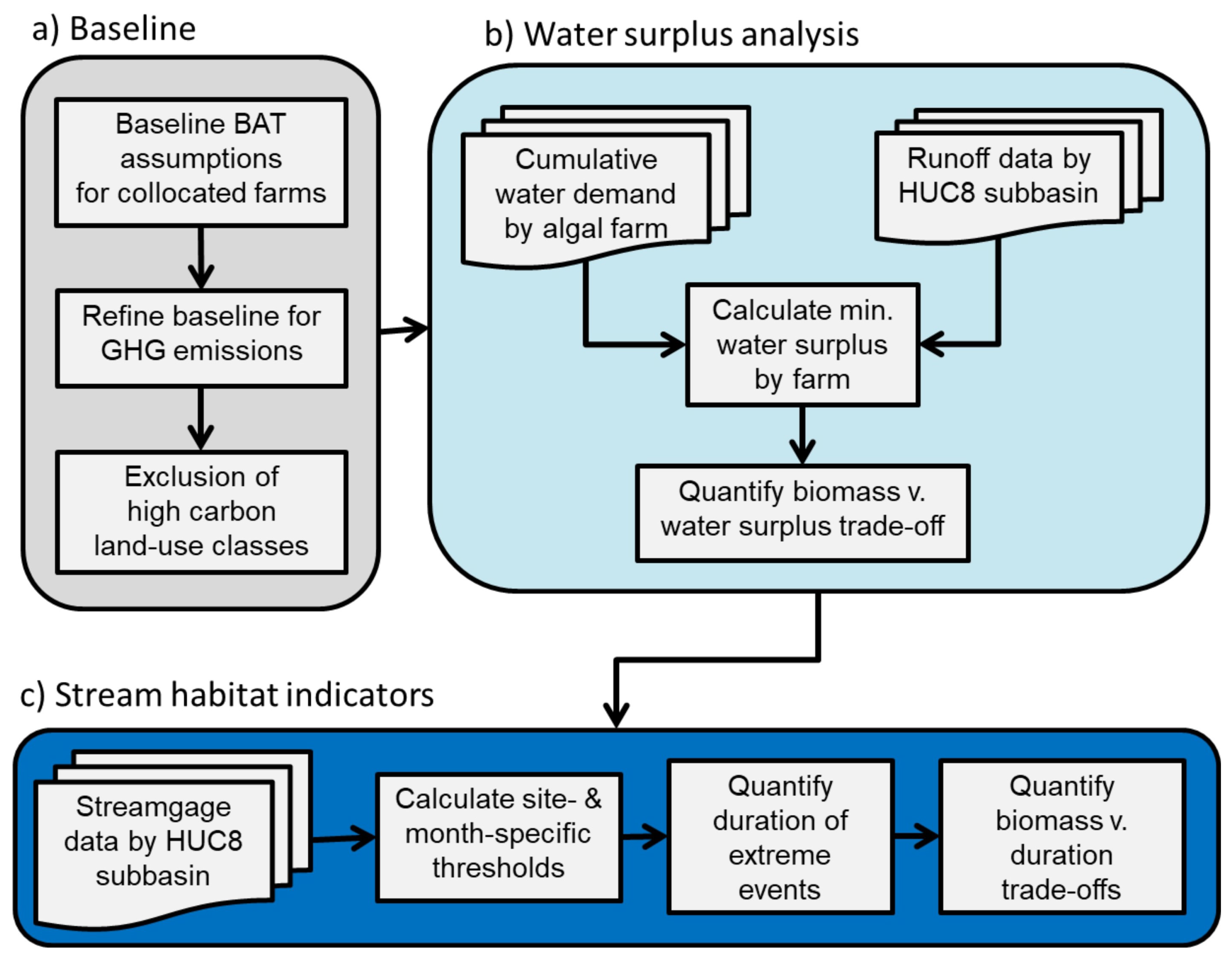
2. Materials and Methods

The approach used here to assess trade-offs between simulated future algal production and associated water stress is illustrated in Figure 1. Building on a previous assessment [47], potential locations for algae production were selected by placing algae ponds near the cheapest sources of waste CO 2 from flue gas and excluding land-use categories with high carbon stocks. After establishing this low-carbon baseline, we totaled monthly water demand from remaining algae farms. Next, we calculated water surplus as a difference between available runoff and demand, and estimated potential biomass under various water surplus thresholds. Finally, we evaluate trade-offs between algae biomass and two indicators of water scarcity (see Supplementary Materials).

2.1. Setting a Low-Carbon Baseline

Establishing a baseline is an important step because it provides context for sustainability indicators [56]. We defined a low-carbon baseline that minimized carbon emissions by avoiding development in lands with high carbon stocks and by capturing waste CO 2 from flue gas. Our analysis assumed that algal biomass would be produced in freshwater open ponds located within a cost-effective distance of waste-CO 2 sources. Researchers from Pacific Northwest National Laboratory (PNNL) used the Biomass Assessment Tool (BAT) model (see Section 2.2) to simulate data for three sources of CO 2 : flue gas from coal-fired power plants, natural-gas power plants, and ethanol-production facilities.
Land competition is often neglected by assessments of production potential for algal biofuels [57]. To address this contribution to the carbon footprint of algae production, we excluded high-carbon-stock lands including forested lands, emergent and herbaceous wetlands, and grasslands from the US National Land Cover Database, NLCD (www.mrlc.gov/national-land-cover-database-nlcd-2016) from modeled algal development. We also excluded wetlands from the 2010 National Wetlands Inventory.
In the sections below, we describe the resource assessment (biomass modeling using the BAT), our assessment of water supply and demand from simulated new algae production, and the implications of water demand by algae for seasonal shortages in water supply and low-flow events in gaged streams.

2.2. Biomass Modeling Using the Biomass Assessment Tool (BAT)

The BAT developed by researchers at PNNL [7,8,58] couples advanced spatial and numerical models to assess resource requirements, land suitability, and biomass and bioenergy potential [8]. BAT was used to model potential algae biomass across the continental US as part of a national bioenergy resource assessment conducted in 2016 [47]. Maps and other visualizations of this assessment can be viewed here: https://bioenergykdf.net/billionton2016/7/1/tableau. The scenario evaluated here assumed current algae productivity [47] at 485.6-ha ‘farms’ with 404.7 ha of open pond algae production (1004.05-ha ponds) [28,47]. We present biomass in units of million US tons, dry weight (Mt). Farm locations were restricted to lands with slopes ≤1% to minimize site preparation, excavation, and operational water pumping costs.
In addition to algae production and cost to obtain waste CO 2 from flue gas, BAT provided estimates of seasonal water demand. The pond temperature and subsequent net consumptive water use (evaporation minus precipitation) for production was modeled using a mass and energy balance model for potential algae production sites across the country [47] using 30 years of hourly stochastic meteorology data and averaged across each state [5]. Biomass growth was modeled for the freshwater algal strain Chlorella sorokiniana at an hourly time-step over a 30-year period using regional estimates of current productivities [47]. More information about the BAT is available [8] and additional model assumptions for the BAT inputs to this analysis are found in [47]. Because BAT was run independently for each CO 2 source, many farms were supplied by the same source and we assumed that supply was not limiting. For each farm, we assigned the source with the least-expensive capital and operational expense annualized costs for source-to-pond CO 2 transport, as calculated by BAT. In cases where two or three sources were equal in cost, the source yielding the highest biomass was selected, with ties broken at random.

2.3. Net Water Availability (Water Surplus)

Water demand was quantified for each algae farm by using BAT. Monthly water demand is primarily due to evaporation, which depends on pond geometry and climate. Next, water supply was estimated for each 8-digit Hydrologic Unit Code subbasin (HUC8) as monthly runoff, R m . For each month m and CO 2 source k, we calculated water demand, d as the sum of evaporation and other consumptive water losses from algal farms located within a given HUC8 subbasin x. We assumed that farms with the highest algal productivity would be constructed first. Let i = 1, ..., n represent the rank order of algae farms from most- to least-productive. With the data thus sorted for each HUC8-watershed and CO 2 source, we calculated cumulative monthly biomass (B i m in Mt, Equation (1)) and cumulative monthly water demand (B i m in ML month 1 , Equation (1)) from ranked farm-specific values. At this point, we selected the least-cost CO 2 source for each subbasin.
B i m = j = 1 i b j m D i m = j = 1 i d j m
Surplus water supply, W was calculated as the difference between monthly runoff for the subbasin, R m and cumulative monthly demand (over farms) (Equation (2)). As an upstream indicator of the risk of seasonal water shortage, we calculated S i , the minimum cumulative water surplus (ML month 1 ) for each set of ranked farms across 12 monthly values (Equation (3)).
W i m = R m D i m
S i = min m = 1 , 12 W i m
We then examined trade-offs between thresholds and algae production by sequentially excluding less-productive farms to meet a threshold for minimum seasonal water surplus in the subbasin. We also produced maps showing the geographic shifts in production as the threshold for surplus water is increased. We developed an interactive visualization of algal supply as a function of the minimum water surplus threshold.

2.4. Implications for Stream Habitat

In the next analysis, we evaluated the effect of setting higher thresholds for water surplus on stream habitat (extreme low flows and high temperatures) in representative streams for each HUC8 basin over the historical period from 1 January 1985 to 31 December 2016. Following the approach described by [10], we characterized extreme events over the historical period of record and selected suitable indicators for low flow and high temperature.
Various measures to characterize low flow are available [59]. The US Geological Survey (USGS) and many states use flow statistics from the past 10 years or more to define low flow, and states often set permit discharge limits based on these statistics [60]. We focus here on the 10th percentile of annual average monthly flow, Qtenn10, an indicator of adequate river flow for biota. For stream temperature, we used the monthly maximum of weekly (7-day) daily average temperature (MWAT) [41,61].
One advantage of duration-based indicators for regional assessments is that they can be more-easily compared across geographic and seasonal contexts, as well as across variables or potential threats, than can flow or thermal indicators that have thresholds derived from particular species of local importance. We hypothesize that species tolerances to the duration of flow and temperature extremes are less region specific (i.e., more canonical) than tolerances to the flows or temperatures themselves. Therefore, we calculated the monthly average duration of either low-flow events (days below-threshold) or monthly average duration of high-temperature events (days above-threshold) from historical data for each river basin with proposed algae biomass farms. This assumes that the most relevant durations are less than 28–31 days. Together, these indicators for stream habitat provided us with the information needed to assess the incidence and severity of water stress in space (HUC8 subbasins) and time (seasons).

2.4.1. Selection of Representative Stream Gages

The BAT model identified 393 subbasins where algae farms could potentially be co-located with CO 2 sources [47]. We identified a representative gage for each subbasin from 3317 USGS gages with historical flow in subbasins with historical flow data. In general, the availability of flow data for the US was far greater than the availability of water temperature data, and availability of gages also varied geographically. The lack of complete national coverage means that we are unable to assess stream habitat conditions for some subbasins with potential algae supply. However, by assuming that gages are ‘missing at random’, we were able to estimate relative changes in biomass availability due to restrictions on the flow indicator for stream habitat.
We included data from the Gages-II dataset, which includes currently active gages with at least 20 years of historical data since 1950 with well-delineated watersheds of <50,000 km 2 in area and intersecting at least one stream segment on a 100-k resolution map [62]. A subset of these were in the USGS Hydroclimatic Data Center dataset of gages with reference watersheds, with minimal alteration of flows [62]. For each HUC8, we favored large mainstem rivers and/or those in the Gages-II dataset. The selected gage within each HUC8 basin is either a Gages-II gage ranked in the top 5 in flow or the non-Gages-II gage with the highest flow. One advantage of linking to Gages-II is the wealth of additional information for these river basins and streams that can be incorporated in future analyses.

2.4.2. Duration of Extreme Stream Habitat Conditions

We identified representative stream gages, where possible, for each HUC8 and evaluated the duration of daily flows below a threshold, i.e., the duration of weekly maximum of daily average temperatures exceeding a threshold monthly MWAT, calculated across years.
To evaluate the potential impact of using these indicators to restrict where algae production facilities are sited, we calculated two relationships. First, we calculated relative reductions in total biomass compared with the total amount when only subbasins with a specified threshold for duration were included. Second, we hypothesized that constraining the location of algae farms based on having an adequate surplus water supply would also reduce the duration of extreme events in streams. Such a negative response in duration would indicate that water surplus would be useful as a ‘master’ or control indicator for impacts to freshwater biota.

3. Results

Below, we present the geographic distribution of indicators including water surplus and indicators of stream habitat. In addition, we present trade-offs between water indicators and algae production, allowing stakeholders to evaluate thresholds that can serve as targets for sustainability.

3.1. Potential Algae Production

The analysis described above estimated that the set of low-carbon algae farms collectively produced 24.8 million tons of biomass. These represent a subset of those identified in the national resource assessment [28], where simulated production was concentrated in the southern states.

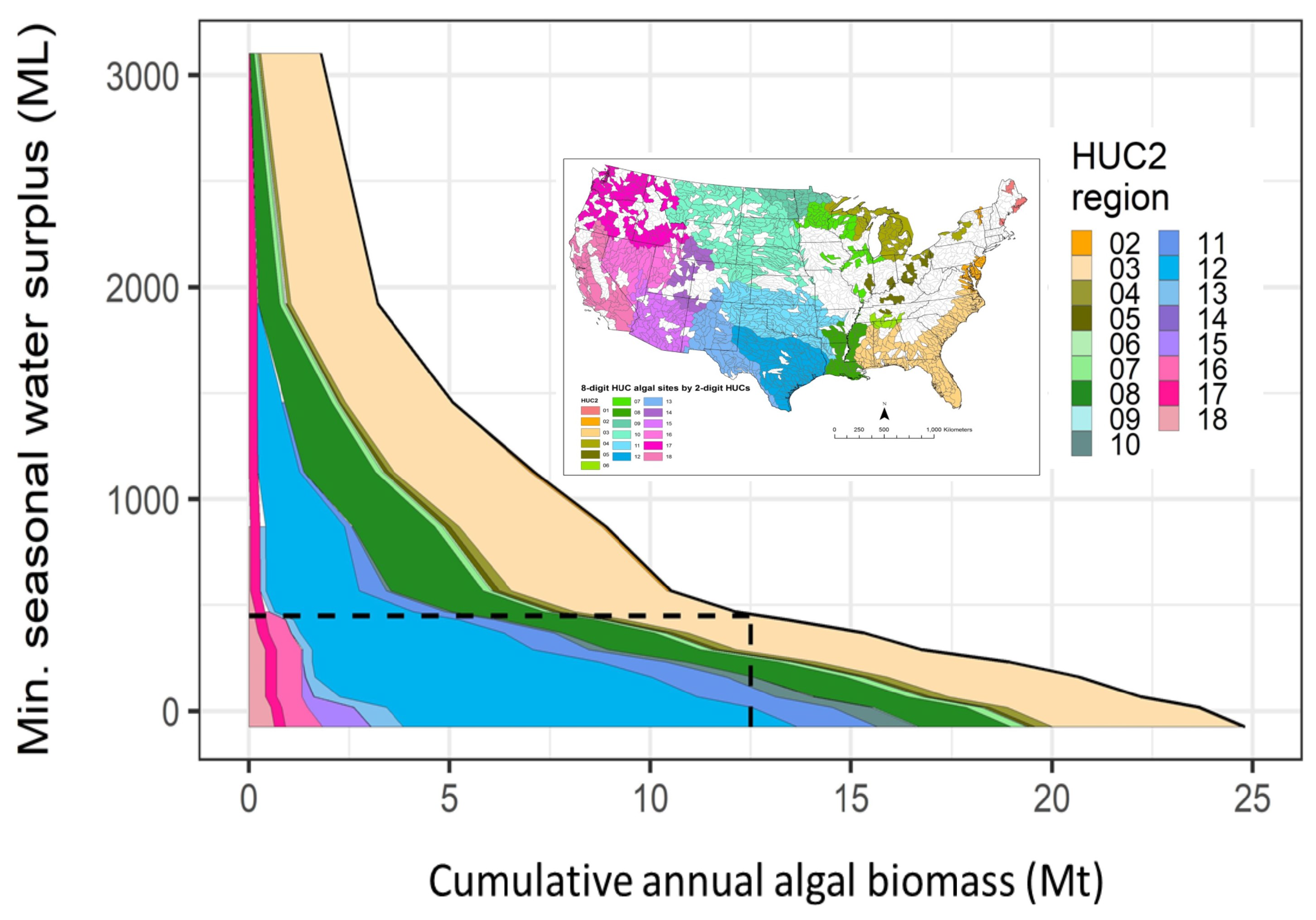
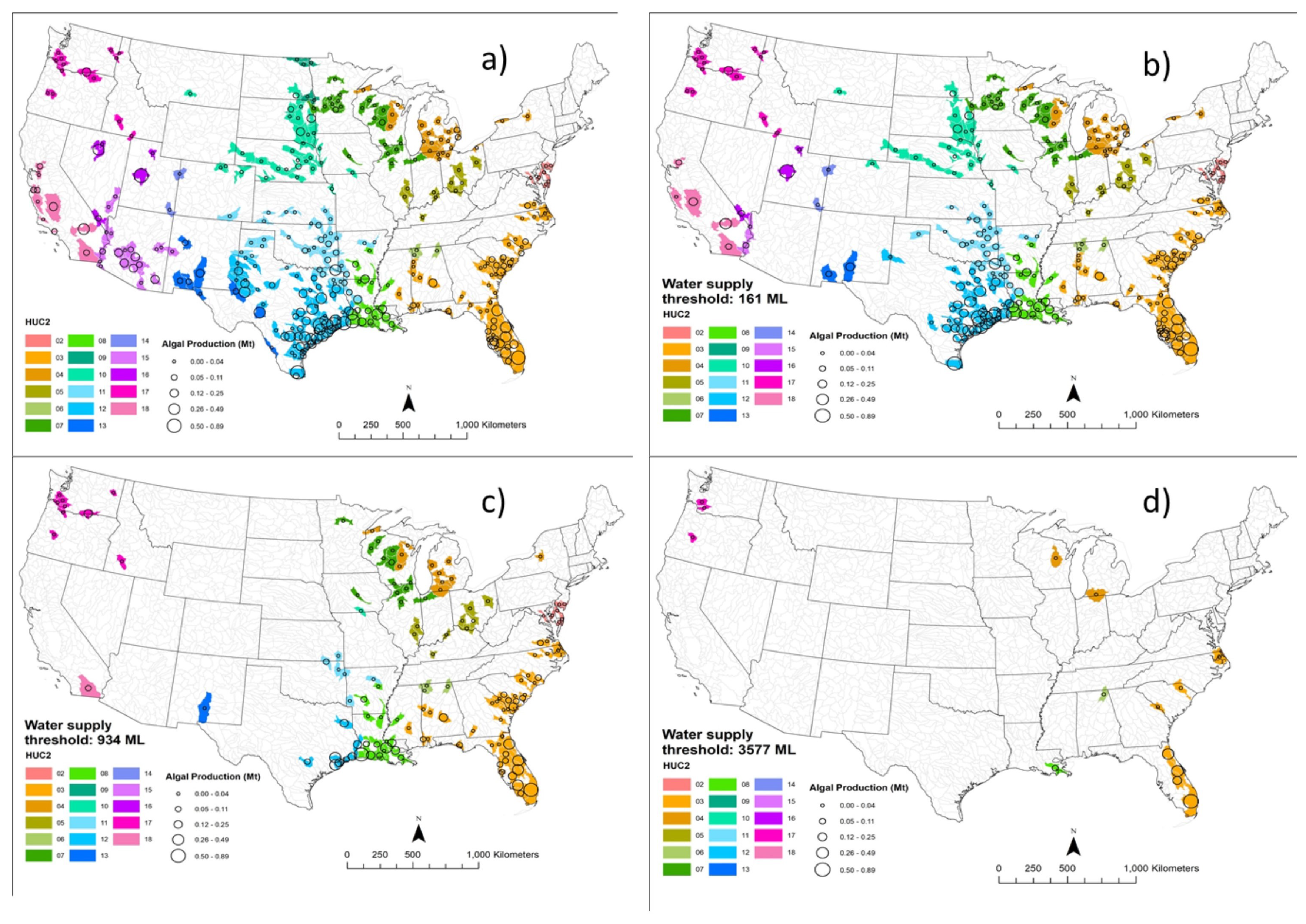
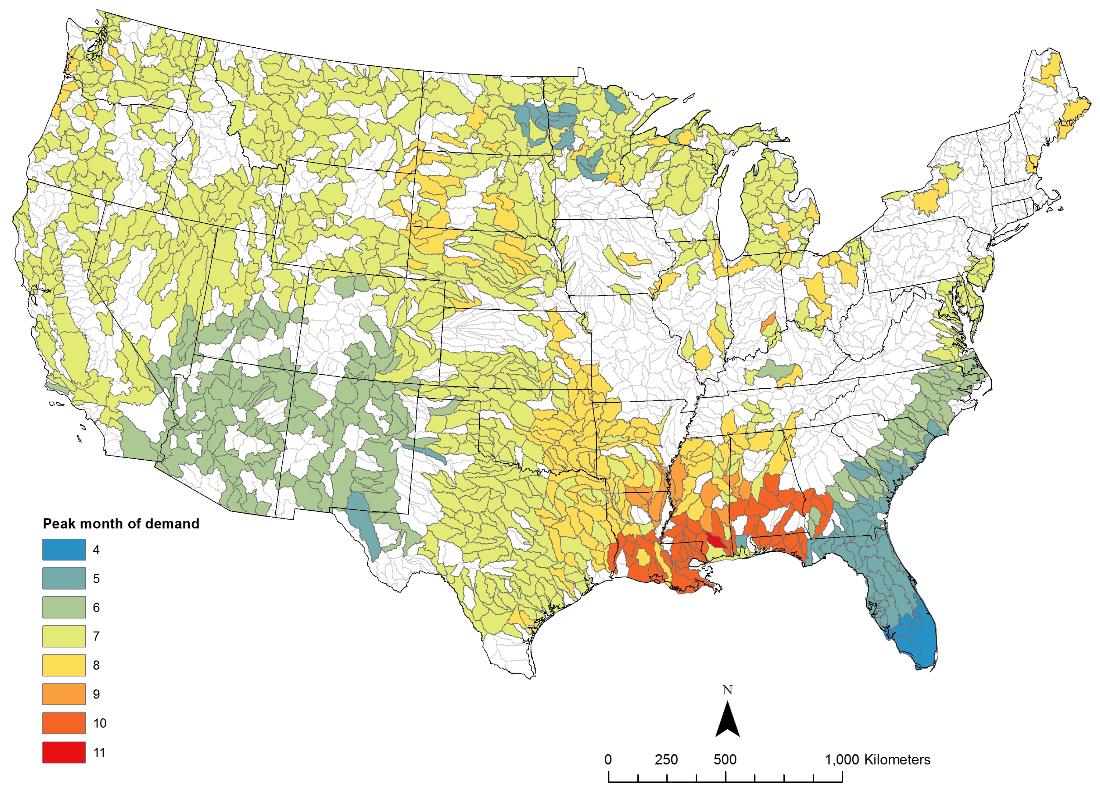
3.2. Net Water Availability (Water Surplus)

Below, we illustrate the trade-off between algae production and the available water surplus (Figure 2). As we lower the threshold water surplus, less-productive farms are excluded, and this has the effect of reducing water demand. A link to an interactive visualization of this trade-off can be found in the Supplemental Information. The four maps in Figure 3 show geographic shifts in the feasibility of producing algal feedstocks under increasingly restricted water surplus (Figure 2). As the required minimum surplus increases (y-axis of Figure 2), sustainable production shifts away from the US southwest and Texas. The Gulf and Florida in the southeastern US persist in providing sustainable algae production when a higher minimum surplus threshold is required (dark green and yellow in Figure 2). The most apparent decrease is in the Midwest, for example, the Rio Grande basin (13), which spans the transition from low precipitation west of the 100th parallel to high precipitation to the east (Figure 2 and Figure 3).
Above we focused on the seasonal minimum surplus, regardless of when (seasonally) that surplus was at a minimum. The timing of water demand also varied geographically (Figure 4). Although summer was the season with peak algae production in most of the conterminous US, subbasins surrounding the Gulf of Mexico (other than Florida) showed peak production in fall, whereas subbasins in Florida peaked in early spring (Figure 4). We projected peak production for the southwest and areas along the southeast Atlantic coast in June (Figure 4).

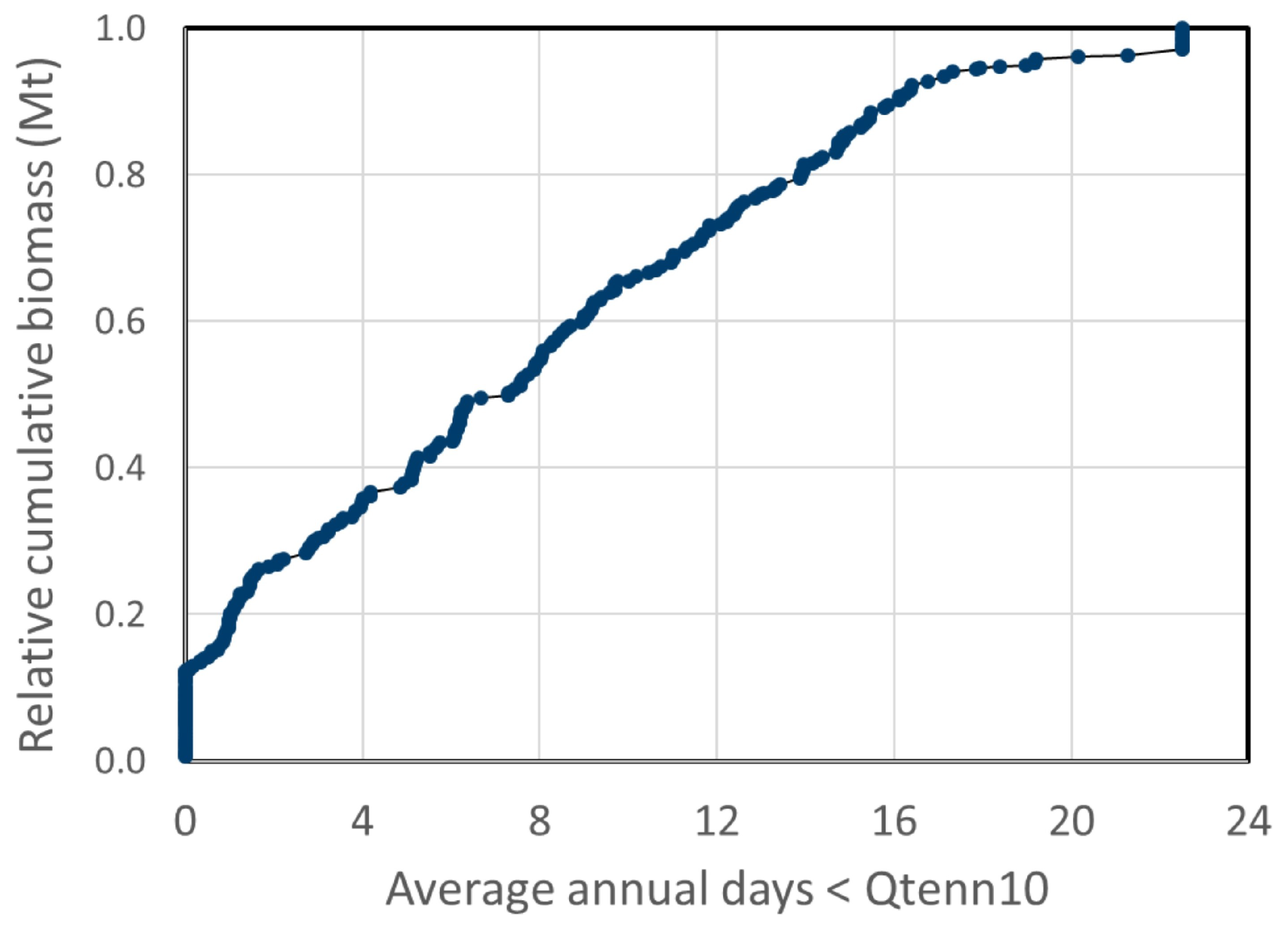
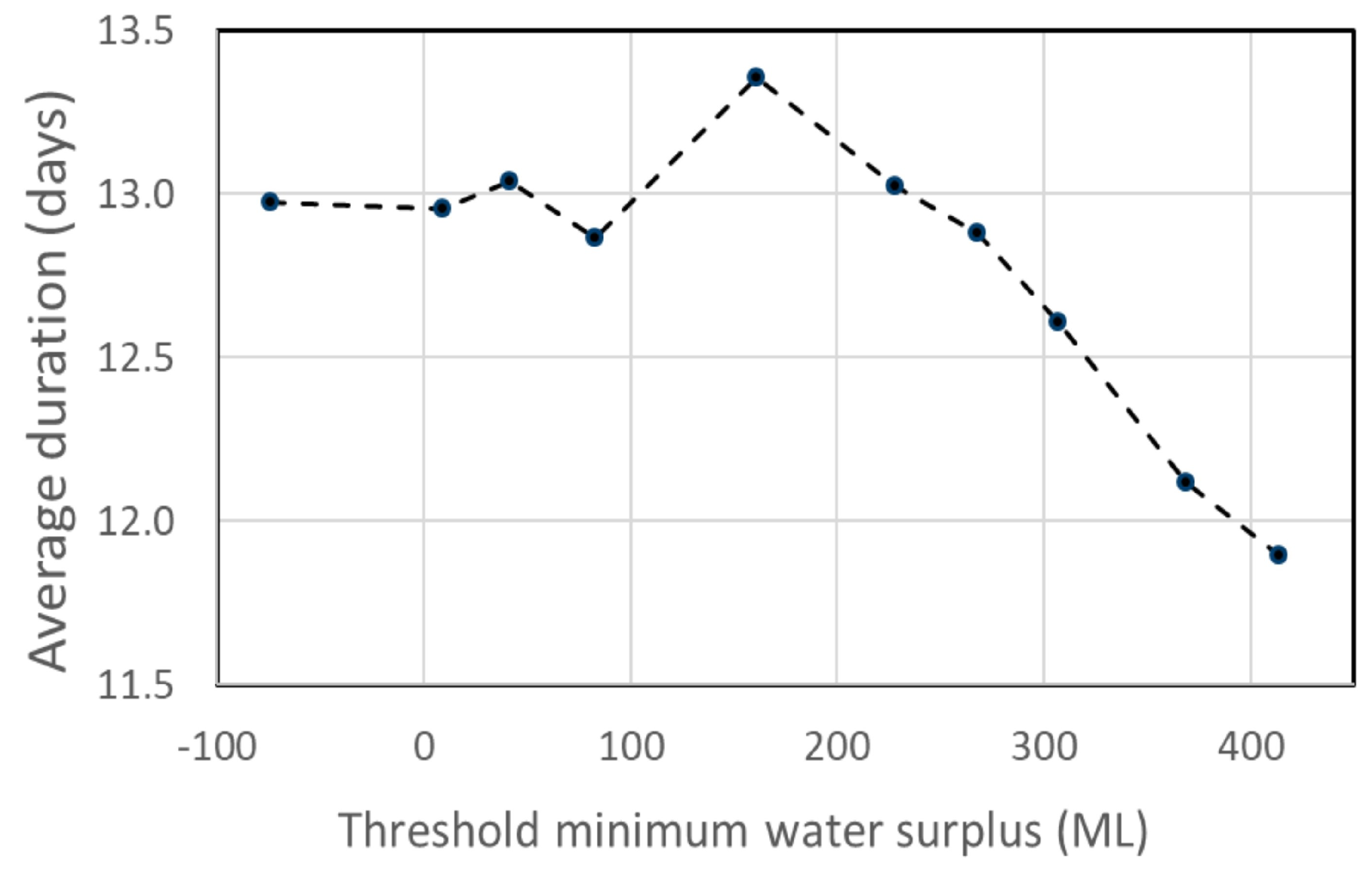
3.3. Implications for Stream Habitat

Low-flow events ranged in duration from zero to a full month (average of 13 days) (Figure 5). In general, when we restricted attention to those HUC8’s with a duration of zero for flows below Qtenn10, the proportional reductions in available biomass were large (Figure 5). Restricting algal development where the minimum water surplus was above 450 ML reduced the available potential biomass by half to roughly 12.5 Mt. Similarly, restricting the duration of low-flow events (<Qtenn10) to 12 day reduced biomass by roughly 75%.
We hypothesized that constraining the number of algae facilities to maintain a threshold water surplus in each HUC8 basin would also improve other sustainability indicators. The average annual duration of low-flow events (Qtenn10) did not vary as much as expected (Figure 6), but we saw the expected decrease in the duration of low-flow events as we constrained water surplus above a minimum seasonal water surplus of 150 ML (Figure 6).

4. Discussion

The environmental sustainability of renewable resources is a priority for energy developers, regulators charged with protecting the environment, and the public. Previous resource analyses have considered potential algal production across the US, and some have considered water availability [4,63]. This study differed in three important ways. First, reducing potential GHG emissions by avoiding high-carbon lands and using waste CO 2 was a prerequisite for candidate sites. Second, we considered the availability of freshwater resources at finer spatial and temporal resolution. We used river basins as natural boundaries and simulated biologically relevant seasonal shortages. Shortages occurred at different times in different regions. Third, we developed ecologically relevant indicators to measure the implications of algal production for stream habitat. We discovered that assessment using water temperature was not possible because there was not enough historical gage data, but we were able to assess low-flow duration.
One sustainability objective for this study was to maintain an adequate water surplus to protect freshwater biota, as inferred from habitat extremes (i.e., streamflow and temperature). We were able to achieve this objective for flow by quantifying changes in the duration of low-flow events attained by limiting the number of algae production facilities. However, to assess thermal effects, additional gages would be needed to monitor stream temperature, especially in regions where algae production is anticipated to be economically most-feasible. One way to view the effects of abstraction that increases heating is as a source of pollution (similar to nitrogen loadings [64]) that additionally converts a portion of the remaining water to grey water (not usable by aquatic biota). However, it is unclear how useful these concepts are when applied to changes in water suitability that are not permanent.
We see several future research needs to build on the analysis pioneered here. Our study focused on algal water demand. Yet, there are other water demands, and the flow and thermal impacts of multiple energy sectors along a river can be expected to have cumulative effects. Furthermore, meeting those demands is, in practice, determined by how systems of reservoirs are operated. Water allocation decisions typically consider a suite of competing demands, some of which have priority over others. For example, water law in the western US follows the doctrine of prior appropriation, which gives precedence to prior users of water [65,66]. Although water rights can be purchased, the doctrine of prior appropriations puts any new industry at a disadvantage in the west [67].
More research is needed to understand the penetration of biodiesel from microalgal production into the set of existing water demands and energy sources, keeping in mind that the energy supplied by algae could offset water demands from displaced fossil or other energy sources. If biodiesel were to replace coal as the fuel source for electricity generation in thermal powerplants (the biggest users of water), water use could potentially increase ([21,68]). Data exist to establish baseline water demands, which are compiled for several sectors of the US economy every five years (see https://water.usgs.gov/watuse/) [69] by county. In practice, integrating water demands would be achieved through changes in more-or-less coordinated operations of multiple reservoirs by individual owners constrained by hydropower licenses, water quality requirements, and regional water law.
We adopted economic assumptions from the PNNL BAT modeling analysis that could be further refined. For example, additional waste-CO 2 sources, such as ammonia plants and cement plants, could potentially support additional algae production. Secondly, algae ponds will become more productive with new technologies and strains. However, higher productivity could also reduce the amount of cost-effective waste-CO 2 resource. One analysis indicated that transporting dilute CO 2 in flue gas from natural-gas power plants would not be cost-effective once algal productivities doubled to about 25 g m 2 day 1 [70]. This is because of the added cost of larger pipes required to carry more gas [70]. In addition, land cost is an important economic constraint [71] that we did not consider.
We identified spatial patterns in the areas where algae production remains possible for different minimum water surplus thresholds. Clearly, some HUC8 river basins could offer a more-sustainable combination of algae productivity and water availability than others. However, in more arid regions, where water is overallocated, alternative production methods may be needed to supply biofuels. For example, photobioreactors are an alternative with lower evaporation rates than production in open ponds, but they are more expensive to operate. Furthermore, photobioreactors can allow production in basins with plentiful water and in cooler climates (if waste heat from industrial processes is used) [72]. Finally, replacing potable with non-potable water sources could, by one estimate, save 90% of freshwater requirements [24]. Municipal wastewater use is another sustainable option for water-constrained regions [30,73]. In addition, tens of millions of tons of algae can be produced from saline waters in the US under similar CO 2 co-location constraints as in this study and using Nannochloropsis salina as the model strain [6,47,74]. However, saline biomass has additional costs [75,76] including those associated with developing infrastructure and disposing of wastewater.

5. Conclusions

In this study, we established a new baseline that considers the carbon footprint of algae production in the conterminous US, and we defined and evaluated sustainability indicators related to water consumption and stress to freshwater habitat. We evaluated trade-offs between potential algal biomass production and preservation of adequate surplus water and instream flows to protect aquatic habitat. The low-carbon baseline resulted in around 25 million US (metric) tons of algae, with lower production as restrictions on surplus water increase (Figure 2). Our results highlight regions where seasonal water surpluses are high as most promising for sustainable algae production. Areas with a sufficient water surplus are widespread, suggesting that freshwater should not be a significant constraint on future algae production for energy in those locations. In areas where freshwater is constrained, alternative water sources or production systems that minimize evaporation (e.g., photobioreactors) can be considered.

Supplementary Materials

The following are available online at https://www.mdpi.com/2073-4441/11/4/836/s1, Visualization of trade-offs between water surplus and algal biomass https://cbes.ornl.gov/data-visualizations/.

Author Contributions

Conceptualization, R.A.E. and H.I.J.; methodology, H.I.J.; formal analysis, H.I.J.; data curation, L.M.B.; writing—original draft preparation, H.I.J.; writing—review and editing, H.I.J. and R.A.E., L.M.B.; visualization, H.I.J.; project administration, R.A.E.; funding acquisition, R.A.E.

Funding

We thank Department of Energy’s (DOE) Bioenergy Technologies Office and Devinn Lambert, program manager for funding this work. Part of this this research, carried out at the Jet Propulsion Laboratory, California Institute of Technology, was under a contract with the National Aeronautics and Space Administration, copyright 2018 California Institute of Technology.

Acknowledgments

We greatly appreciate Andre Coleman and Mark Wigmosta (PNNL) for their collaboration in this research, which included providing BAT simulation results for our analysis. This manuscript has been authored by UT-Battelle, LLC under Contract No. DE-AC05-00OR22725 with the US DOE. The United States Government retains and the publisher, by accepting the article for publication, acknowledges that the United States Government retains a non-exclusive, paid-up, irrevocable, world-wide license to publish or reproduce the published form of this manuscript, or allow others to do so, for United States Government purposes. The Department of Energy will provide public access to these results of federally sponsored research in accordance with the DOE Public Access Plan (http://energy.gov/downloads/doe-public-access-plan). We appreciate a collegial review by Teresa Mathews and reviews by two anonymous reviewers.

Conflicts of Interest

The authors declare no conflict of interest. The funders had no role in the design of the study; in the collection, analyses, or interpretation of data; in the writing of the manuscript, or in the decision to publish the results.

References

  1. Mohtar, R.H.; Shafiezadeh, H.; Blake, J.; Daher, B. Economic, social, and environmental evaluation of energy development in the Eagle Ford shale play. Sci. Total Environ. 2019, 646, 1601–1614. [Google Scholar] [CrossRef] [PubMed]
  2. Daher, B.; Lee, S.H.; Kaushik, V.; Blake, J.; Askariyeh, M.H.; Shafiezadeh, H.; Zamaripa, S.; Mohtar, R.H. Towards bridging the water gap in Texas: A water-energy-food nexus approach. Sci. Total Environ. 2019, 647, 449–463. [Google Scholar] [CrossRef] [PubMed]
  3. Tan, J.; Tan, R.R.; Aviso, K.B.; Promentilla, M.A.B.; Sulaiman, N.M.N. Study of microalgae cultivation systems based on integrated analytic hierarchy process-life cycle optimization. Clean Technol. Environ. Policy 2017, 19, 2075–2088. [Google Scholar] [CrossRef]
  4. Venteris, E.R.; Skaggs, R.L.; Wigmosta, M.S.; Coleman, A.M. A national-scale comparison of resource and nutrient demands for algae-based biofuel production by lipid extraction and hydrothermal liquefaction. Biomass Bioenergy 2014, 64, 276–290. [Google Scholar] [CrossRef]
  5. Venteris, E.R.; McBride, R.C.; Coleman, A.M.; Skaggs, R.L.; Wigmosta, M.S. Siting Algae Cultivation Facilities for Biofuel Production in the United States: Trade-Offs between Growth Rate, Site Constructability, Water Availability, and Infrastructure. Environ. Sci. Technol. 2014, 48, 3559–3566. [Google Scholar] [CrossRef] [PubMed]
  6. Venteris, E.R.; Skaggs, R.L.; Coleman, A.M.; Wigmosta, M.S. A GIS cost model to assess the availability of freshwater, seawater, and saline groundwater for algal biofuel production in the United States. Environ. Sci. Technol. 2013, 47, 4840–4849. [Google Scholar] [CrossRef]
  7. Wigmosta, M.S.; Coleman, A.M.; Skaggs, R.J.; Huesemann, M.H.; Lane, L.J. National microalgae biofuel production potential and resource demand. Water Resour. Res. 2011, 47. [Google Scholar] [CrossRef] [Green Version]
  8. Coleman, A.M.; Abodeely, J.M.; Skaggs, R.L.; Moeglein, W.A.; Newby, D.T.; Venteris, E.R.; Wigmosta, M.S. An integrated assessment of location-dependent scaling for microalgae biofuel production facilities. Algal Res. 2014, 5, 79–94. [Google Scholar] [CrossRef]
  9. Baumber, A. Enhancing ecosystem services through targeted bioenergy support policies. Ecosyst. Serv. 2017, 26, 98–110. [Google Scholar] [CrossRef]
  10. Jager, H.I.; Efroymson, R.A. Can upstream biofuel production increase the flow of downstream ecosystem goods and services? Biomass Bioenergy 2018, 114, 125–131. [Google Scholar] [CrossRef]
  11. Selosse, S.; Ricci, O. Carbon capture and storage: Lessons from a storage potential and localization analysis. Appl. Energy 2017, 188, 32–44. [Google Scholar] [CrossRef]
  12. Edmundson, S.J.; Wilkie, A.C. Landfill leachate—A water and nutrient resource for algae-based biofuels. Environ. Technol. 2013, 34, 1849–1857. [Google Scholar] [CrossRef] [PubMed]
  13. Norvill, Z.N.; Shilton, A.; Guieysse, B. Emerging contaminant degradation and removal in algal wastewater treatment ponds: Identifying the research gaps. J. Hazard. Mater. 2016, 313, 291–309. [Google Scholar] [CrossRef] [PubMed]
  14. Raven, J.A. The possible roles of algae in restricting the increase in atmospheric CO2 and global temperature. Eur. J. Phycol. 2017, 52, 506–522. [Google Scholar] [CrossRef]
  15. Vasseur, C.; Bougaran, G.; Garnier, M.; Hamelin, J.; Leboulanger, C.; Le Chevanton, M.; Mostajir, B.; Sialve, B.; Steyer, J.P.; Fouilland, E. Carbon conversion efficiency and population dynamics of a marine algae-bacteria consortium growing on simplified synthetic digestate: First step in a bioprocess coupling algal production and anaerobic digestion. Bioresour. Technol. 2012, 119, 79–87. [Google Scholar] [CrossRef]
  16. US Department of Energy Efroymson (Lead). Billion Ton 2016 Report: Volume II. Environmental Effects; Oak Ridge National Laboratory: Oak Ridge, TN, USA, 2016.
  17. Gerbens-Leenes, P.W.; Xu, L.; de Vries, G.J.; Hoekstra, A.Y. The blue water footprint and land use of biofuels from algae. Water Resour. Res. 2014, 50, 8549–8563. [Google Scholar] [CrossRef] [Green Version]
  18. Kasischke, E.S.; Amiro, B.D.; Barger, N.N.; French, N.H.F.; Goetz, S.J.; Grosse, G.; Harmon, M.E.; Hicke, J.A.; Liu, S.G.; Masek, J.G. Impacts of disturbance on the terrestrial carbon budget of North America. J. Geophys. Res. Biogeosci. 2013, 118, 303–316. [Google Scholar] [CrossRef] [Green Version]
  19. Medeiros, D.L.; Sales, E.A.; Kiperstok, A. Energy production from microalgae biomass: Carbon footprint and energy balance. J. Clean. Prod. 2015, 96, 493–500. [Google Scholar] [CrossRef]
  20. Yeh, S.; Berndes, G.; Mishra, G.S.; Wani, S.P.; Neto, A.E.; Suh, S.; Karlberg, L.; Heinke, J.; Garg, K.K. Evaluation of water use for bioenergy at different scales. Biofuels Bioprod. Biorefin. 2011, 5, 361–374. [Google Scholar] [CrossRef]
  21. Gerbens-Leenes, W.; Hoekstra, A.Y.; van der Meer, T.H. The water footprint of bioenergy. Proc. Natl. Acad. Sci. USA 2009, 106, 10219–10223. [Google Scholar] [CrossRef] [Green Version]
  22. Berndes, G. Future biomass energy supply: The consumptive water use perspective. Int. J. Water Resour. Dev. 2008, 24, 235–245. [Google Scholar] [CrossRef]
  23. Frank, E.D.; Elgowainy, A.; Han, J.; Wang, Z.C. Life cycle comparison of hydrothermal liquefaction and lipid extraction pathways to renewable diesel from algae. Mitig. Adapt. Strateg. Glob. Chang. 2013, 18, 137–158. [Google Scholar] [CrossRef]
  24. Yang, J.; Xu, M.; Zhang, X.Z.; Hu, Q.A.; Sommerfeld, M.; Chen, Y.S. Life-cycle analysis on biodiesel production from microalgae: Water footprint and nutrients balance. Bioresour. Technol. 2011, 102, 159–165. [Google Scholar] [CrossRef] [PubMed]
  25. Canter, C.E.; Davis, R.; Urgun-Demirtas, M.; Frank, E.D. Infrastructure associated emissions for renewable diesel production from microalgae. Algal Res. 2014, 5, 195–203. [Google Scholar] [CrossRef]
  26. Slade, R.; Bauen, A. Micro-algae cultivation for biofuels: Cost, energy balance, environmental impacts and future prospects. Biomass Bioenergy 2013, 53, 29–38. [Google Scholar] [CrossRef] [Green Version]
  27. Rogers, J.N.; Rosenberg, J.N.; Guzman, B.J.; Oh, V.H.; Mimbela, L.E.; Ghassemi, A.; Betenbaugh, M.J.; Oyler, G.A.; Donohue, M.D. A critical analysis of paddlewheel-driven raceway ponds for algal biofuel production at commercial scales. Algal Res. 2014, 4, 76–88. [Google Scholar] [CrossRef] [Green Version]
  28. Efroymson, R.; Coleman, A.; Wigmosta, M.; Pattullo, M.; Mayes, M.; Langholtz, M. Qualitative Analysis of Environmental Effects of Algae Production; Report ORNL/TM-2016/727; Oak Ridge National Laboratory: Oak Ridge, TN, USA, 2017. [Google Scholar] [CrossRef]
  29. Shurin, J.B.; Mandal, S.; Abbott, R.L. Trait diversity enhances yield in algal biofuel assemblages. J. Appl. Ecol. 2014, 51, 603–611. [Google Scholar] [CrossRef] [Green Version]
  30. Arita, C.Q.; Yilmaz, O.; Barlak, S.; Catton, K.B.; Quinn, J.C.; Bradley, T.H. A geographical assessment of vegetation carbon stocks and greenhouse gas emissions on potential microalgae-based biofuel facilities in the United States. Bioresour. Technol. 2016, 221, 270–275. [Google Scholar] [CrossRef] [PubMed] [Green Version]
  31. Davis, R.; Wu, W.H.; Tran-Gyamfi, M.; Lane, T.; Pate, R.; Wu, B. Comprehensive bioconversion of algae to liquid fuels and intermediate value products. In Abstracts of Papers of the American Chemical Society; American Chemical Society: Washington, DC, USA, 2016; Volume 251. [Google Scholar]
  32. De Maria, P.D. On the Use of Seawater as Reaction Media for Large-Scale Applications in Biorefineries. Chemcatchem 2013, 5, 1643–1648. [Google Scholar] [CrossRef]
  33. Oki, T.; Kanae, S. Global hydrological cycles and world water resources. Science 2006, 313, 1068–1072. [Google Scholar] [CrossRef]
  34. Brauman, K.A.; Richter, B.D.; Postel, S.; Malsy, M.; Flörke, M. Water depletion: An improved metric for incorporating seasonal and dry-year water scarcity into water risk assessments. Elem. Sci. Anthr. 2016, 4, 000083. [Google Scholar] [CrossRef] [Green Version]
  35. Helmbrecht, J.; Pastor, J.; Moya, C. Smart solution to improve water-energy nexus for water supply systems. Procedia Eng. 2017, 186, 101–109. [Google Scholar] [CrossRef]
  36. Garbe, J.; Beevers, L.; Pender, G. Valuing the Effect of Freshwater Over-abstraction on Fish Species. In Proceedings of the 35th IAHR World Congress, Vols I and II; International Association for Hydro-Environment Engineering and Research (IAHR): Madrid, Spain; 2013; pp. 2769–2778. [Google Scholar]
  37. Poff, N.L.; Allan, J.D.; Bain, M.B.; Karr, J.R.; Prestegaard, K.L.; Richter, B.D.; Sparks, R.E.; Stromberg, J.C. The natural flow regime. BioScience 1997, 47, 769–784. [Google Scholar] [CrossRef]
  38. Olden, J.D.; Poff, N.L. Redundancy and the choice of hydrologic indices for characterizing streamflow regimes. River Res. Appl. 2003, 19, 101–121. [Google Scholar] [CrossRef]
  39. McManamay, R.A.; Brewer, S.; Jager, H.I.; Troia, M.J. Organizing environmental flow frameworks to meet hydropower mitigation needs. Environ. Manag. 2016, 58, 365–385. [Google Scholar] [CrossRef]
  40. Poff, N.L.; Richter, B.D.; Arthington, A.H.; Bunn, S.E.; Naiman, R.J.; Kendy, E.; Acreman, M.; Apse, C.; Bledsoe, B.P.; Freeman, M.C.; et al. The ecological limits of hydrologic alteration (ELOHA): A new framework for developing regional environmental flow standards. Freshw. Biol. 2010, 55, 147–170. [Google Scholar] [CrossRef]
  41. McCullough, D.A. Are coldwater fish populations of the United States actually being protected by temperature standards? Freshw. Rev. 2010, 3, 147–197. [Google Scholar] [CrossRef]
  42. Richter, A.; Kolmes, S.A. Maximum temperature limits for chinook, coho, and chum salmon, and steelhead trout in the Pacific Northwest. Rev. Fish. Sci. 2005, 13, 23–49. [Google Scholar] [CrossRef]
  43. Nadeau, T.L.; Leibowitz, S.G.; Wigington, P.J., Jr.; Ebersole, J.L.; Fritz, K.M.; Coulombe, R.A.; Comeleo, R.L.; Blocksom, K.A. Validation of rapid assessment methods to determine streamflow duration classes in the Pacific Northwest, USA. Environ. Manag. 2015, 56, 34–53. [Google Scholar] [CrossRef]
  44. Jager, H. Thinking outside the channel: Timing pulse flows to benefit salmon via indirect pathways. Ecol. Model. 2014, 217, 117–127. [Google Scholar] [CrossRef]
  45. McCullough, D.A.; Bartholow, J.M.; Jager, H.I.; Beschta, R.L.; Cheslak, E.F.; Deas, M.L.; Ebersole, J.L.; Foott, J.S.; Johnson, S.L.; Marine, K.R.; et al. Research in thermal biology: Burning questions for coldwater stream fishes. Rev. Fish. Sci. 2009, 17, 90–115. [Google Scholar] [CrossRef]
  46. Eaton, J.G.; Scheller, R.M. Effects of climate warming on fish thermal habitat in streams of the United States. Limnol. Oceanogr. 1996, 41, 1109–1115. [Google Scholar] [CrossRef] [Green Version]
  47. Efroymson, R.; Coleman, A.; Wigmosta, M.; Schoenung, S.; Sokhansanj, S.; Langholtz, M.; Davis, M. 2016 Billion-Ton Report: Advancing Domestic Resources for a Thriving Bioeconomy, Volume 1: Economic Availability of Feedstocks; Langholtz, M., Stokes, B., Eaton, L., Eds.; ORNL/TM-2016/160; Oak Ridge National Laboratory: Oak Ridge, TN, USA, 2016; Book Section 7; p. 448. [Google Scholar]
  48. Perkin, J.S.; Gido, K.B.; Costigan, K.H.; Daniels, M.D.; Johnson, E.R. Fragmentation and drying ratchet down Great Plains stream fish diversity. Aquat. Conserv. Mar. Freshw. Ecosyst. 2015, 25, 639–655. [Google Scholar] [CrossRef]
  49. Mistak, J.L.; Hayes, D.B.; Bremigan, M.T. Food habits of coexisting salmonines above and below Stronach Dam in the Pine River, Michigan. Environ. Biol. Fishes 2003, 67, 179–190. [Google Scholar] [CrossRef]
  50. Jager, H.I.; King, A.W.; Gangrade, S.; Haines, A.; DeRolph, C.; Naz, B.S.; Ashfaq, M. Will future climate change increase the risk of violating minimum flow and maximum temperature thresholds below dams in the Pacific Northwest? Clim. Risk Manag. 2018, 21, 69–84. [Google Scholar] [CrossRef]
  51. Olden, J.D.; Naiman, R.J. Incorporating thermal regimes into environmental flows assessments: modifying dam operations to restore freshwater ecosystem integrity. Freshw. Biol. 2010, 55, 86–107. [Google Scholar] [CrossRef]
  52. Sesma-Martin, D. The river’s light: Water needs for thermoelectric power generation in the Ebro River basin, 1969–2015. Water 2019, 11, 441. [Google Scholar] [CrossRef]
  53. Cook, M.A.; King, C.W.; Webber, M.E. Implications of Thermal Discharge Limits On Future Power Generation in Texas. In Proceedings of the Asme International Mechanical Engineering Congress and Exposition, San Diego, CA, USA, 15–21 November 2013; ASME International Mechanical Engineering Congress and Exposition: San Diego, CA, USA, 2014; Volume 6b. [Google Scholar]
  54. Stewart, R.J.; Wollheim, W.M.; Miara, A.; Vorosmarty, C.J.; Fekete, B.; Lammers, R.B.; Rosenzweig, B. Horizontal cooling towers: Riverine ecosystem services and the fate of thermoelectric heat in the contemporary Northeast US. Environ. Res. Lett. 2013, 8, 025010. [Google Scholar] [CrossRef]
  55. Cook, M.A.; King, C.W.; Davidson, F.T.; Webber, M.E. Assessing the impacts of droughts and heat waves at thermoelectric power plants in the United States using integrated regression, thermodynamic, and climate models. Energy Rep. 2015, 1, 193–203. [Google Scholar] [CrossRef] [Green Version]
  56. Efroymson, R.; Dale, V. Environmental indicators for sustainable production of algal biofuels. Ecol. Indic. 2015, 49, 1–13. [Google Scholar] [CrossRef] [Green Version]
  57. Lopez-Diaz, D.C.; Lira-Barragan, L.F.; Rubio-Castro, E.; Ponce-Ortega, J.M.; El-Halwagi, M.M. Optimal location of biorefineries considering sustainable integration with the environment. Renew. Energy 2017, 100, 65–77. [Google Scholar] [CrossRef]
  58. Huesemann, M.; Crowe, B.; Waller, P.; Chavis, A.; Hobbs, S.; Edmundson, S.; Wigmosta, M. A validated model to predict microalgae growth in outdoor pond cultures subjected to fluctuating light intensities and water temperatures. Algal Res. 2016, 13, 195–206. [Google Scholar] [CrossRef] [Green Version]
  59. Smakhtin, V.U. Low flow hydrology: A review. J. Hydrol. 2001, 240, 147–186. [Google Scholar] [CrossRef]
  60. Reilly, C.F.; Kroll, C.N. Estimation of 7-day, 10-year low-streamflow statistics using baseflow correlation. Water Resour. Res. 2003, 39. [Google Scholar] [CrossRef] [Green Version]
  61. Essig, D.; Mebane, C.; Hillman, T. Update of Bull Trout Temperature Requirements; Idaho Department of Environmental Quality: Boise, Idaho, 2003. [Google Scholar]
  62. Falcone, J. GAGES II (Geospatial Attributes of Gages for Evaluating Streamflow) Summary Report; USGS: Reston, VA, USA, 2011.
  63. Xu, H.; Lee, U.; Coleman, A.M.; Wigmosta, M.S.; Wang, M. Assessment of algal biofuel resource potential in the United States with consideration of regional water stress. Algal Res. 2019, 37, 30–39. [Google Scholar] [CrossRef]
  64. Mekonnen, M.M.; Hoekstra, A.Y. Global Gray Water Footprint and Water Pollution Levels Related to Anthropogenic Nitrogen Loads to Fresh Water. Environ. Sci. Technol. 2015, 49, 12860–12868. [Google Scholar] [CrossRef] [PubMed]
  65. Loehman, E.T.; Charney, S. Further down the road to sustainable environmental flows: Funding, management activities and governance for six western US states. Water Int. 2011, 36, 873–893. [Google Scholar] [CrossRef]
  66. Null, S.E.; Prudencio, L. Climate change effects on water allocations with season dependent water rights. Sci. Total Environ. 2016, 571, 943–954. [Google Scholar] [CrossRef]
  67. Podolak, C.J.P.; Doyle, M. Conditional water rights in the western United States: Introducting uncertainty to prior appropriation? J. Am. Water Resour. Assoc. 2015, 51, 14–32. [Google Scholar] [CrossRef]
  68. Hadian, S.; Madani, K. A system of systems approach to energy sustainability assessment: Are all renewables really green? Ecol. Indic. 2015, 52, 194–206. [Google Scholar] [CrossRef]
  69. Dieter, C.; Maupin, M.; Caldwell, R.; Harris, M.; Ivahnenko, T.; Lovelace, J.; Barber, N.; Linsey, K. Estimated Use of Water in the United States in 2015; Report U.S. Geological Survey Circular 1441; US Geological Survey: Cantonsville, MD, USA, 2018. [CrossRef]
  70. Schoenung, S.; Efroymson, R.; Langholtz, M. Considerations for the Design of a Gas Transport System for Co-Location of Microalgae Cultivation with CO2 Sources; Technical Report; Oak Ridge National Laboratory: Oak Ridge, TN, USA, 2019. [Google Scholar]
  71. Sharma, B.; Brandes, E.; Khanchi, A.; Birrell, S.; Heaton, E.; Miguez, F.E. Evaluation of Microalgae Biofuel Production Potential and Cultivation Sites Using Geographic Information Systems: A Review. Bioenergy Res. 2015, 8, 1714–1734. [Google Scholar] [CrossRef]
  72. Laamanen, C.A.; Shang, H.L.; Ross, G.M.; Scott, J.A. A model for utilizing industrial off-gas to support microalgae cultivation for biodiesel in cold climates. Energy Convers. Manag. 2014, 88, 476–483. [Google Scholar] [CrossRef]
  73. Zhao, X.B.; Yan, W.; Wang, Y.Q.; Lu, W.; Ma, S. Simulation study on the design of key technical parameters in marine environment sounding with fully polarimetric synthetic aperture radar based on ocean surface scattering model. Acta Phys. Sin. 2014, 63, 21. [Google Scholar] [CrossRef]
  74. Bennett, M.C.; Turn, S.Q.; Chan, W.Y. A methodology to assess open pond, phototrophic, algae production potential: A Hawaii case study. Biomass Bioenergy 2014, 66, 168–175. [Google Scholar] [CrossRef]
  75. Resurreccion, E.P.; Colosi, L.M.; White, M.A.; Clarens, A.F. Comparison of algae cultivation methods for bioenergy production using a combined life cycle assessment and life cycle costing approach. Bioresour. Technol. 2012, 126, 298–306. [Google Scholar] [CrossRef] [PubMed]
  76. Davis, R.E.; Fishman, D.B.; Frank, E.D.; Johnson, M.C.; Jones, S.B.; Kinchin, C.M.; Skaggs, R.L.; Venteris, E.R.; Wigmosta, M.S. Integrated Evaluation of Cost, Emissions, and Resource Potential for Algal Biofuels at the National Scale. Environ. Sci. Technol. 2014, 48, 6035–6042. [Google Scholar] [CrossRef] [PubMed]
Figure 1. Process used to assess the marginal sustainability outcomes for increased water demand associated with algae production. Primary steps included (a) establishing a low-carbon baseline, (b) defining and assessing how thresholds for minimum water surplus influence potential US algae production, and (c) assessing the duration of extreme low-flow and high-temperature events in representative streams.
Water 11 00836 g001
Figure 2. Simulated algal production declined from 24.8 Mt to 1.8 Mt as the threshold for minimum seasonal surplus freshwater increases from a deficit of 74 ML to a surplus of 3106 ML. The dotted lines show the total annual biomass of around 12.5 Mt when restricting within-subbasin algae development such that a surplus of 450 ML remains. Colors of HUC2 basins in the inset map correspond with stacked curves.
Water 11 00836 g002
Figure 3. Geographic shifts in areas where algae can be produced sustainably with respect to constraints on freshwater supply. Threshold values for minimum seasonal (monthly) water surplus. shown are (a) −74 ML (deficit), (b) 161 ML, (c) 934 ML, and (d) 3577 ML.
Water 11 00836 g003
Figure 4. Month of peak water demand due to evaporation from open ponds for each HUC8.
Water 11 00836 g004
Figure 5. Cumulative increase in relative biomass supply as the duration of events increased for subbasins with gage data for streamflow.
Water 11 00836 g005
Figure 6. Change in the duration of events below low-flow threshold Qtenn10 as the threshold for minimum seasonal water surplus increased.
Water 11 00836 g006

