MILP for Optimizing Water Allocation and Reservoir Location: A Case Study for the Machángara River Basin, Ecuador

Abstract

The allocation of water flowing through a river-with-reservoirs system to optimally meet spatially distributed and temporally variable demands can be conceived as a network flow optimization (NFO) problem and addressed by linear programming (LP). In this paper, we present an extension of the strategic NFO-LP model of our previous model to a mixed integer linear programming (MILP) model to simultaneously optimize the allocation of water and the location of one or more new reservoirs; the objective function to minimize only includes two components (floods and water demand), whereas the extended LP-model described in this paper, establishes boundaries for each node (reservoir and river segments) and can be considered closer to the reality. In the MILP model, each node is called a “candidate reservoir” and corresponds to a binary variable (zero or one) within the model with a predefined capacity. The applicability of the MILP model is illustrated for the Machángara river basin in the Ecuadorian Andes. The MILP shows that for this basin the water-energy-food nexus can be mitigated by adding one or more reservoirs.

1. Introduction

Water is essential for domestic and industrial use, irrigated agriculture, hydropower generation, and for ecosystem functioning. Several countries around the world are facing an increasing lack of water and hence increasing competition for water. Between hydropower generation and food production, the so-called water-energy-food-nexus (WEF-nexus), Sharma [1] showed the benefits of using reservoirs to mitigate this nexus thereby increasing agricultural production, as well as energy production, and even avoiding floods by controlling water levels. Liu et al. and Alam et al. [2,3] conducted research aimed at optimizing the WEF-nexus based on a cascaded reservoir system prioritizing agriculture and reducing costs during hydropower production. Zeng [4] presented an optimization framework to deal with the mitigation of the WEF-nexus and climate change effects. They stated that the water-food-energy shortage, optimal water allocation, food production, energy generation, and flood control should be controlled with the implementation of well optimized multi-reservoir systems.

In this paper, the WEF-nexus is addressed on two levels. Using the existing linear programming model—the network flow optimization linear programming model (NFO-LP) developed by Veintimilla et al. [5]—an optimization in space and time is performed on the allocation of water to the various demand nodes in the initial river-with-reservoir system. In addition to the optimal water allocation, this exercise reveals the magnitude of the post-optimization nexus. Next, the question is tackled whether one or more of a set of georeferenced candidate reservoirs in the system would contribute to mitigating the nexus as observed in the first step. In the previous LP model [5], the objective function only includes two components (floods and water not allocated to a water demand); this new LP-model includes several new components, such as maximum and minimum capacities in nodes (river segments and reservoirs) and water returning from water demands. Moreover, several situations were considered, such as (a) water delayed from one node to the next node during the transportation process; and (b) returning water to a node from water use (hydropower generation), water loss within reservoirs, river segments (nodes), demand nodes delayed water, and returning water. Therefore, this model includes more complexity than the previous one, making it closer to reality. To address this second question, we make use of the extension of the NFO-LP-model in order to transform it into a mixed integer linear programming model (NFO-MILP), which incorporates binary decision variables in the objective function, indicating the (non-) selection of the candidate reservoirs. The LP and MILP models were validated in three phases: (1) calibration, (2) validation, and (3) application; for each phase, a different dataset was used. Finally, an extra dataset was created to execute the MILP model; this model tries to reduce the total penalty by selecting the most suitable reservoirs. The studied river system and basin is the Machángara River located in the Andes Mountains in southern Ecuador.

2. Materials and Methods

2.1. Study Area

2.1.1. The Machángara River Basin

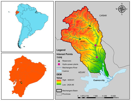
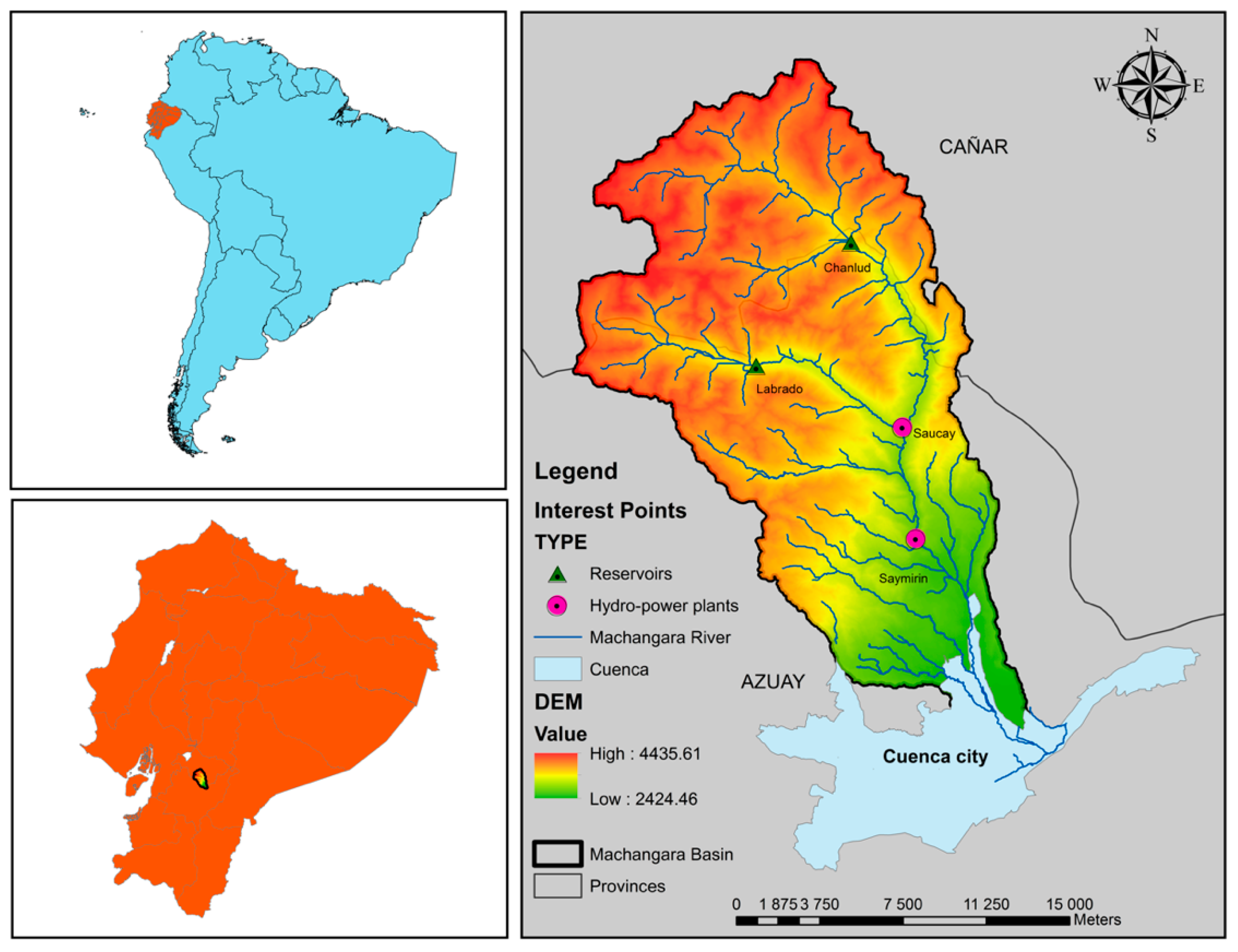
The Machángara River Basin is an Andean basin located in the Azuay and Cañar provinces in southern Ecuador (Figure 1). The total area of the basin is 323.55 km². The Machángara River is an affluent of the Cuenca River and belongs to the hydrographic demarcation of the Santiago River, which is one of the affluents of the Amazon River [6].

Figure 1. The Machángara River Basin in Ecuador.

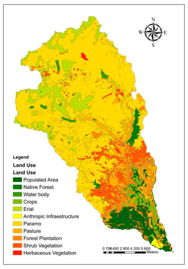
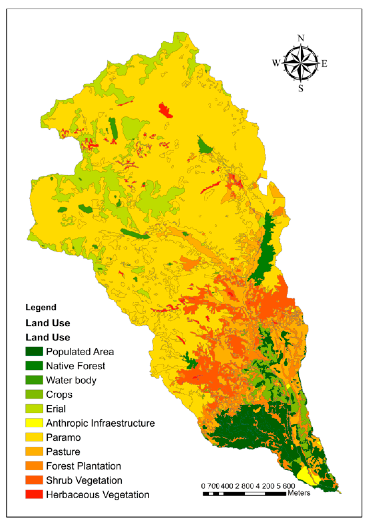
The length of the Machángara River is about 37 km. It crosses the capital of the Azuay province, Cuenca [7]. The altitude in the basin ranges between 2420 masl and 4420 masl with an average of 3420 masl. The land in the basin is used as follows: 6.4% is populated area; 11.3% croplands; 0.5% infrastructures; 59.1% paramo (a treeless vegetation type occurring at higher altitudes); 9.3% pasture; 1.2% native forest; 4.2% forest plantation; 6% shrub vegetation; 1% other herbaceous vegetation, and 1% water body (Figure 2).

Figure 2. Land cover/use distribution of the Machángara Basin.

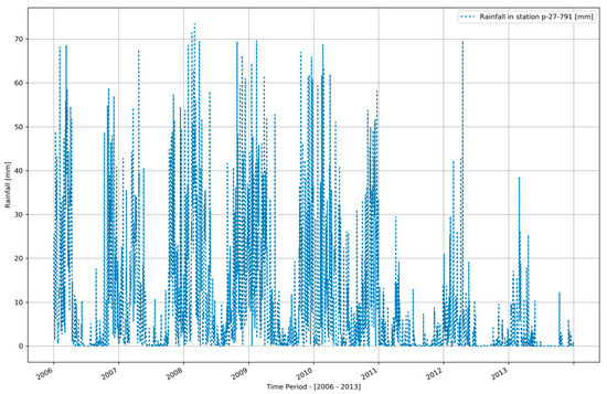
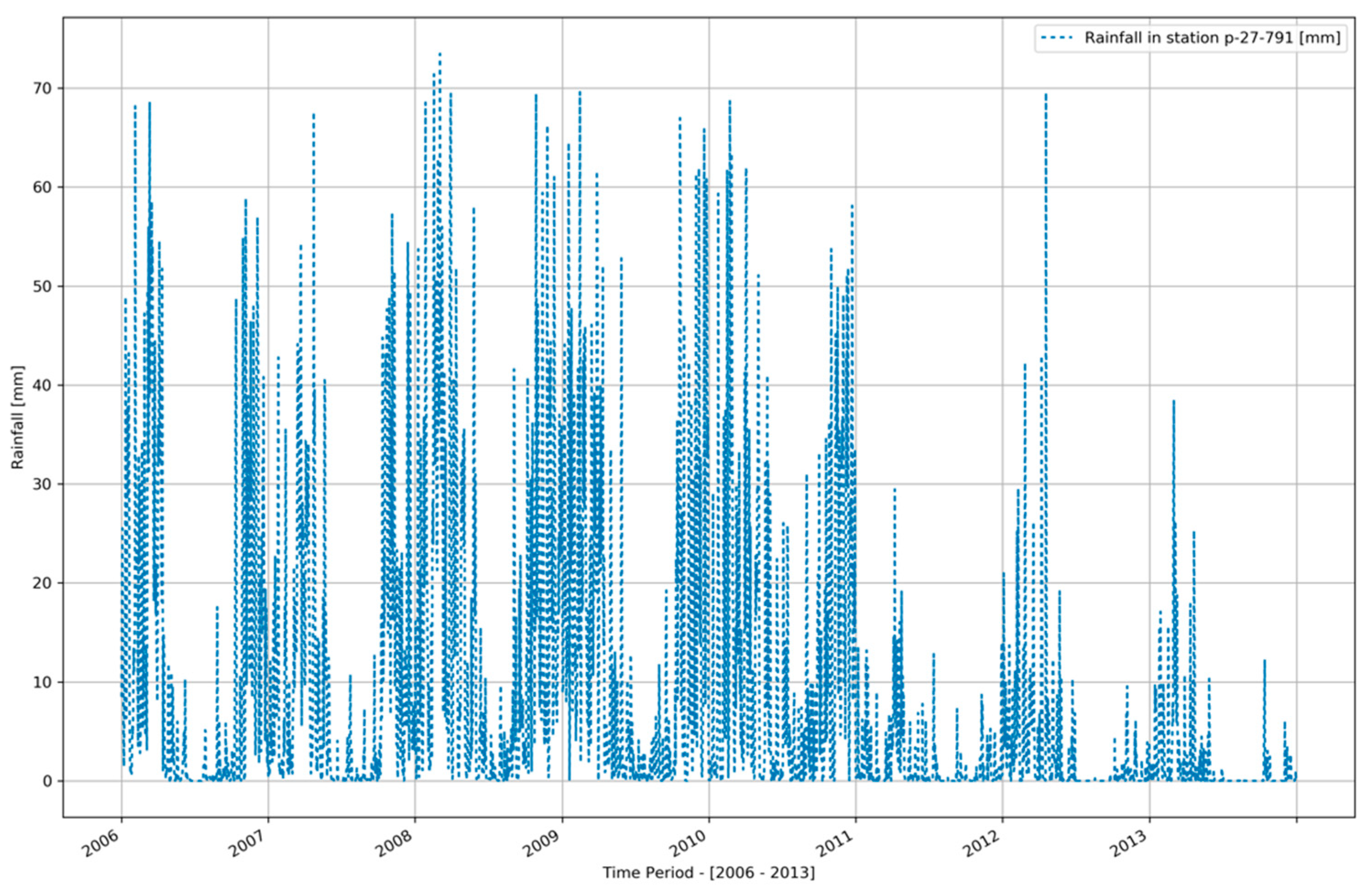
The average annual rainfall depth is 3090 mm of which 2900 mm pertains to the wet season (October–May) and 190 mm to the dry season. However, as it is noticeable from Figure 3, daily rainfall depths reaching 80 mm are not an exception. Besides, at the end of the period (2011–2013), the time series shows that there is less rainfall, which makes the dry season more severe [8].

Figure 3. Daily rainfall observations for the period 2006–2013 in the Machángara Basin. Source: ARCSWAT simulation [9].

2.1.2. Reservoirs, Hydropower Production, and Other Water Uses

The water of the Machángara River is used mainly for domestic and industrial purposes, irrigated agriculture, and hydropower generation. Two reservoirs (Chanlud and Labrado) and two hydro-power plants with reservoirs (Saucay and Saymirin) are located on the Machángara River.

• The Labrado Reservoir is located 40 km north of Cuenca city at 3500 masl. The maximum depth of the reservoir is 13 m and the reservoir’s storage capacity is 6.15 hm³ [10,11,12]. The regulated discharge is 2.4 m³/s [11,12,13].
• The Chanlud Reservoir is located 45 km north of the city of Cuenca. The maximum depth is 51 m and its storage capacity is 17 hm³. The outflow of this reservoir aliments the other two reservoirs (Saucay and Saymirin) as well as the Tixán drinking water treatment plant. This reservoir also aliments several irrigated systems and includes a mechanism to prevent floods [12].
• The Saymirin Reservoir is located in the Chiquintad Parish, 15 km north of Cuenca. It serves the alimentation of several hydropower units with an installed capacity of 7.5 MW [11,12].
• The Saucay Reservoir is located 24 km north of Cuenca. The associated hydropower plant has an installed capacity of 24 MW. Turbines have a maximum discharge of 7.2 m³/s [10,11,12].

The total power generated by the Saucay and Saymirin plants is used to cover the requirements of the provinces of Azuay, Cañar, and Morona Santiago with a total population of 1,085,251 inhabitants [11,14].

In the basin, there is approximately 1300 hectares of irrigated cropland and 133 industrial estates are registered as water users. The drinking water treatment plant “Tixán” treats 600 liters per second to supply water to 140,000 of approximately 810,000 inhabitants of Cuenca city [12].

2.2. Linear Programming Model for Optimising Water Allocation

2.2.1. General

The network flow optimization linear programming model (NFO-LP) [1] is used for the spatiotemporal optimization of the allocation of the water available in the river system to the water demands. The model requires a geometric-topological “arc-node” schematization of the river system, i.e., the network configuration, in which reservoir nodes and transfer nodes are connected by river segments and in which demand segments connect the demand nodes. Reservoir and transfer nodes are characterized by a time series of incoming water while demand nodes are characterized by a time series of water demand. Moreover, reservoirs and segments have minimum and maximum capacities. Trespassing the maximum capacity leads to flooding and a delayed return flow of part of the flooded water to the river. Not reaching the minimum capacity is undesirable for flow continuity and biodiversity considerations. The objective function of the model (Equation (1)) is formulated to release water from the reservoirs and allocate water to the demand nodes to optimally meet the demands, avoid floods, and minimize the under passing of the minimum capacities.

2.2.2. Preliminary River Network Configuration and Water Availability

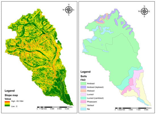
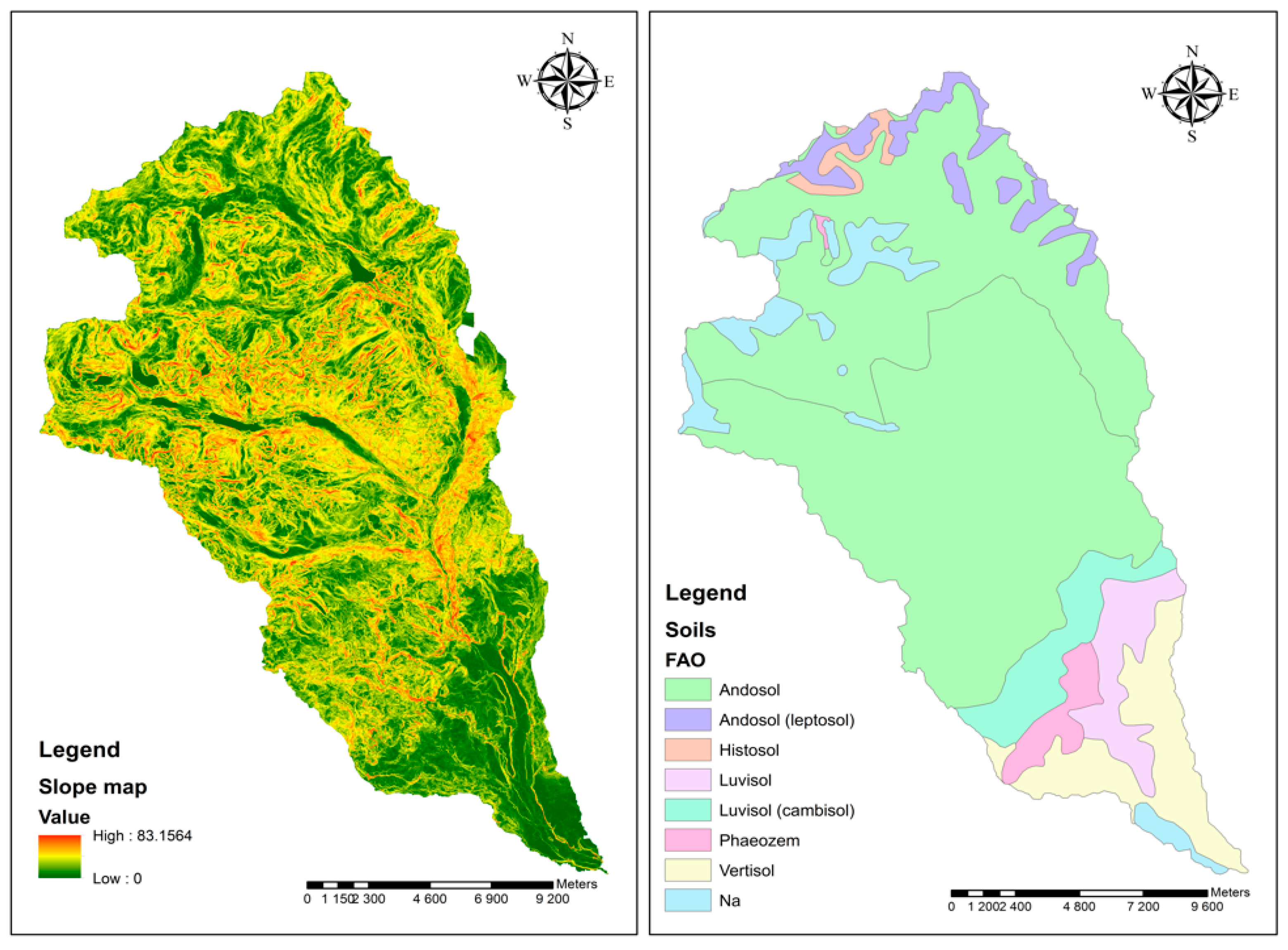
The configuration of the Machángara River network was obtained from a Digital Elevation Model—DEM (resolution = 3 m) using the ArcSWAT-extension of the ArcGIS-software (2012.10.21, University A&M Texas, College Station, TX, USA) [15]. ArcSWAT makes use of the hydrology toolbox of the ArcGIS-software. It extracts the boundaries of a basin and its sub-basins and the flow paths using the flow accumulation algorithm. Transfer nodes are created at the outlet of each sub-basin while reservoir nodes are to be added by the user. To obtain a time series of water inflow in the network through the transfer nodes, a rainfall-runoff simulation using the same ArcGIS-extension was done. To this end, each sub-basin is discretized into so-called hydrological response units (HRU), which are assumed to be homogeneous in terms of slope class, soil type, and land cover type. For each HRU the rainfall-runoff relationship is modeled by assessing the soil water balance in which the runoff is estimated using the curve number method [15]. All water running off from an HRU is assumed to end up in the river system with a time delay. Finally, the inflowing water is propagated through the river segments to reach the outlet eventually. At all nodes, hydrographs are generated by the model. The core of ArcSWAT is the SWAT-tool (Soil and Water Assessment Tool) [15]. SWAT is a semi-distributed model of the land and river phase of the hydrological cycle that quantifies the impact of land management practices on water, sediment, and agricultural chemical yields. SWAT also models physical processes related to water movement, sediment movement, crop growth, etc. Figure 4 displays the DEM-derived slope map and the soil map for the Machángara Basin whereas the DEM and the land use distribution are in Figure 1 and Figure 2 [16]. Daily weather data (rainfall, solar radiation, temperature, relative humidity, and wind direction) were retrieved through the Global Weather Data tool which is accessible at the SWAT-website [9]. For this study area, only one weather station was available. For this station weather data have been generated for the 1979–2014 period by means of the National Centers for Environmental Prediction (NCEP) Climate Forecast System Version 2 (CFSv2, National Centers for Environmental Prediction (NCEP), College Park, MD, USA) [17]. However, only data for 2006–2013 have been effectively used.

Figure 4. Digital slope model (degrees) and the soil map of the Machángara Basin. [16].

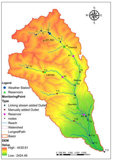
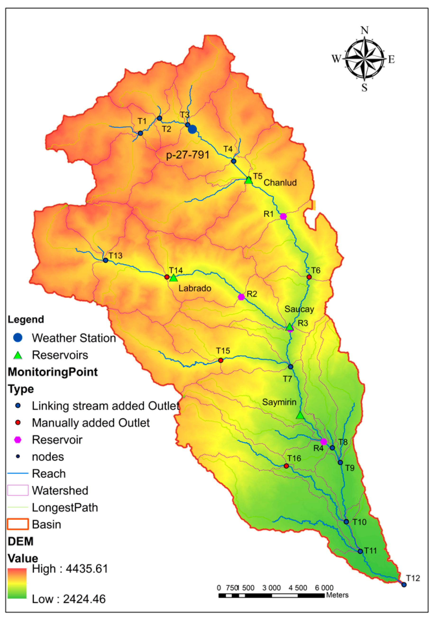
Figure 5 shows the basin subdivision and network configuration generated by ArcSWAT encompassing (a) outlets or transfer nodes (red or blue points), (b) river segments (blue line), and (c) reservoirs (pink point). A transfer node is a location through which water flows from a previous node to the next connected node. A river segment is the portion of the river which connects two nodes. A reservoir node represents a location where a reservoir is installed which can store and release water to the next node. Besides, there is a special kind of node called a “demand node,” which represents the water use in the area.

Figure 5. River network configuration for the Machágara Basin with the location of the virtual weather station.

Each transfer node is identified by a code “Tx” while the code “Rx” is used for reservoir nodes: R1 is Chanlud, R2 is Labrado, R3 is Saucay, and R4 is Saymirin. Additionally, the map includes the location of the virtual weather station “p-27-791” from the Global Weather Data for ArcSWAT [9].

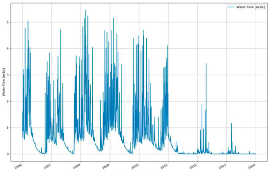
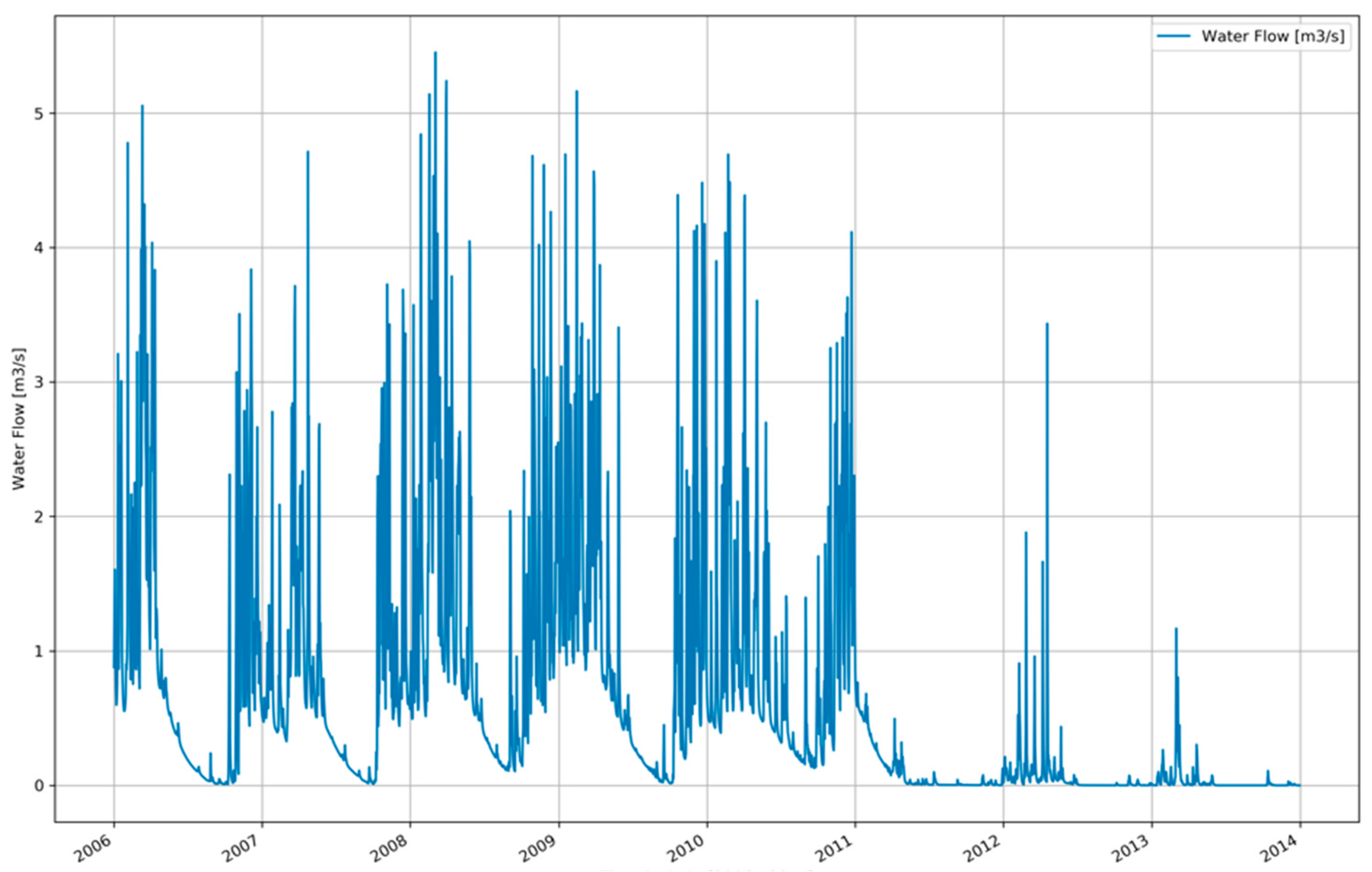
Figure 6 shows the simulated—by means of ArcSWAT—inflow (m³/s) for transfer node T1 over the period 2006–2013. The seasonal rainfall pattern is clearly reflected in the inflow profile.

Figure 6. Simulated water inflow in the Machángara River system at transfer node T1.

2.2.3. Water Demand and Final River Network Configuration

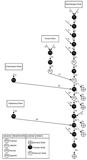
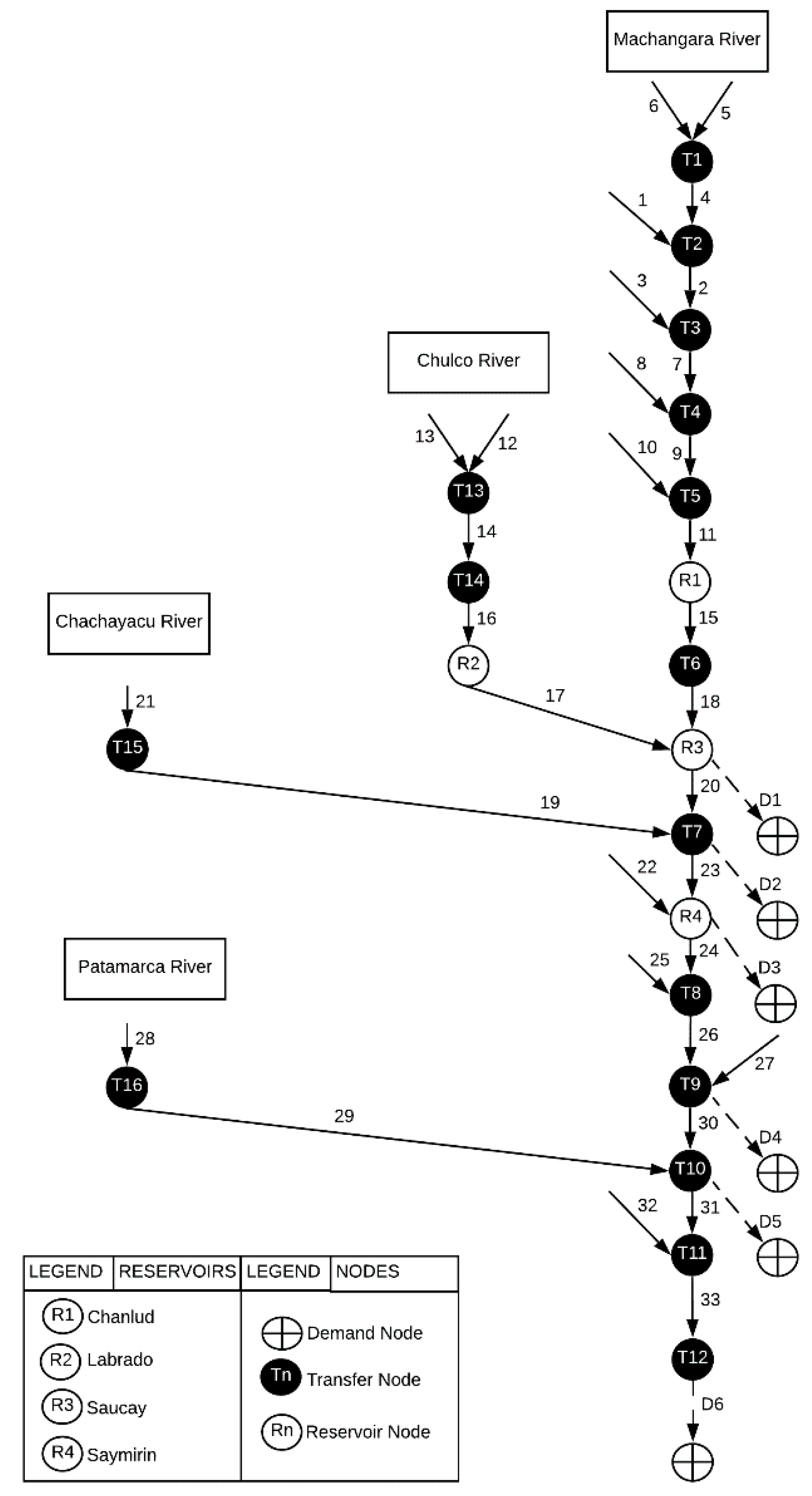
The network configuration resulting from the previous step consists of 16 transfer (T), 4 reservoir (R) nodes and 19 river segments. This preliminary network is to be extended with demand nodes (D) and to be further schematized so that it can be used as a basis for the linear programming model (Figure 7).

Figure 7. The final network configuration of the Machángara River system.

In order to incorporate the water abstraction in the configuration, 6 demand nodes were added. The first one (D1) is associated with the reservoir node “R3” and is characterized by the water needed daily by R3 (Saucay) to generate the required electricity. Water used to generate electricity is assumed to flow back to the river through the next node with a delay of one-time step. The second one (D2) is associated with the water required by the irrigation system “Machángara.” The third one (D3) is associated with the R4 reservoir (Saymirín) and represents the water required by this hydropower plant. The fourth demand (D4) is associated with the drinking water treatment plant “Tixán” and is connected directly with node “T7”. The fifth demand node (D5) represents the water needed by the irrigation system “Sociedad de riego Ricaurte” and it is connected to the node “T10”. The last demand is node D6 which represents the minimum amount of water which needs to flow out of the system in order to preserve its ecological functioning. For the present exercise, the water demands by all six nodes are assumed to be constant through time. The value (hm³/day) is given in Table 1.

Table 1. Daily water demand of the demand nodes [15].

Num.	Demand	Value (hm3 per day)
D1	Sucay powerplant	0.62208
D2	Machangara irrigation project	0.0432
D3	Saymirin powerplant	0.6912
D4	Tixan	0.12096
D5	“Sociedad riego ricaurte”—irrigation	0.02592
D6	Ecosystem	0.01728

Figure 7 shows the final network configuration with the main river (Machángara) and the other three rivers (Chulco, Chachayacu, and Patamarca). The Chulco River is connected to the Machángara River through the reservoirs R2 and R3. The Chachayacu River provides input to the transfer node “T15” and the corresponding segment is connected to the Machángara River with the transfer node “T7.” Finally, the Patamarca River provides input to the “T16” node and is connected through the “T10” node with the Machángara River. It is assumed that water needs one-time step (set to one day in the case study) to flow from one node to the next node.

2.2.4. Objective Function and Constraints

The objective function of the linear programming model to be applied to the established network configuration is the one elaborated in [5,18,19,20] and further explained through Equation (1), while the applicable constraints are expressed with Equations (2)–(23) (Table 2). Indices, parameters, variables and slack variables appearing in the objective function and constraints equations are explained in Table 3.

Table 2. Objective function and constraints from the linear programming (LP)-model.

Description	Constraint
Objective function	$\begin{array}{cc}\hfill \mathrm{minimize}{\displaystyle \sum _n}{\displaystyle \sum _t}({\mathrm{W}}_{\mathrm{n}}& \times {\mathrm{T}}_{\mathrm{n},\mathrm{n}+1}^{\mathrm{t}+})+{\displaystyle \sum _n}{\displaystyle \sum _d}{\displaystyle \sum _t}\left({\mathrm{P}}_{\mathrm{n}}\times {\mathrm{S}}_{\mathrm{n},\mathrm{d}}^{\mathrm{t}-}\right)\hfill \\ & +{\displaystyle \sum _r}{\displaystyle \sum _t}\left(U_r\times S{H}_r^{t-}\right)+ {\displaystyle \sum _r}{\displaystyle \sum _t}\left(A_r\times O{F}_r^{t+}\right)+{\displaystyle \sum _n}{\displaystyle \sum _t}\left(B_n\times Q_{n,n+1}^{t-}\right)\hfill \\ & +{\displaystyle \sum _n}{\displaystyle \sum _d}{\displaystyle \sum _t}\left(E_n\times S_{n,d}^{t+}\right)\hfill \\ & +{\displaystyle \sum _n}{\displaystyle \sum _d}{\displaystyle \sum _t}\left(F_n\times MinX{D}_{n,d}^{t-}\right)+{\displaystyle \sum _n}{\displaystyle \sum _d}{\displaystyle \sum _f}\left(G_n\times MaxX{D}_{n,d}^{t+}\right)\hfill \end{array}$	(1)
Flow balance constraints	Transport (n)
	$\begin{array}{cc}\hfill X_{n-1,n}^t+{\displaystyle \sum }_i{X}_{i,n}^t+{\displaystyle \sum }_r& X_{r,n}^t+V_n^{t-1}+T{D}_{n-2,n-1}^{t-2}+TDF{W}_{n-2,n-1}^{t-2}+R{W}_{n-1,n}^t+O{F}_r^{t+}\hfill \\ & -L_{n-1,n}^t-L_{r,n}^t-L_{n,d}^t+{\displaystyle \sum }_{d}R{D}_{r-2,d-1}^{t-2}\hfill \\ & =V_n^t+L{P}_n^t+X_{n,n+1}^t+{\displaystyle \sum }_r{X}_{n,r}^t+{\displaystyle \sum }_d{X}_{n,d}^t+T{D}_{n,n+1}^t\hfill \end{array}$	(2)
	Reservoir (r)
	${\displaystyle \sum }_n{X}_{n,r}^t+{\displaystyle \sum }_i{X}_{i,r}^t+V_r^{t-1}={\displaystyle \sum }_n{X}_{r,n}^t+V_r^t$	(3)
Network Limitations and capacity constraints	Inputs (i)
	${\displaystyle \sum }_i{X}_{i,n}^t=X_{n,n+1}^t$	(4)
	Sources (i)
	${\displaystyle \sum }_n{X}_{i,n}^t=I_i^t$	(5)
	Demands (d)
	${\displaystyle \sum }_n{X}_{n,d}^t+S_d^{t-}-S_d^{t+}=D_d^t$	(6)
Capacity constraint	River Segments (n)
	$X_{n,n+1}^t+T_{n,n+1}^{t-}-T_{n,n+1}^{t+}=C_{n,n+1max}^t$	(7)
	$X_{n,n+1}^t+Q_{n,n+1}^{t-}-Q_{n,n+1}^{t+}=C_{n,n+1min}^t$	(8)
	Reservoir(r)
	$V_r^t-L{P}_r^t-O{F}_r^{t+}+O{F}_r^{t-}=R_{rmax}^t$	(9)
	$V_r^t-L{P}_r^t+S{H}_r^{t-}-S{H}_r^{t+}=R_{rmin}^t$	(10)
	Demand(d)
	$X_{n,d}^t+MinX{D}_{n,d}^{t-}-MinX{D}_{n,d}^{t+}=C_{n,dmin}^t$	(11)
	$X_{n,d}^t+MaxX{D}_{n,d}^{t-}-MaxX{D}_{n,d}^{t+}=C_{n,dmax}^t$	(12)
Continuity constraint	Continuity constraints
	$V_n^t\le {\beta }_n^t*\left({\displaystyle \sum }_i{X}_{i,n}^{t-1}+{\displaystyle \sum }_r{X}_{r,n}^{t-1}+V_n^{t-1}+X_{n-1,n}^t+R{W}_{n-1,n}^t++TDF{W}_{n-2,n-1}^{t-2}\right)$	(13)
	$V_n^t\ge {\gamma }_n^t*\left({\displaystyle \sum }_i{X}_{i,n}^{t-1}+{\displaystyle \sum }_r{X}_{r,n}^{t-1}+V_n^{t-1}+X_{n-1,n}^t+R{W}_{n-1,n}^t++TDF{W}_{n-2,n-1}^{t-2}\right)$	(14)
Time Delay	All nodes
	$T{D}_n^t={\delta }_n^t\times \left(X_{n,n+1}^t\right)$	(15)
	Flooded Water (n)
	$TDF{W}_{n,n+1}^t={\mu }_n^t\times \left(T_{n,n+1}^{t+}\right)$	(16)
Losses	Transfer nodes (n)
	$L_{n-1,n}^t={\propto }_{n-1,n}^t\times \left(X_{n-1,n}^t\right)$	(17)
	Reservoir nodes (r)
	$L_{r,n}^t={\propto }_{r,n}^t\times \left(X_{r,n}^t\right)$	(18)
	Demand nodes (d)
	$L_{n,d}^t={\propto }_{n,d}^t\ast \left(X_{n,d}^t\right)$	(19)
	Water in Reservoir (r)
	$L{P}_r^t={\theta }_r^t\times \left(V_r^t\right)$	(20)
	Flooded water (n)
	$LF{W}_{n,n+1}^t={\Delta }_{n,n+1}^t\times \left(T_{n,n+1}^{t+}\right)$	(21)
Returning water	Returning water to river segments (n)
	$R{W}_{n,n+1}^t=T_{n,n+1}^{t+}-LF{W}_{n,n+1}^t-TDF{W}_{n,n+1}^t$	(22)
	Water returning from a demand
	$R{D}_{r,d}^t=(1-{\propto }_{r,d}^t)\times \left(X_{r,d}^t\right)$	(23)
	$R{W}_{n,n+1}^t=T_{n,n+1}^{t+}-LF{W}_{n,n+1}^t-TDF{W}_{n,n+1}^t$	(24)

Table 3. Indices, parameters, variables, and slack variables with their assigned value for this case study and some of which are to be calibrated.

Type	Notation	Description	Unit	Value Use Case
Indices	i	input node $\in I$	-	-
	r	reservoir node $\in R$	-	-
	d	demand node $\in D$	-	-
	n	transfer node $\in N$	-	-
	t	time step $\in \mathrm{T}$	-	-
Parameters	$P_d$	Penalty for not meeting the demand with one unit	euro/hm3	1.0 × 106.
	$E_d$	Penalty for exceeding the demand with one unit	euro/hm3	2.0 × 107.
	$F_n$	Penalty for not meeting the minimum river segment capacity with one unit	euro/hm3	5.0 × 106.
	$G_n$	Penalty for exceeding the maximum capacity in a demand segment with one unit	euro/hm3	2.0 ×107.
	$W_n$	Penalty for having a one unit flood in segment (n, n + 1)	euro/hm3	4.0 × 106.
	$B_n$	Penalty not meeting the minimum capacity in segment (n, n + 1) with one unit	euro/hm3	2.0 × 107.
	$U_n$	Penalty for not meeting the minimum capacity of a reservoir with one unit	euro/hm3	8.0 × 106.
	$A_n$	Penalty for exceeding the maximum capacity of a reservoir with one unit	euro/hm3	7.0 × 106.
	${\propto }_{n,n+1}^t$:	Loss factor associated with the river segment (n, n + 1) at time (t)—to be calibrated	-	10%
	${\mu }_{n,n+1}^t$:	Time delay factor associated with the water excess in a river segment (n, n + 1) at time (t) to be calibrated	-	10%
	${\Delta }_{n,n+1}^t$:	Loss factor associated with the water excess in a river segment (n, n + 1) at time (t) to be calibrated	-	10%
	${\beta }_n^t$:	Percentage of water that must flow from the nth node to the next one at time (t), to be calibrated	-	5%
	${\gamma }_{n,}^t$:	Percentage of water that must remain in the nth node until the next time step (t), to be calibrated	-	20%
	${\delta }_{n,n+1}^t$:	Percentage of water that comes to the next node with a time delay in time step (t) to be calibrated	-	10%
	${\mathsf{\theta }}_{\mathrm{r}}^{\mathrm{t}}$:	Loss factor associated to a reservoir to be calibrated	-	10%
	$C_{n,n+1 min}^t$	Minimum capacity of the river segment (n, n + 1) at time (t)	m3	-
	$C_{n,n+1 max}^t$	Maximum capacity of the river segment (n, n + 1) at time (t). The length and width of segment were derived from Google Earth and with a depth of 3m and calculating the cross section [21].	m3	-
	$I_i^t$	Amount of water arriving at the input node (i) at time (t)	m3	-
	$R_{r max}^t$	Maximum capacity of a reservoir -> Table 3	m3	-
	$R_{r min}^t$	Minimum capacity of a reservoir -> Table 3	m3	-
Variables	$V_n^t$	Volume of water in a node (n) at time (t)	m3	-
	${\mathrm{D}}_{\mathrm{d}}^{\mathrm{t}}$	Amount of water needed to meet demand (d) in time (t)	m3	-
	$V_r^t$	Volume of water in the reservoir (r) at time (t)	m3	-
	$X_{n,n+1}^t$	Flow between two nodes, (n) and (n + 1) at time (t) and time (t+1).	m3/day	-
	$X_{r,n}^t$	Flow between a reservoir node (r) and a transfer node (n) at time (t)	m3/day	-
	$X_{n,r}^t$	Flow between a transfer node (n) and a reservoir node (r) at time (t)	m3/day	-
	$X_{i,n}^t$	Flow between an input node (i) and a transfer node (n) at time (t)	m3/day	-
	$X_{i,r}^t$	Flow between an input node (i) and a reservoir node (r) at time (t).	m3/day	-
	$X_{n,d}^t$	Flow between a transfer node (n) and a demand node (d) at time (t)	m3/day	-
	$T{D}_n^t$	Delayed flow from previous nodes and coming into node (n) at time (t).	m3/day	-
	$L_{n,n+1}^t$	Water lost during the flow from transfer node (n) to transfer node (n + 1)	m3	-
	$L_{r,n}^t$	Water lost during the flow from reservoir node (r) to a transfer node (n)	m3	-
	$L_{n,\mathrm{d}}^t$	Water lost during the flow from transfer node (n) to demand node (d)	m3	-
	$L{P}_r^t$	Water lost in a reservoir node (r)	m3	-
	$LF{W}_{n,n+1}^t$	Water lost from the water flooded in the flow process from node (n) to node (n + 1)	m3	-
	$R{W}_{n,n+1}^t$	Water delayed from the water flooded in the flow process from node (n) to node (n + 1)	m3	-
	$R{D}_{r,d}^t$	Water returned from a demand node (d) coming out from a reservoir (r)	m3	-
	$TDF{W}_{n,n+1}^t$	Water delayed from the water flooded in the flow process from node (n) to node (n + 1)	m3	-
Slack Variables	$S_d^{t-}$	Amount of water that cannot be allocated to demand (d) at time (t)	m3	-
	${\mathrm{T}}_{\mathrm{n},\mathrm{n}+1}^{\mathrm{t}+}$	Amount of water above the maximum capacity of node (n) at time (t)	m3	-
	${\mathrm{T}}_{\mathrm{n},\mathrm{n}+1}^{\mathrm{t}-}$	Amount of water under the maximum capacity of node (n) at time (t)	m3	-
	$Q_{n,n+1}^{\mathrm{t}-}$	Amount of water under the minimum capacity of the node (n) at time (t)	m3	-
	$Q_{n, n+1}^{t+}$	Amount of water above the minimum capacity of the node (n) at time (t)	m3	-
	$O{F}_r^{t+}$	Amount of water above the maximum capacity of the reservoir (r) at time (t)	m3	-
	$O{F}_r^{t-}$	Amount of water under the maximum capacity of the reservoir (r) at time (t)	m3	-
	$S{H}_{r }^{t-}$	Amount of water under the minimum capacity of the reservoir (r) at time (t)	m3	-
	$S{H}_{r }^{t+}$	Amount of water above the minimum capacity of the reservoir (r) at time (t)	m3	-
	$MinX{D}_{n,d }^{t-}$	Amount of water under the minimum capacity of the demand river segment (d) at time (t)	m3	-
	$MinX{D}_{n,d }^{t+}$	Amount of water above the minimum capacity of the demand river segment (d) at time (t)	m3	-
	$MaxX{D}_{n,d }^{t-}$	Amount of water under the maximum capacity of the demand river segment (d) at time (t)	m3	-
	$MaxX{D}_{n,d }^{t+}$	Amount of water above the maximum capacity of the demand river segment (d) at time (t)	m3	-

The objective function of the LP model minimizes the total penalty resulting from the water allocation through time to the spatially distributed demand nodes in the network. The total penalty is the result of penalization of the water excess in river segments (floods, T), shortage in river segments (Q), shortages in allocation to demand nodes (S^t−), excess allocation to demand nodes, shortage in reservoirs (SH), overflow in reservoirs (OF), flooding in demand segments (S^t+), shortage in demand segments (MinXD), and overflow in demand segments (MaxXD) whereby each component is associated with a specific penalty value. Equations (2) and (3), model the flow balance constraints; water coming in a node plus the change in water present in the node must equal to the volume of water going out from that node. Equation (2) establishes this constraint for a transfer node, whereas Equation (3) deals with the flow balance of a reservoir node.

Equation (5) specifies the amount of water considered as input to each node. Equation (4) models the water flow to the next connected node and Equation (6) establishes the water supply to a demand node by means of slack variables that allows one to determine the excess as well as the lack of water for meeting the demand.

Equations (7) and (8) set the maximum and minimum capacity of a river segment while Equations (9) and (19) specify the maximum and minimum amount of water to be stored in a reservoir. Equations (11) and (12) set the maximum and minimum capacity of a demand segment.

Equations (13)–(15), represent the continuity constraints. These constraints are associated with both transfer nodes and reservoir nodes. They are meant to keep water moving throughout the water network also in the absence of demands. A maximum and a minimum percentage of water moving from one node to another node are set. Equation (16) determines the fraction of the flooded water that returns to the river with a delay. This delay is established as a percentage of the water passing the node.

Equations (17)–(20) model the fraction of water lost during the transportation process. The water lost with a flood is modeled by Equation (21).

Equation (22) models the amount of flooded water returning to the next node taking the volume of water lost and delayed into account. Equation (23) specifies the amount of water returning from a demand node.

In addition to listing the indices, parameters, variables and slack variables used in the LP-model, Table 3 also displays the penalty values associated to the components of the objective function and the default values to be calibrated.

Reservoirs

In Table 4, the characteristics of the four reservoirs are given: the initial volume of water present, the maximum and minimum volume of water that is allowed and an annual cost associated with the building and management.

Table 4. Reservoir characteristics considered in the LP-model.

Node	Reservoir	Initial Value (hm3)	Maximum Capacity (hm3)	Minimum Capacity (hm3)	Building + Management Cost (Euros per Two Years)
17	R1	5	6.15	1.23	150,000
18	R2	15	16.3	3.26	215,000
19	R3	0.7	1	0.2	100,000
20	R4	0.7	1	0.2	100,000

The building and management cost from Table 4 is computed considering that the total cost of building a reservoir would be around 1.8 × 10⁷ for existing reservoirs (17, 18, 19, and 20 nodes); it is planned that the lifetime of a new reservoir is 240 years [22].

2.3. Extension of the LP-model into a Mixed Integer Linear Programming Model for Locating Reservoirs

2.3.1. General

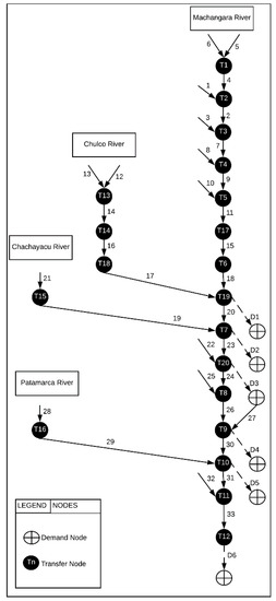
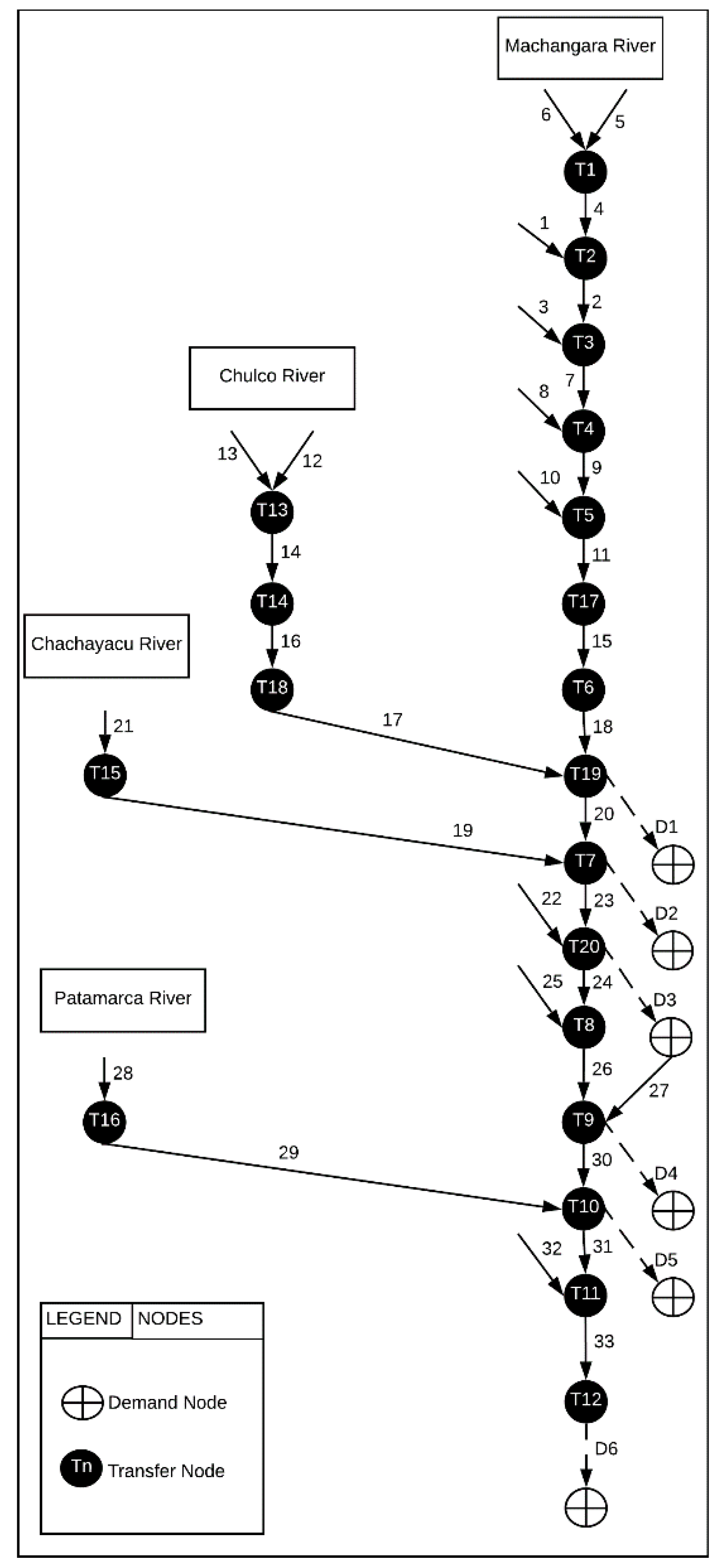
For the MILP-model, each transfer node present in the network configuration (Figure 8) is considered as a potential location for building a new reservoir with a predefined capacity. The model is set up to determine those reservoir locations that keep the sum of costs related to not meeting or exceeding demands or capacities on the one hand and the costs related to the building and management of the reservoirs to a minimum. Hence, the objective function of the previous LP model [5] must be extended with the building and management cost term ($B{C}_n$) for every possible reservoir ($Y_n$). $Y_n$ is a binary variable indicating whether location n has or has not been selected.

Figure 8. The final network configuration of the Machángara River system as to the MILP model.

2.3.2. Candidate Reservoirs and Capacity

All 16 candidate reservoirs are assumed to (i) have a maximum capacity of 13 hm³, (ii) store at least 1.3 hm³ (nodes 1, 2, and 3) and 2 hm³ (nodes from 4 to 16) of water, (iii) store an initial water volume of 2.6 hm³ and have an annual depreciation of the building and management cost of 195,000 euros per two years.

2.3.3. Objective Function and Constraints

Objective Function

$$\begin{array}{cc}\hfill \mathrm{minimize}{\displaystyle \sum _n}{\displaystyle \sum _t}(W_n& \times T_{n,n+1}^{t+})+{\displaystyle \sum _n}{\displaystyle \sum _d}{\displaystyle \sum _t}\left(P_n\times S_{n,d}^{t-}\right)+{\displaystyle \sum _r}{\displaystyle \sum _t}\left(U_r\times S{H}_r^{t-}\right)+ {\displaystyle \sum _r}{\displaystyle \sum _t}\left(A_r\times O{F}_r^{t+}\right)\hfill \\ & +{\displaystyle \sum _n}{\displaystyle \sum _t}\left(B_n\times Q_{n,n+1}^{t-}\right)+{\displaystyle \sum _n}{\displaystyle \sum _d}{\displaystyle \sum _t}\left({\mathrm{E}}_{\mathrm{n}}\times {\mathrm{S}}_{\mathrm{n},\mathrm{d}}^{\mathrm{t}+}\right)\hfill \\ & +{\displaystyle \sum _n}{\displaystyle \sum _d}{\displaystyle \sum _t}\left(F_n\times MinX{D}_{n,d}^{t-}\right)+ {\displaystyle \sum _n}{\displaystyle \sum _d}{\displaystyle \sum _f}\left(G_n\times MaxX{D}_{n,d}^{t+}\right)+{\displaystyle \sum }\left({\mathrm{BC}}_{\mathrm{n}}\times {\mathrm{Y}}_n\right)\hfill \end{array}$$

(25)

In order to consider a candidate reservoir for selection, its characteristics such as maximum and minimum capacities must be considered. This is done by updating the reservoir capacity constraints from the LP-model (Equations (9) and (10)) according to Equations (25) and (26). To specify the minimum number of the reservoirs to be selected, Equation (27) is added. No changes are required in the flow balance constraints, capacity constraints, continuity constraints, or time delay constraints as formulated for the LP-model (Table 2)

Capacity Constraints

(a) Reservoir(s)

$$V_r^t-L{P}_r^t-O{F}_r^{t+}+O{F}_r^{t-}<=R_{r max}^t+M_r\times \left(1-Y_r\right)$$

(26)

$$V_r^t-L{P}_r^t+S{H}_r^{t-}-S{H}_r^{t+}>=R_{r min}^t-M_r\times \left(1-Y_r\right)$$

(27)

(b) Number of reservoirs

$${{\displaystyle \sum }}_{\mathrm{i}}{Y}_i\ge 1$$

(28)

3. Results

3.1. Calibration and Validation of LP-Model

Seven parameters of the LP-model listed in Table 2 need calibration for the model to reproduce reality as closely as possible. Since no observed data on water availability and flow in the river systems was available, the water flow in the nodes of the river configuration computed by the ArcSWAT-tool in the absence of demands was taken as a proxy for reality. The first four years (2006–2009) of the studied 2006–2013 period were used for calibration. For a usable calibration, the LP-model was used in simulation rather than the optimization mode. This was done by setting the water demands to zero.

3.1.1. Calibration

The seven parameters in the LP model which require calibration are ${\propto }_{n,n+1}^t$; ${\Delta }_{n,n+1}^t$:; ${\theta }_r^t$:; ${\delta }_{n,n+1}^t$:; ${\mu }_{n,n+1}^t$:; ${\beta }_n^t$: and ${\gamma }_{n,}^t$: (Table 3). All these parameters are fractions ranging from 0 to 1.

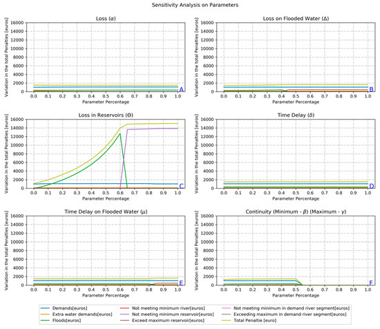
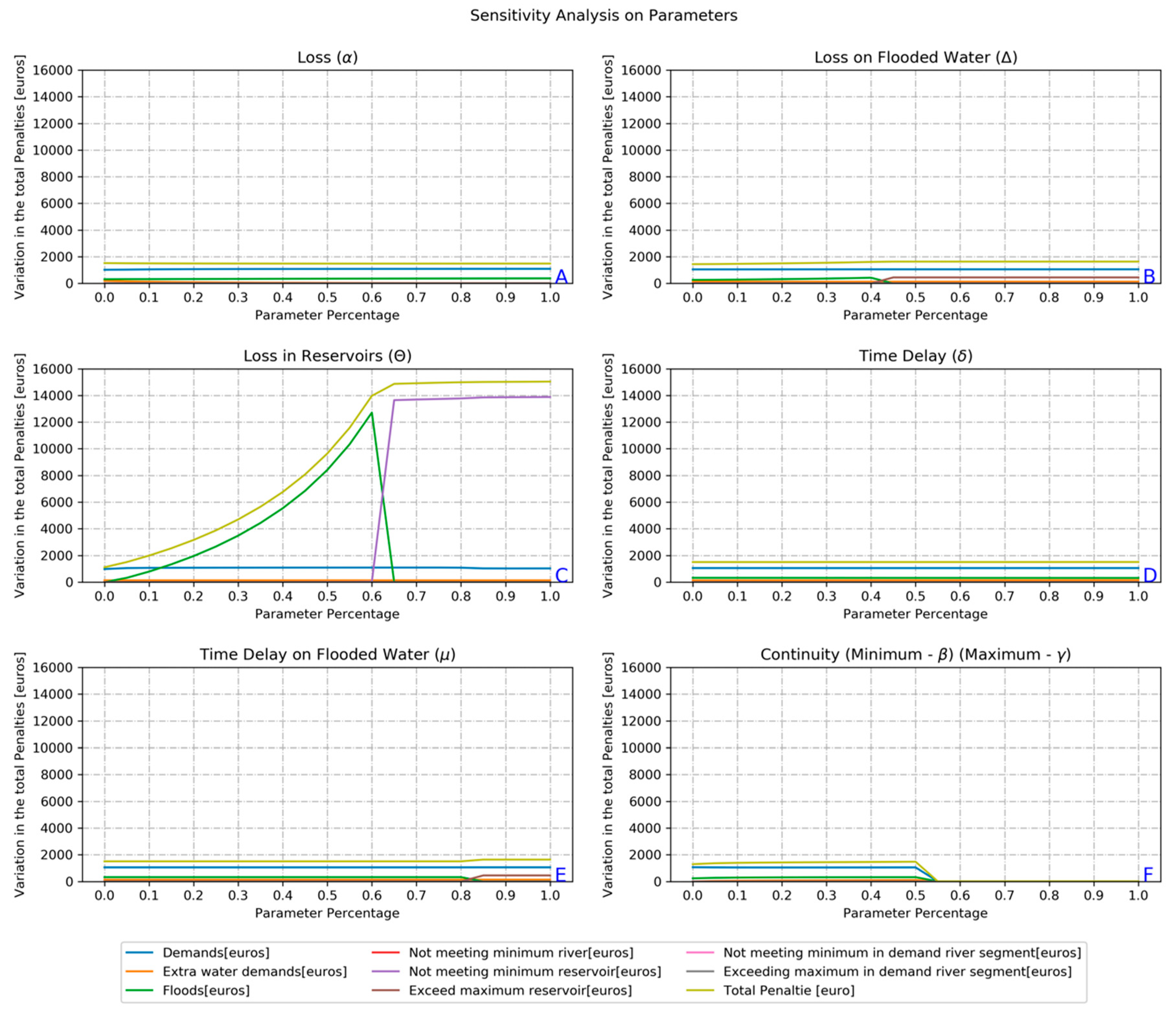
First, a sensitivity analysis was carried out. One parameter at a time was iteratively changed from 0 to 1 with a step of 0.05. The model was run, and the component and total penalties computed. Charts A to F in Figure 9 displays the results of this univariate sensitivity analysis. For two parameters, i.c. the minimum and maximum fractions of water present in a node that must remain in the node ($\beta$) ($\gamma$). There is only one chart (F) since beta ($\beta$) must always be smaller than gamma ($\gamma$) to avoid the model becoming infeasible. Figure 9 shows that parameter $\theta$ (loss factor in reservoirs) is the most sensitive one.

Figure 9. The sensitivity of the LP-model parameters.

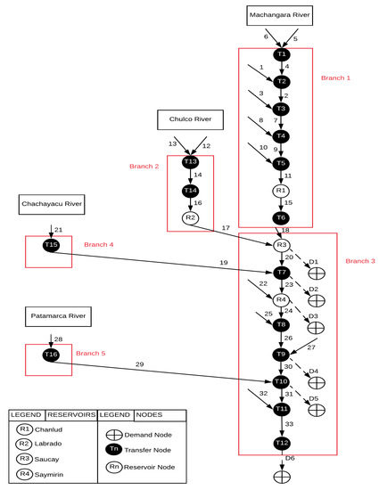
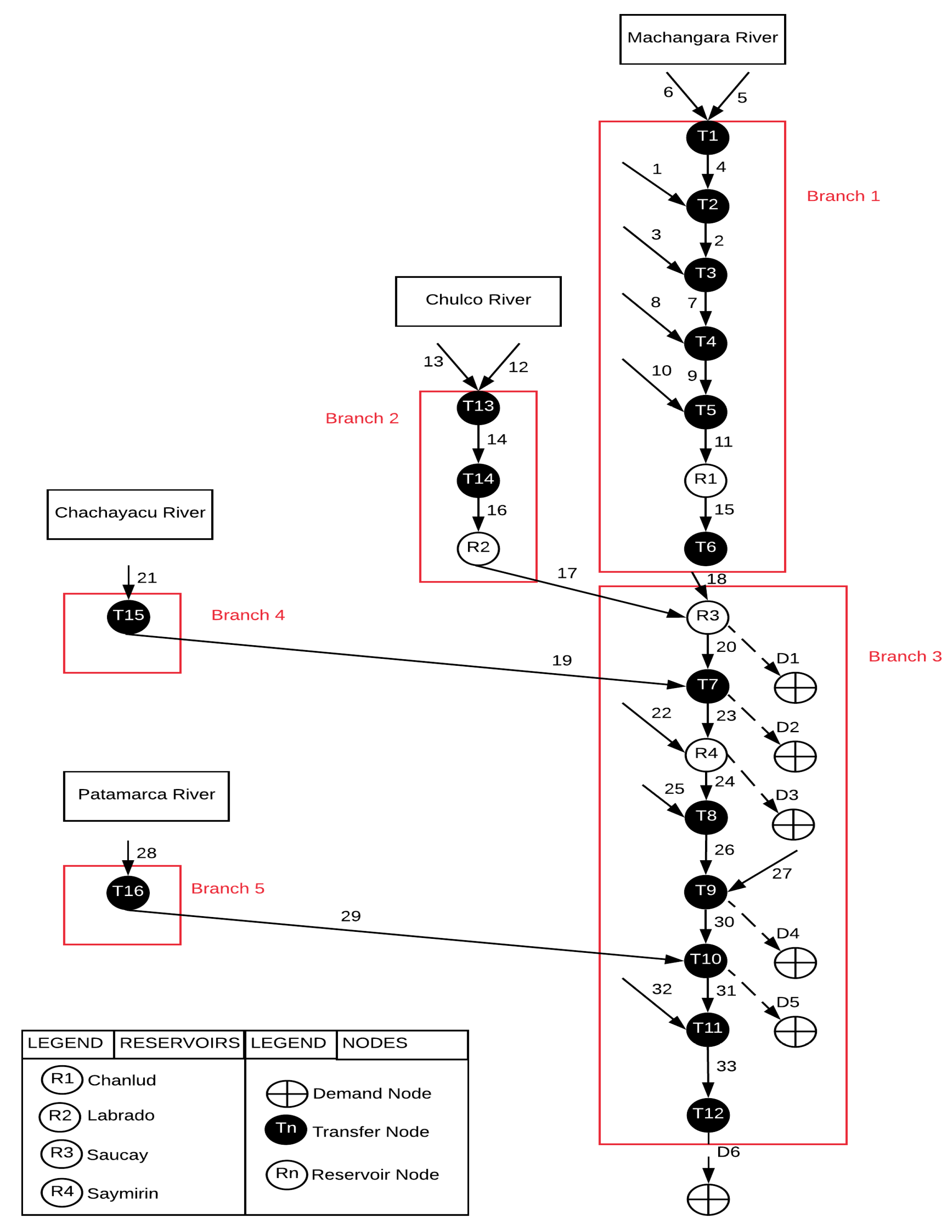
The calibration consisted of an iterative trial and error procedure in which the most sensitive parameters were adjusted in order to minimize the difference between the total penalty value obtained from the LP model and the reference value generated by the ArcSWAT model. The adjustment was not done for each of the 19 segments but rather for each of the five branches of the river system as depicted in Figure 10.

Figure 10. River network branches used for calibration of the parameters of the LP-model.

The initial values of the six node-/segment-related parameters for each of the five branches are between 0 and 1. Therefore, Table 5 shows the calibrated values of the parameters of the LP model per segment and per branch. The root mean square error (RMSE) and the relative root mean square error (RRMSE) are used to evaluate the performance of the LP-model. These two types of indicators will allow one to compute the deviation of the LP-model and the referential model (ArcSWAT). Moreover, the total RRMSE reaches a total of 103%.

Table 5. Parameters per segment during the final iteration.

Branch	$\mathbf{Loss}(\propto )$	Loss Flooded Water (∆)	$\mathbf{Time}\mathbf{Delays}\left(\mathit{\delta }\right)$	Time Delay Flooded Water (μ)	$\mathbf{Minimum}\mathbf{Water}\mathbf{to}\mathbf{Stay}\left(\mathit{\gamma }\right)$	$\mathbf{Maximum}\mathbf{to}\mathbf{Stay}\left(\mathit{\beta }\right)$	$\mathbf{Loss}\mathbf{in}\mathbf{Reservoirs}\left(\mathit{\theta }\right)$
1	1.0 × 10−5	0.2	1.0 × 10−5	0.001	0.001	0.002	0.01
2	1.0 × 10−5	0.2	1.0 × 10−5	0.001	0.001	0.002	0.01
3	1.0 × 10−9	0.2	1.0 × 10−9	0.001	0.001	0.002	0.01
4	1.0 × 10−5	0.2	1.0 × 10−5	0.001	0.001	0.002	0.01
5	1.0 × 10−5	0.2	1.0 × 10−5	0.001	0.001	0.002	0.01

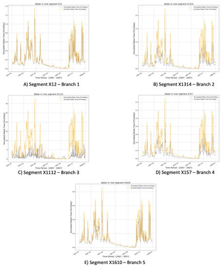
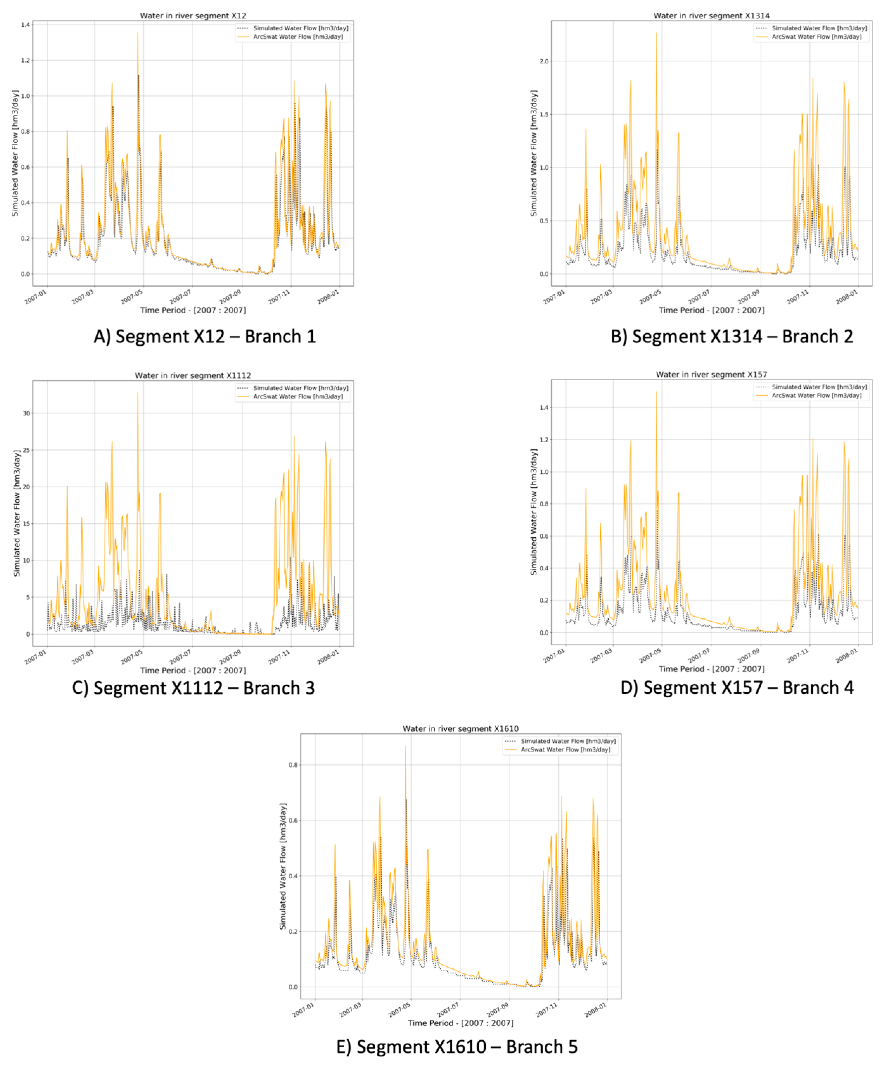
Charts in Figure 11 show the water flowing in one segment of each considered branch as simulated by the LP-model on the one hand and the ArcSWAT-model on the other hand. Only a one-year period (2007) is displayed to reduce the size of the chart and make clearer the comparison with the outputs of both models. Chart A shows river segment X12 from branch 1 while chart E shows segment X1610 part of branch 5. In both segments, there is a close agreement between the LP-modelling results and the reference data. In chart B (branch 2), D (branch 4), and C (branch 3) the deviations are larger, but the temporal patterns are in acceptable agreement.

Figure 11. The comparison of the water flow as simulated by the calibrated LP-model and the ArcSWAT-reference.

3.1.2. Validation

Validation of the parameterized LP-model was done by comparing its output with the ArcSWAT time series for the 2010–2011-period. Thus, the initial values of each node with the model are the outputs of the model during the calibration process (2006–2009 dataset). The values of the parameters are the ones shown in Table 5.

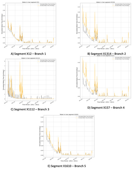
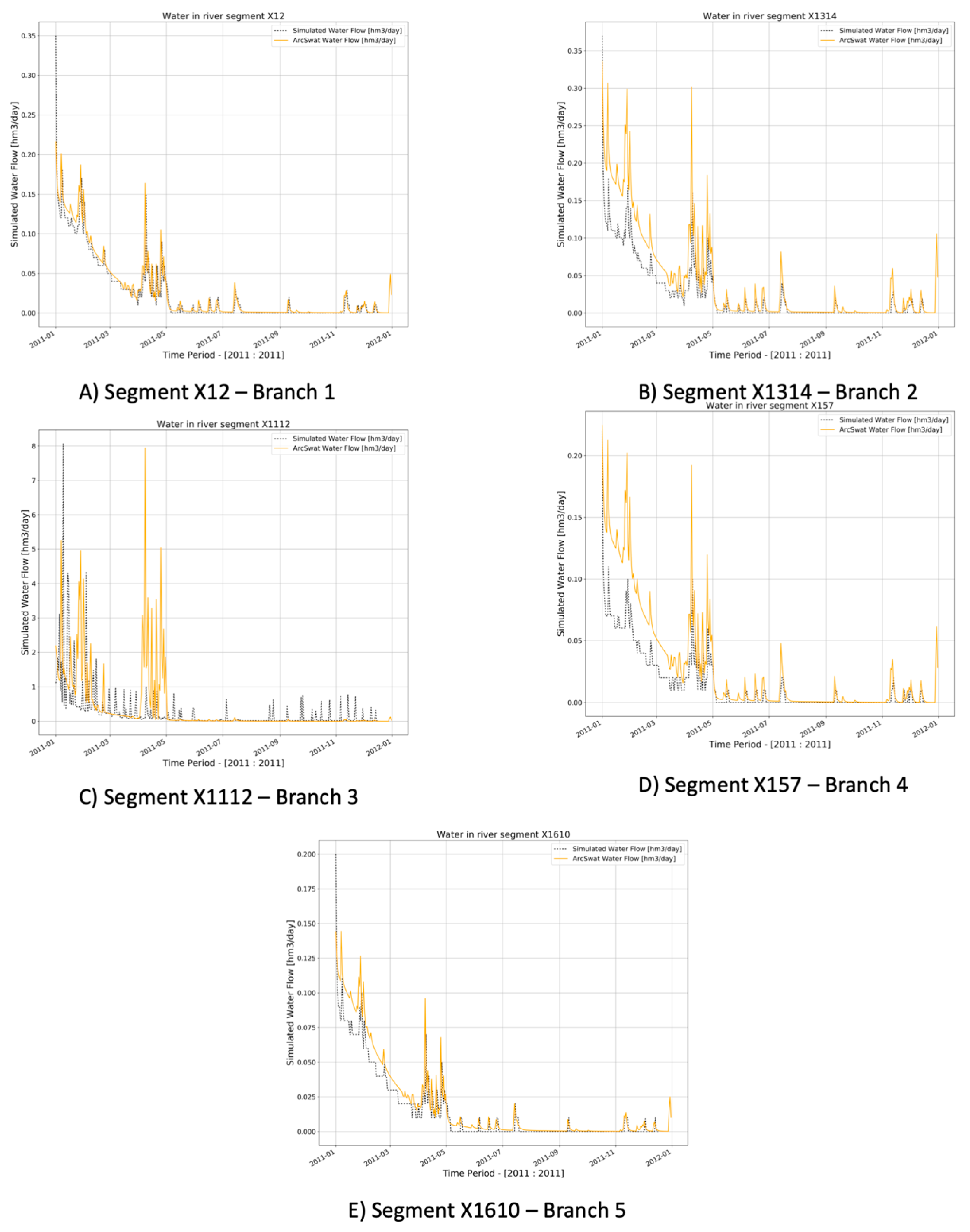
In Figure 12 (only one year from the original dataset), five charts are included all of which have a counterpart in Figure 11. The purpose of the validation process was to verify whether the values of the parameter obtained from the calibration process apply to a different dataset. From the charts, it can be observed that the ArcSAT reference pattern is largely reproduced by the calibrated LP-model but that peaks are underestimated. The latter is also reflected in the relatively high RRMSE of 137%.

Figure 12. Comparison of the water volume present within the river segments as computed by ArcSWAT with the volumes simulated by the calibrated LP model for the 2010–2011 period.

3.2. Application of the Calibrated and Validated LP-model

Finally the calibrated and validated LP-model was applied for the 2012–2013 period (using 2010–2011 outputs to initialize the model) to optimally allocate the available water to the demand nodes (Figure 7) considering their daily demands for water (Table 1) and the unit penalty values of not meeting or exceeding these demands and the penalties related to the river segments ($\propto$, $\Delta$, $\delta$, $\mu$, $\beta$, and $\gamma$), the reservoirs ($\theta$), and the demand segments ($\propto$, $\Delta$, $\delta$, and $\mu$) (Table 3).

3.2.1. Linear Programming Model

Water in Reservoirs

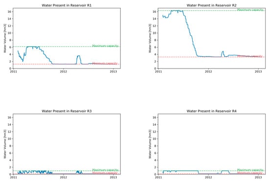
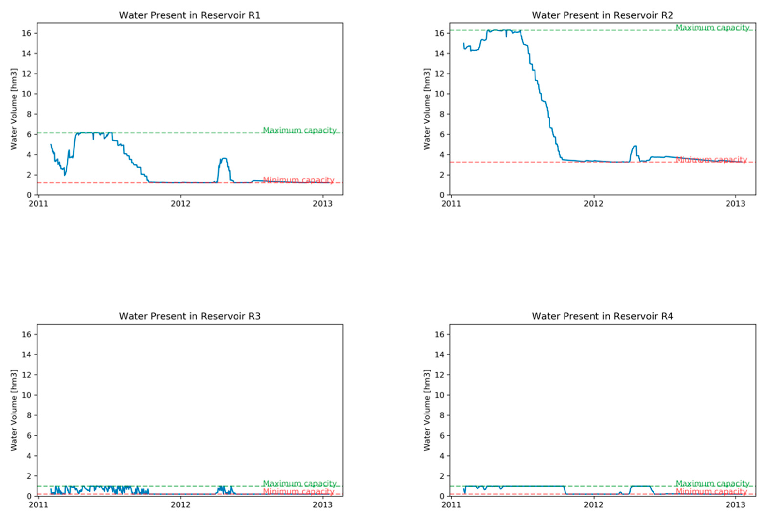
Figure 13, shows the total amount of water stored in each of the four reservoirs during the considered 2-year period. In reservoir R1 (Node 17), one can see the seasonal rainfall pattern and water levels are always between the maximum and minimum capacities. This reservoir is located upstream in the main river “Machangara.” Also, reservoir R2 (node 18) is located upstream but on the “Chulco” river basin. Despite the optimization of the water allocation, this reservoir is gradually exhausted. Reservoirs R3 (node 19) and R4 (node 20) are located more downstream in the river system and receive water from tributaries and the regulated, through the upstream reservoirs, the main river which masks the seasonal rainfall pattern. From Figure 13, the maximum and minimum capacities are shown in dashed lines: maximum (green line) and minimum (red line).

Figure 13. Water stored in reservoirs.

Penalties

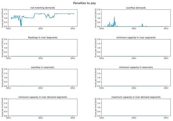
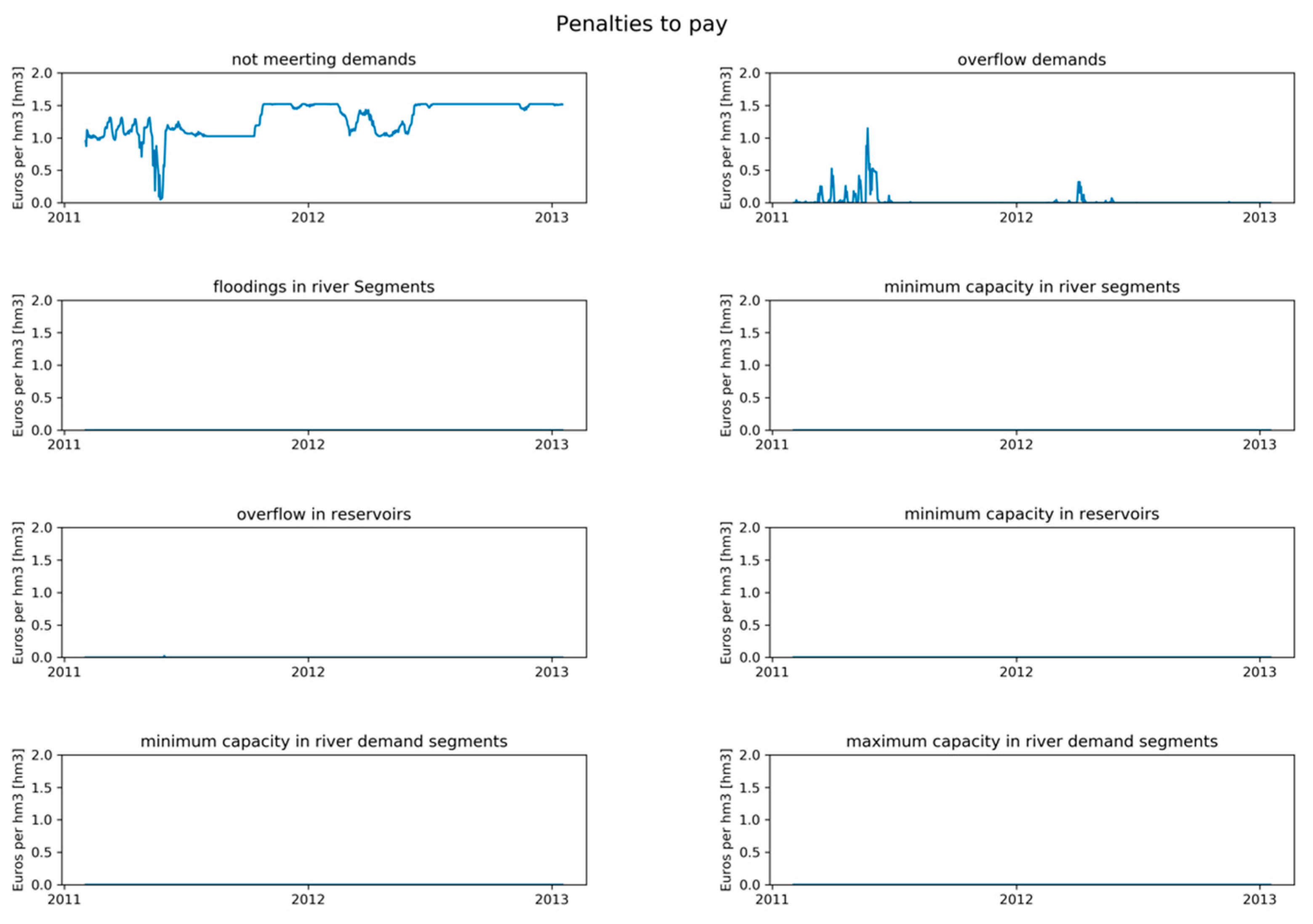
From Table 6 and Figure 14, it is clear to see that the major terms in the total penalty are the delivery of too little water to the demand nodes starting in the second half of the 2-year period and the delivery of too much water in the first six months of the period. This behavior represents the seasonal pattern of rainfall distribution.

Table 6. Deviation between the volume of water targeted and achieved after optimization (m³) and associated penalties (€).

Penalties (Euros)	Value (Euros)	Values (Euro/hm3)
(a) Penalty for not meeting the demands	920.81	920.81
(b) Penalty for exceeding the demands	3.44 × 108	17.17
(c) Penalty flooding of river segments	0.00	0.00
(d) Penalty for not meeting the minimum capacity in the river segments	0.00	0.00
(e) Penalty for exceeding the maximum capacity in reservoirs	1.82 × 105	0.03
(f) Penalty for not reaching the minimum capacity in reservoirs	0.00	0.00
(g) Penalty for not reaching the minimum capacity in demand segments	0.00	0.00
(h) Penalty for exceeding the maximum capacity in demand segments	0.00	0.00
(i) Building + management cost	5.65 × 105	0.00
Total (a) + (b) + (c) + (d) + (e) + (f) + (g) + (h) + (i)	3.45 × 108	938.01

Figure 14. Daily penalties during the 2-year period.

3.3. Application of the MILP-Model

Mixed Integer Linear Programming Model

From Table 7, several statements can be made. The results of the LP model are considered as the base model and this model includes four reservoirs (17, 18, 19, and 20), and is associated with a total penalty of 3.45 × 10⁸ euros. Thus, the MILP-model, as well as the LP-model, try to reduce the total penalty; from the objective function, it is noticeable that several components can result in paying penalties, so those components are considered as boundaries; if the results of the execution of the model cross those boundaries, a penalty value must be paid. Besides, the use of a specific reservoir would result in adding an extra cost (building and management cost). Therefore, the main objective is to select a new reservoir based on the minimization of costs as well as to recommend where to build a reservoir in order to reduce penalties. There are several executions of the MILP model, iterating over the number of the reservoirs included in the solution. Table 7, shows that as more reservoirs are included, the total water not allocated is reduced. Moreover, from the execution of use case 6, the total water not allocated is reduced by using 5 reservoirs: 10, 12, 17, 19, and 20. After, as many reservoir are included in the possible solution, more water is being allocated to the demand nodes; for this particular case, it is also clear that from the existing reservoirs from the LP-model only the reservoir 18 is not in the solution. Furthermore, with the execution of the use of case 2 (one reservoir), the MILP model is not able to allocate water to all the demands without incurring other types of penalties from Table 3.

Table 7. Summary of the results of including a different number of reservoirs in the MILP model.

Use Case	Number of Reservoirs	Reservoirs Included in the Solution		Water Not Allocated	Penalties (Euros)	Building + Management (Euros)	Total
1	0	-		934.975	1.97 × 108	0.00	1.97 × 108
2	1	12		926.707	9.27 × 108	1.95 × 105	9.27 × 108
3	2	12,20		926.39	9.26 × 108	2.95 × 105	9.27 × 108
4	3	12,19,20		925.429	9.25 × 108	3.95 × 105	9.26 × 108
5	4	11,13,19,20		925.094	9.25 × 108	5.90 × 105	9.26 × 108
6	5	10,12,17,19,20		916.215	9.16 × 108	7.40 × 105	9.17 × 108
7	6	9,10,12,17,19,20		911.807	9.12 × 108	9.35 × 105	9.13 × 108
8	7	9,10,12,13,17,19,20		911.329	9.11 × 108	1.13 × 106	9.12 × 108
9	8	9,10,12,13,14,17,19,20		910.859	9.11 × 108	1.33 × 106	9.12 × 108
10	9	9,10,12,13,14,15,17,19,20		910.315	9.10 × 108	1.52 × 106	9.12 × 108
11	10	8,9,10,12,13,14,15,17,19,20		908.859	9.09 × 108	1.72 × 106	9.11 × 108
12	11	7,8,9,10,12,13,14,15,17,19,20		908.438	9.08 × 108	1.91 × 106	9.10 × 108
13	12	7,8,9,10,12,13,14,15,16,17,19,20		908.38	9.08 × 108	2.11 × 106	9.10 × 108
14	13	7,8,9,10,11,12,13,14,15,16,17,19,20		908.324	9.08 × 108	2.30 × 106	9.11 × 108
15	14	6,7,8,9,10,11,12,13,14,15,16,17,19,20		907.759	9.08 × 108	2.50 × 106	9.10 × 108
16	15	5,6,7,8,9,10,11,12,13,14,15,16,17,19,20		907.267	9.07 × 108	2.69 × 106	9.10 × 108
17	16	4,5,6,7,8,9,10,11,12,13,14,15,16,17,19,20		906.703	9.07 × 108	2.89 × 106	9.10 × 108
18	17	3,4,5,6,7,8,9,10,11,12,13,14,15,16,17,19,20		906.212	9.06 × 108	3.08 × 106	9.09 × 108
19	18	2,3,4,5,6,7,8,9,10,11,12,13,14,15,16,17,19,20		905.701	9.06 × 108	3.28 × 106	9.09 × 108
20	19	1,2,3,4,5,6,7,8,9,10,11,12,13,14,15,16,17,19,20		905.166	9.05 × 108	3.47 × 106	9.09 × 108
21	20	1,2,3,4,5,6,7,8,9,10,11,12,13,14,15,16,17,18,19,20		872.398	8.72 × 108	3.69 × 106	8.76 x108

4. Discussion

Although no real-world data are available about how well the demands for water in the Machángara Basin were met in the 2012–2013 period, this study shows that also after optimization, using our LP-model, of the allocation of the available water to the spatially distributed demand nodes with constant temporal demands, not all demands can be met at all times. Hence a nexus is present and will remain present between the availability of water and the demands for hydropower production, irrigated agriculture, and domestic and industrial use because these demands are expected to increase with the growth of the population and its welfare aspirations. The construction of one or more new reservoirs will mitigate the nexus but it will be far from eliminating all the shortages and undesired phenomena like floods and excess supply. Given the low return on investment of one or more new reservoirs, it seems best not to build new ones but to optimize the use of the existing reservoirs. Particular attention in our (MI)LP-models is needed for the calibration of seven empirical parameters expressing the losses of water from segments, reservoirs, and floods, temporal delays of flooded water and water used for hydropower production to return to the river system and factors needed to model the continuous flow of water through a river system, even in the absence of demands. Through a trial and error calibration procedure, we succeeded in modeling the reference water flow dynamics in the river system with an acceptable accuracy although peak discharges were underestimated. Mixed integer linear programming models, like in this paper, should be considered as a decision point when there are several possibilities to build a new reservoir. A MILP model allows us to recommend possible locations for new reservoirs and also to simulate the current configuration in a river network. However, the values used as a building and management cost are only estimated and might be improved by using values closer to reality. One of the advantages of the MILP model is that the building cost might be removed for the objective function and then several scenarios can be performed considering only the water allocation principal. Therefore, stakeholders should have several options as solutions.

As for any model, the quality of the input data and the quantification of the initial situation is crucial for our (MI)LP-models. In this study, we had to rely on water inputs in the system as simulated by the well-established SWAT-model using the default model parameter values, from the time series of meteorological data provided by NECP Climate Forecast System Version 2, which have no observed time series. This input and reference output data allowed us to show and discuss our (MI)LP modeling approach, but for real-world application of our (MI)LP-models, they must be substituted by observed meteorological time series and observed river discharge measurements, meaning that for the calibration and validation phase data about effective water abstraction and the possible return of water to the river systems must be taken into account.

5. Conclusions

Compared to physically based models which are routinely used to study the impacts of changing meteorological, hydrological, infrastructural, and demand conditions on the availability in space and time of water in a given river system [23,24,25], from the simulation perspective, our LP-model is a simple one. It uses only a few parameters to model the temporal dynamics and loss of water coming into the river system assuming that the time needed for water released in one node to flow to the next is always one time step. Furthermore, water supply networks (WSN), such as in this study, can be extended to include new components (more nodes, water demand users, etc.) to create a network closer to reality. In this way, several issues might become part of these networks. Therefore, a procedure to verify the risk, and assess and validate the applicability and usability of the new WSN must be included, such as in the research from Pietrucha-Urbanik and Tchorzewska-Cieslak [26].

The strength of our LP-model, however, is not based on the sophistication of the simulation of water retention and flow but its capability to optimize the allocation of the available water to spatially distributed demand nodes, also considering temporal variability of the demand (not done in this study). Few other models have been reported in the literature which were developed for this purpose; Hu et al. and Labadie [27,28] state that optimization in the water allocation process is possible. There are several hydrological models based on differential equations which can model the behavior of a river basin [29] and even allocate water [23,24,25]. However, those models are not capable of optimizing the water allocation. Moreover, by using this mathematical approach (linear programming and mixed integer linear programming) it is possible to get an optimal solution among the several feasible solutions that can exist. Moreover, a straightforward extension of the conceptual LP-approach is to consider all or a subset of nodes in the river network as candidate (Yes/No) locations for a reservoir with predefined storage capacity. Consequently, we have addressed this extension by adding a term with a binary variable in the objective function of the LP-model, generating a MILP-model that can select the most appropriate locations for new reservoirs with a few to optimize the water allocation further while taking investment and management costs into account.

To extend the work presented in this paper, as well as to validate the LP-model and the MILP-model, it is planned to extend the LP-model to deal with changes in capacity within reservoirs. Thus, the sedimentation phenomenon will be taken into account and modeled. Additionally, an extra effort is planned to validate both models (LP and MILP) in two different study areas: Omo–Turkana River Basin, located in the central-east part of Africa; this basin is surrounded by four countries: Ethiopia, Kenya, Uganda, and Sudan; and the Lunsemfwa River Basin located in Zambia, the central and southern part of Africa.

References

- Sharma, B.; Neupane, N.; Amjath-Babu, T.S.; Wahid, S.M.; Sieber, S.; Rasul, G.; Bhattarai, U.; Brouwer, R. Integrated modelling of the impacts of hydropower projects on the water-food-energy nexus in a transboundary Himalayan river basin. Appl. Energy 2019, 239, 494–503. [Google Scholar]
- Liu, P.; Zou, H.; Guo, S.; Zeng, Y.; Shen, Y.; Liu, D.; Zhang, J.; Xiong, L.; Tian, J. Optimisation of water-energy nexus based on its diagram in cascade reservoir system. J. Hydrol. 2018, 569, 347–358. [Google Scholar] [CrossRef] [Scilit]
- Allam, M.M.; Eltahir, E.A.B. Water-Energy-Food Nexus Sustainability in the Upper Blue Nile (UBN) Basin. Front. Environ. Sci. 2019, 7. [Google Scholar] [CrossRef] [Scilit]
- Zeng, X.T.; Zhang, J.L.; Yu, L.; Zhu, J.X.; Li, Z.; Tang, L. A sustainable water-food-energy plan to confront climatic and socioeconomic changes using simulation-optimization approach. Appl. Energy 2019, 236, 743–759. [Google Scholar] [CrossRef] [Scilit]
- Veintimilla-Reyes, J.; De Meyer, A.; Cattrysse, D.; Van Orshoven, J. A linear programming approach to optimise the management of water in dammed river systems for meeting demands and preventing floods. Water Sci. Technol. Water Supply 2018, 18, 713–722. [Google Scholar] [CrossRef] [Scilit]
- Jerves-Cobo, R.; Everaert, G.; Iñiguez-Vela, X.; Córdova-Vela, G.; Díaz-Granda, C.; Cisneros, F.; Nopens, I.; Goethals, P.L.M. A Methodology to Model Environmental Preferences of EPT Taxa in the Machangara River Basin (Ecuador). Water 2017, 9, 195. [Google Scholar] [CrossRef] [Scilit]
- INEC. Resultados del Censo 2010 de Población y Vivienda en el Ecuador. Fascículo Provincial Los Ríos; INEC: Quito, Ecuador, 2010; p. 8. [Google Scholar]
- Jacobsen, D.; Encalada, A. The macroinvertebrate fauna of Ecuadorian highland streams in the wet and dry season. Fundam. Appl. Limnol. 2016, 142, 53–70. [Google Scholar] [CrossRef] [Scilit]
- Texas A&M University. Global Weather Data for SWAT. Available online: https://globalweather.tamu.edu/ (accessed on 6 November 2018).
- Elecaustro. Electro Generadora del Austro—Elecaustro S.A.; Elecautro: Cuenca, Ecuador, 2011. (In Spainish) [Google Scholar]
- Elecaustro. Central Hidroeléctrica Saymirín V Descripción de las Obras de la Central; Elecaustro: Cuenca, Ecuador, 2014. (In Spainish) [Google Scholar]
- Matute, V. Análisis De Factibilidad De Generación Eléctrica A Pie De La Presa De Chanlud. Bachelor’s Thesis, Universidad de Cuenca, Cuenca, Ecuador, 2014. (In Spainish) [Google Scholar]
- Herrera, I.; Carrera, P. Environmental flow assessment in Andean rivers of Ecuador, case study: Chanlud and El Labrado dams in the Machángara River. Ecohydrol. Hydrobiol. 2017, 17, 103–112. [Google Scholar] [CrossRef] [Scilit]
- SENPLADES. Zona de Planificación 6—Austro—Secretaría Nacional de Planificación y Desarrollo. Available online: http://www.planificacion.gob.ec/zona-de-planificacion-6-austro/ (accessed on 31 March 2019). (In Spainish)
- Texas A&M University. ArcSWAT | Soil and Water Assessment Tool. Available online: https://swat.tamu.edu/software/arcswat/ (accessed on 23 July 2018).
- Programa para el Manejo del Agua y el Suelo (PROMAS). Promas. Available online: http://promas.ucuenca.edu.ec/Promas/ (accessed on 6 March 2019). (In Spainish)
- Liu, Q.; Meng, J.; Liu, H.; Chelliah, M.; Ek, M.; Higgins, W.; Xue, Y.; Yang, R.; Keyser, D.; Wang, J.; et al. The NCEP Climate Forecast System Reanalysis. Bull. Am. Meteorol. Soc. 2010, 91, 1015–1058. [Google Scholar]
- Veintimilla-Reyes, J.; De Meyer, A.; Cattrysse, D.; Van Orshoven, J. From Linear Programming Model to Mixed Integer Linear Programming Model for the Simultaneous Optimisation of Water Allocation and Reservoir Location in River Systems. Proceedings 2018, 2, 594. [Google Scholar] [CrossRef] [Scilit]
- Veintimilla-Reyes, J.; Cattrysse, D.; De Meyer, A.; Van Orshoven, J. Mixed Integer Linear Programming (MILP) approach to deal with spatio-temporal water allocation. In Proceedings of the 2nd EWaS International Conference: “Efficient & Sustainable Water Systems Management toward Worth Living Development”, Chania, Crete, Greece, 1–4 July 2016; pp. 1–9. [Google Scholar]
- Veintimilla-Reyes, J.; Cattrysse, D.; De Meyer, A.; Van Orshoven, J. Mixed Integer Linear Programming (MILP) approach to deal with spatio-temporal water allocation. Procedia Eng. 2016, 162, 221–229. [Google Scholar] [CrossRef] [Scilit]
- Google. Google Earth User Guide Getting to Know Google Earth; Google: Parkway Mountain view, CA, USA, 2007; pp. 1–131. [Google Scholar]
- Sultana, Q. Useful Life of a Reservoir and its Dependency on Watershed Activities. Agric. Res. Technol. Open Access J. 2017, 8, 1–9. [Google Scholar] [CrossRef] [Scilit]
- Vaghefi, S.A.; Mousavi, S.J.; Abbaspour, K.C.; Srinivasan, R.; Arnold, J.R. Integration of hydrologic and water allocation models in basin-scale water resources management considering crop pattern and climate change: Karkheh River Basin in Iran. Reg. Environ. Chang. 2013, 15, 475–484. [Google Scholar] [CrossRef] [Scilit]
- Labadie, J.W. MODSIM: Decision Support System for Integrated River Basin Management. Summit Environ. Model. Softw. Int. Environ. Model. Softw. Soc. 2006, 1518–1524. [Google Scholar]
- Shourian, M.; Mousavi, S.J.; Tahershamsi, A. Basin-wide water resources planning by integrating PSO algorithm and MODSIM. Water Resour. Manag. 2008, 22, 1347–1366. [Google Scholar] [CrossRef] [Scilit]
- Pietrucha-Urbanik, K.; Tchorzewska-Cieslak, B. Safety, Reliability and Risk Analysis: Beyond the Horizon; Steenbergen, R., Van Gelder, P., Miraglia, S., Ton Vrouwenvelder, A., Eds.; CRC Press: Boca Raton, FL, USA, 2014; pp. 1115–1120. [Google Scholar]
- Labadie, J.W. Optimal Operation of Multireservoir Systems: State-of-the-Art Review. J. Water Resour. Plan. Manag. 2004, 130, 93–111. [Google Scholar] [CrossRef] [Scilit]
- Hu, Z.; Chen, Y.; Yao, L.; Wei, C.; Li, C. Optimal allocation of regional water resources: From a perspective of equity-efficiency tradeoff. Resour. Conserv. Recycl. 2016, 109, 102–113. [Google Scholar] [CrossRef] [Scilit]
- Devia, G.K.; Ganasri, B.P.; Dwarakish, G.S. A Review on Hydrological Models. Aquat. Procedia 2015, 4, 1001–1007. [Google Scholar] [CrossRef] [Scilit]
© 2019 by the authors. Licensee MDPI, Basel, Switzerland. This article is an open access article distributed under the terms and conditions of the Creative Commons Attribution (CC BY) license (http://creativecommons.org/licenses/by/4.0/).