Concrete Dam Displacement Prediction Based on an ISODATA-GMM Clustering and Random Coefficient Model


Abstract
:1. Introduction
2. Statistical Prediction Model
3. Model Development
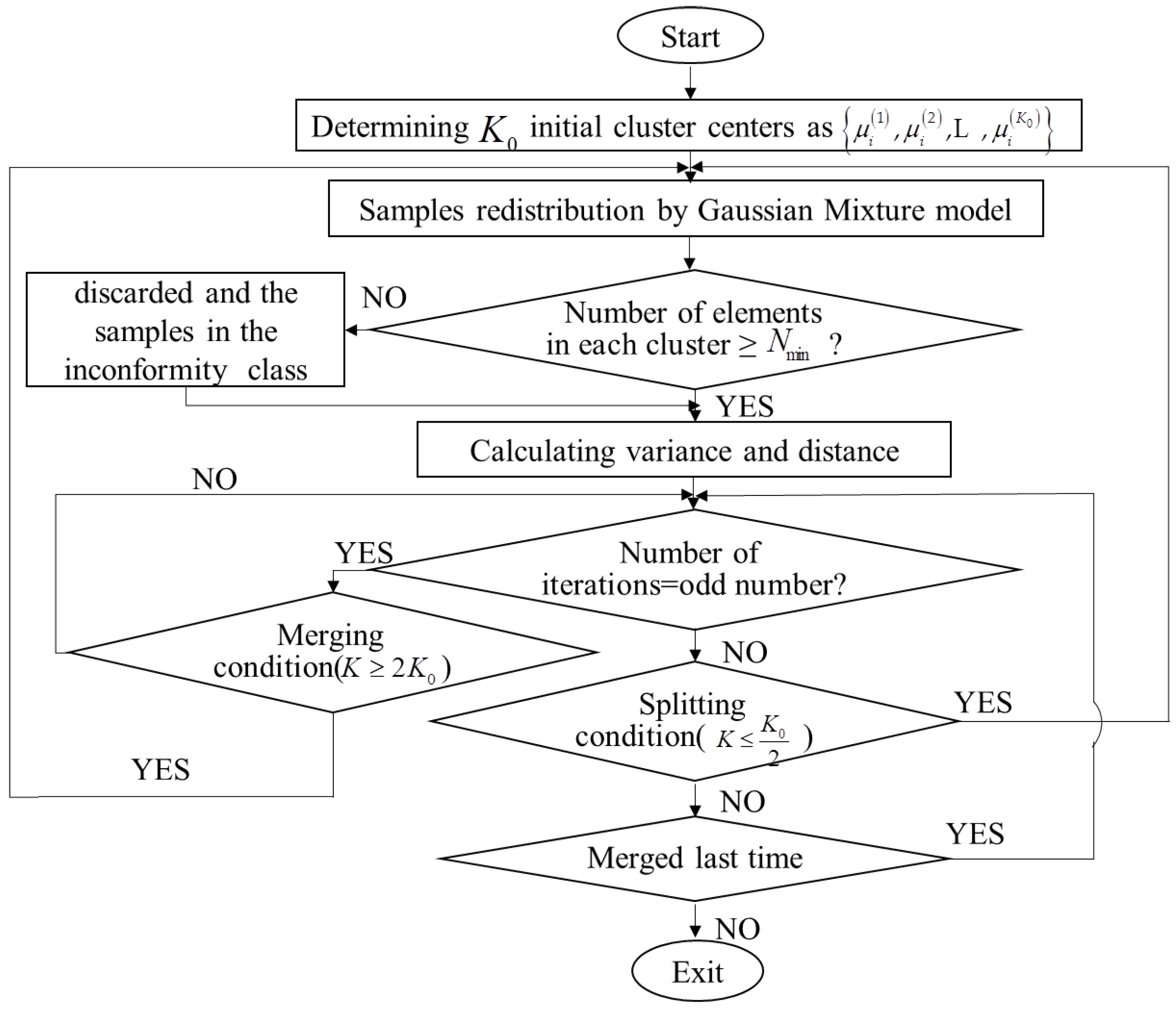
3.1. Clustering of the Monitoring Data Based on ISODATA-GMM
3.2. Random Coefficient Model
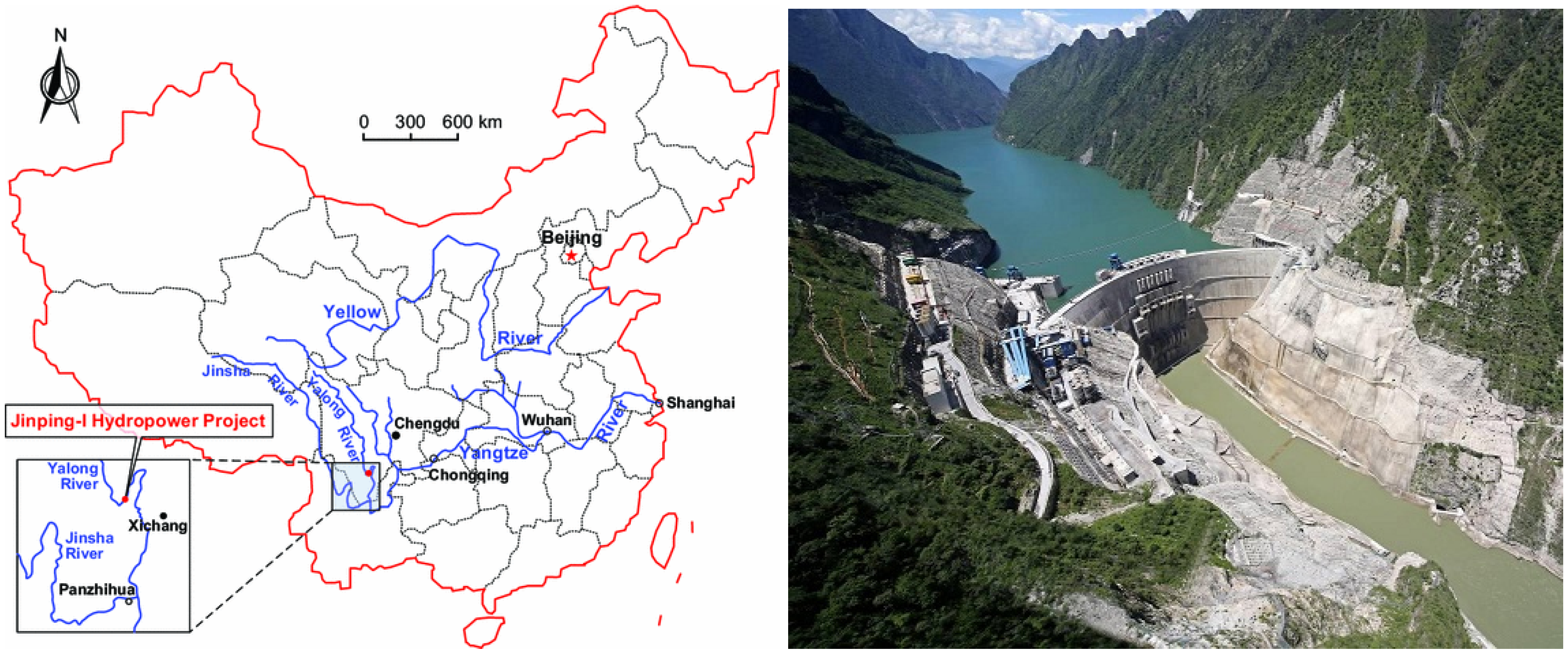
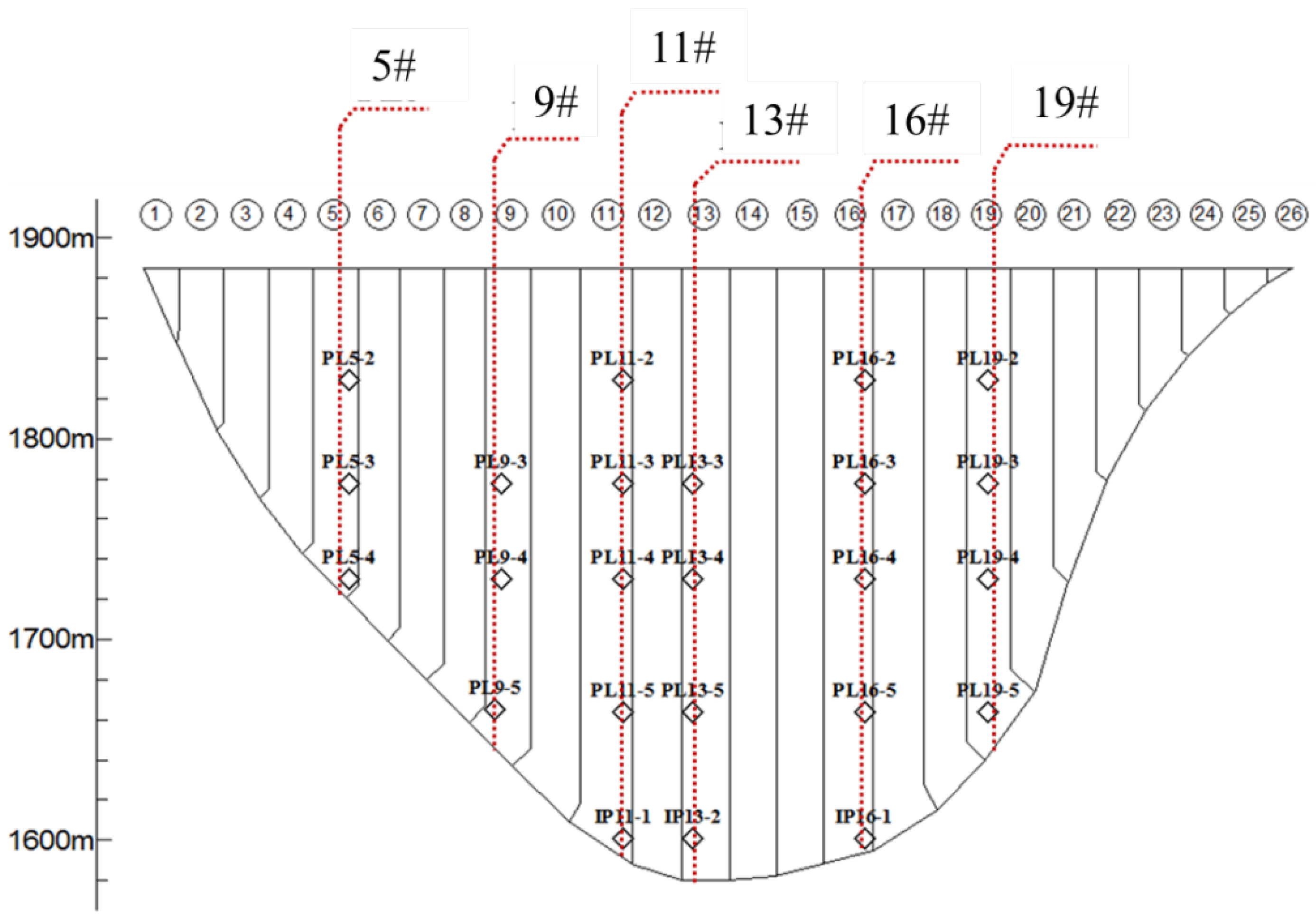
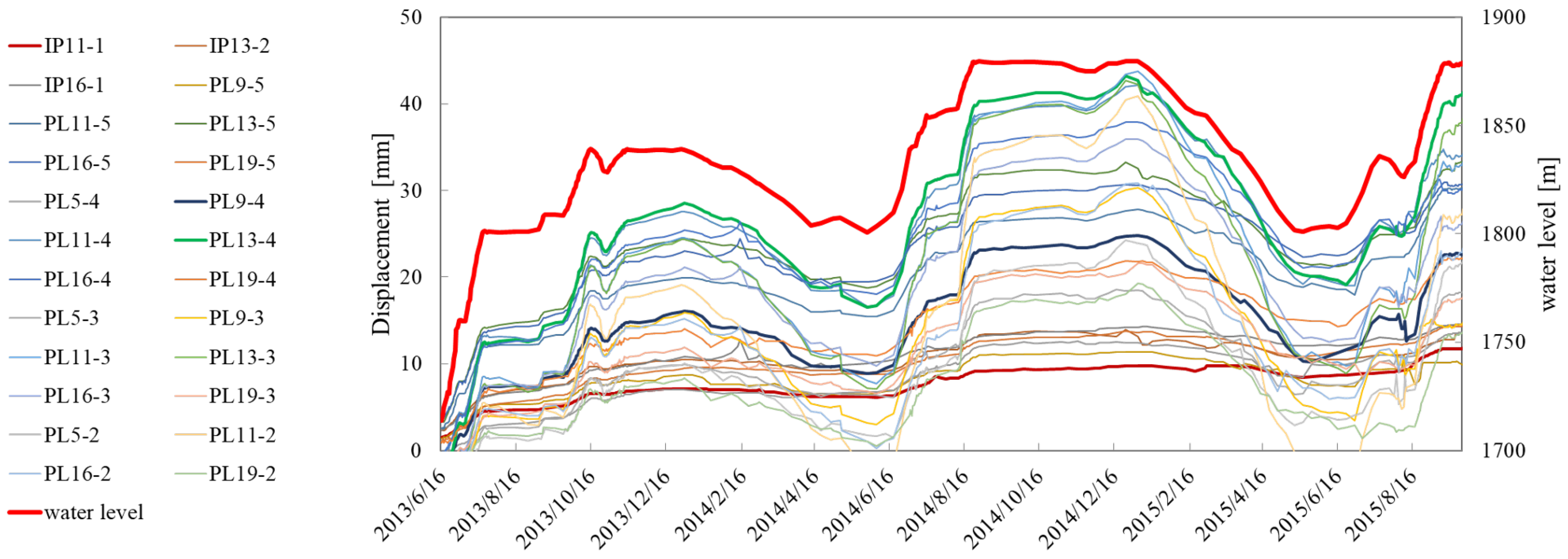
4. Data Sets
5. Results and Discussion
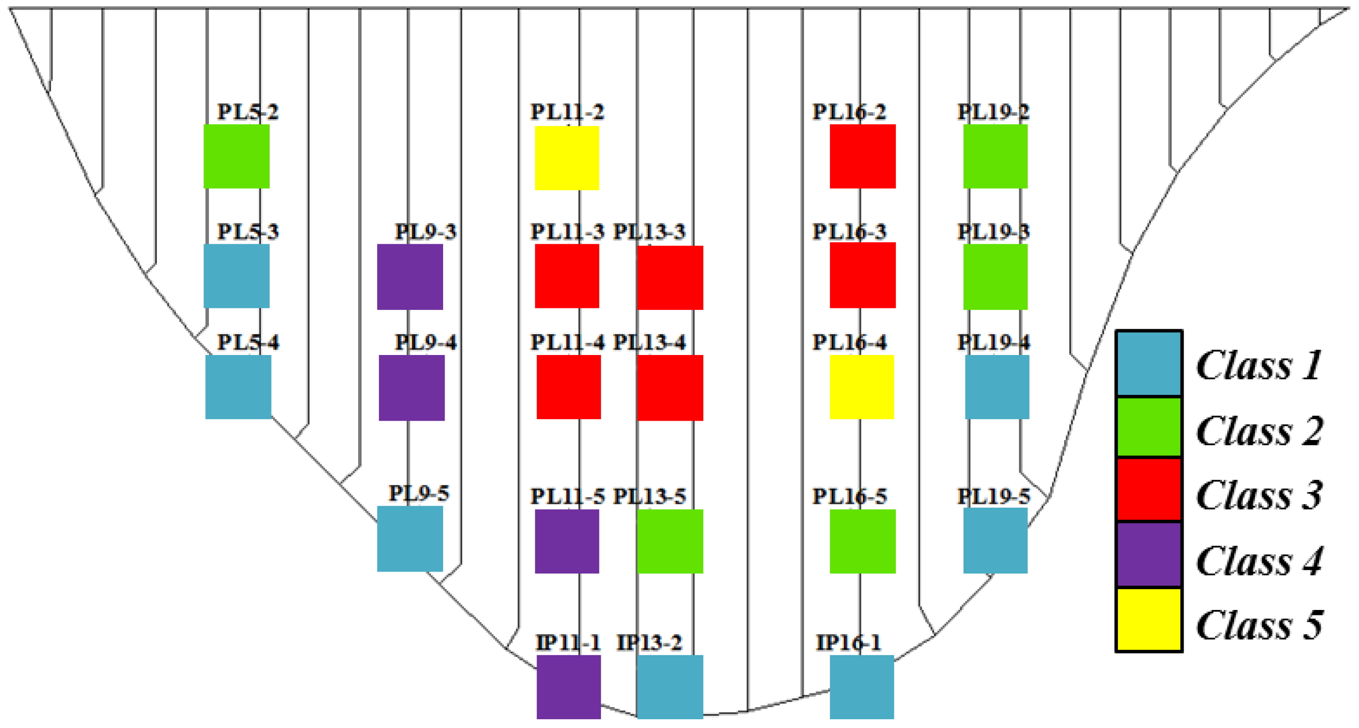
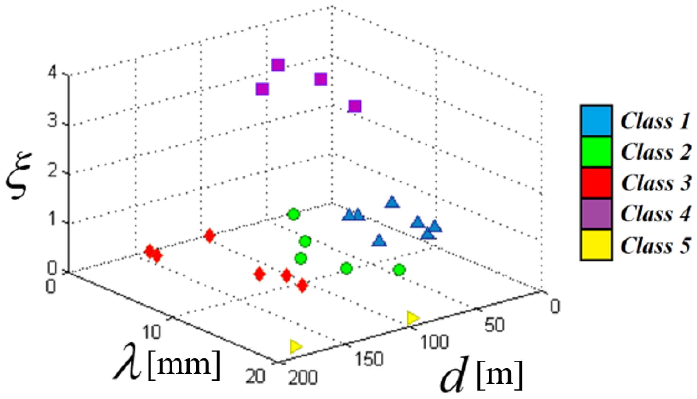
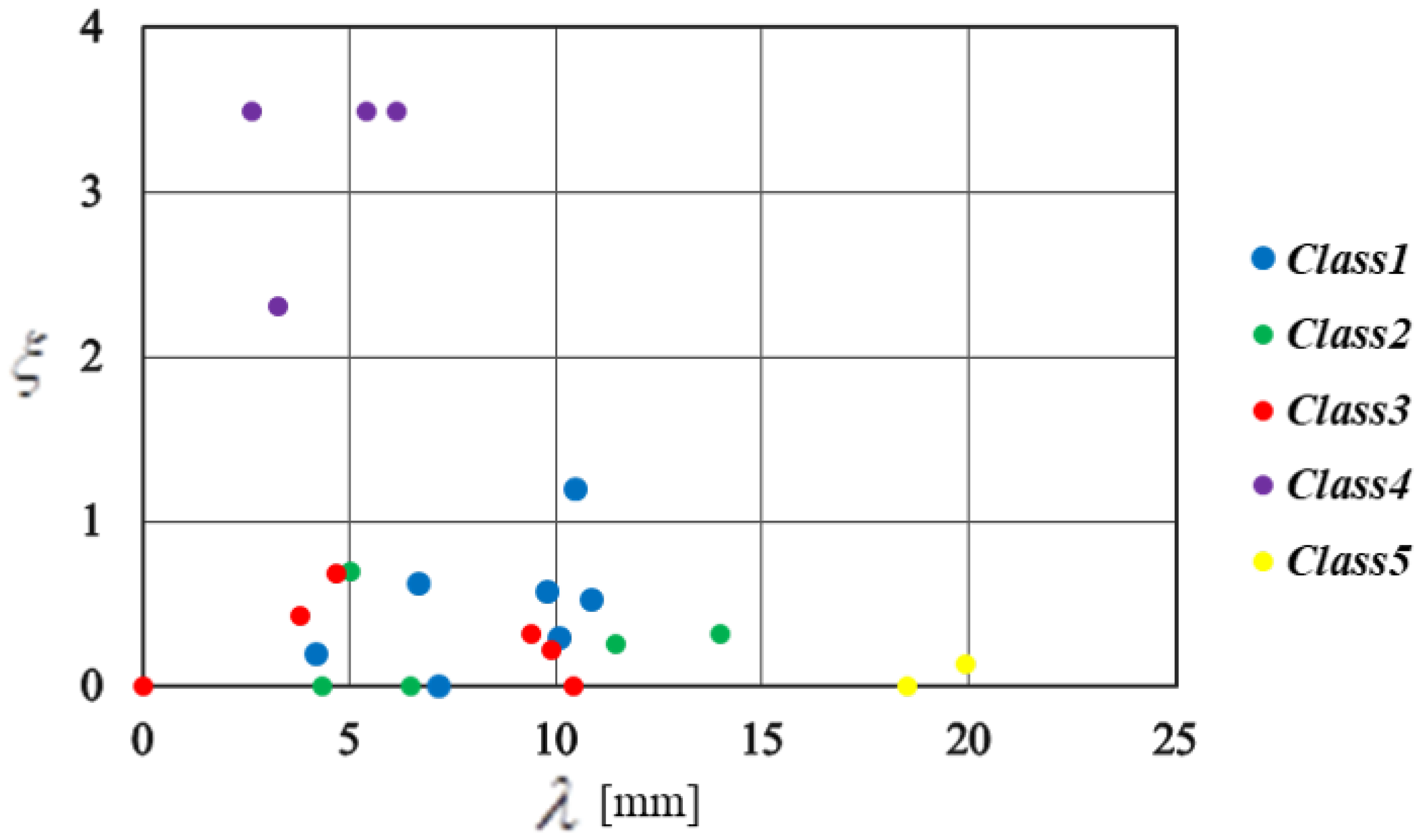
5.1. Clustering Results
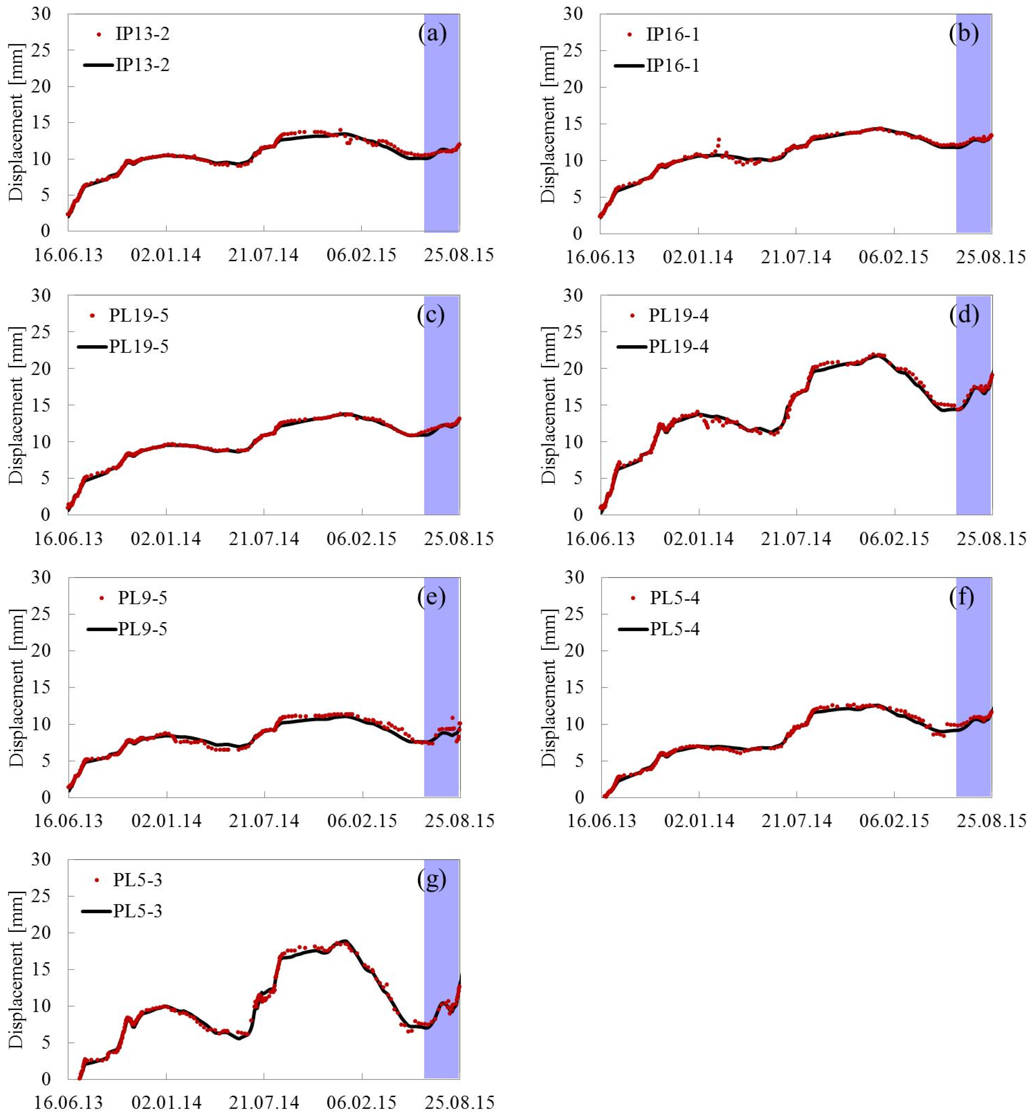
5.2. Predicting Results
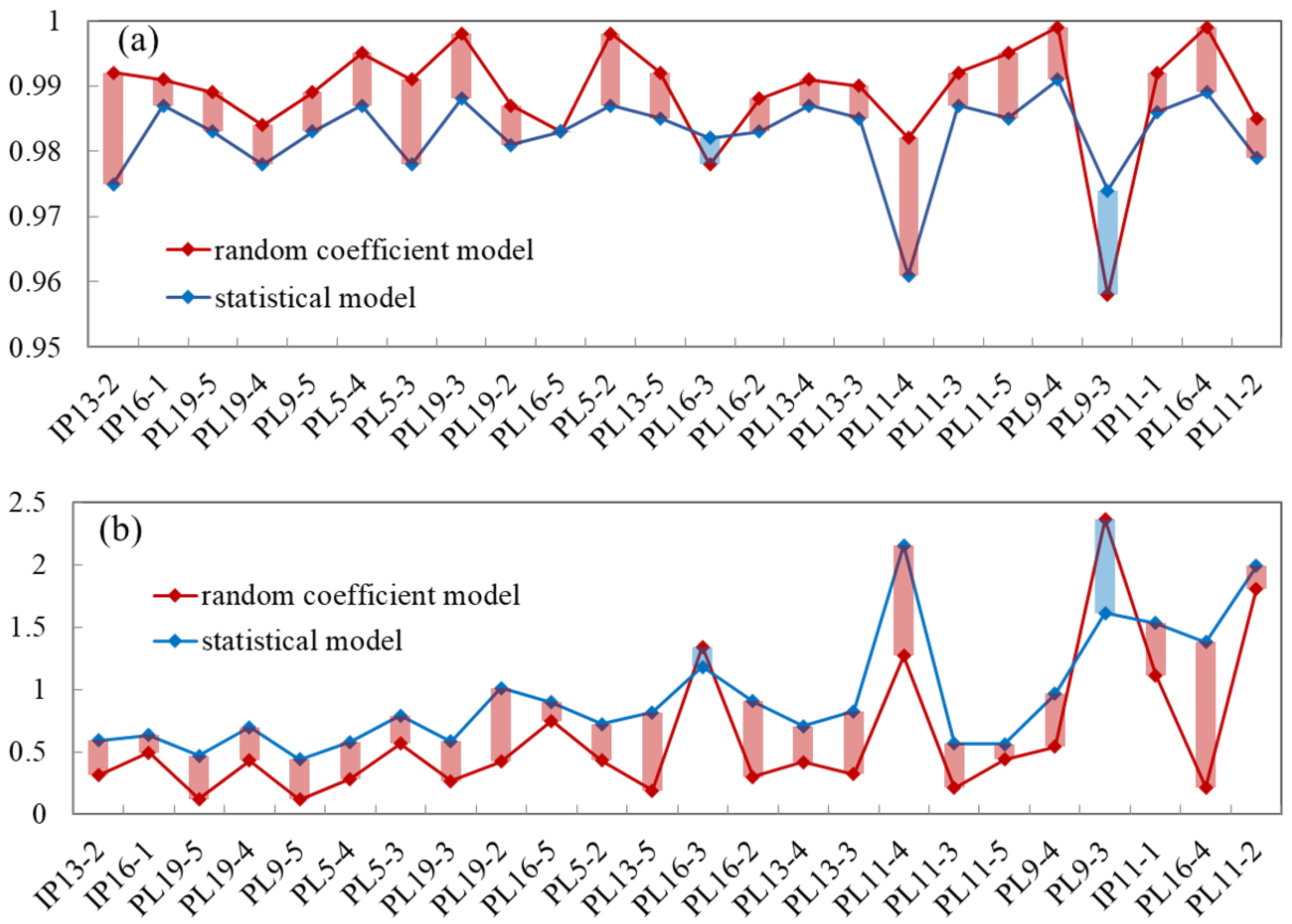
5.3. Comparison with the Statistical Model
5.4. Limitations
6. Conclusions
Author Contributions
Funding
Conflicts of Interest
Abbreviations
| GMM | Gaussian Mixture Model |
| ISODATA | Iterative Self-Organizing Data Analysis |
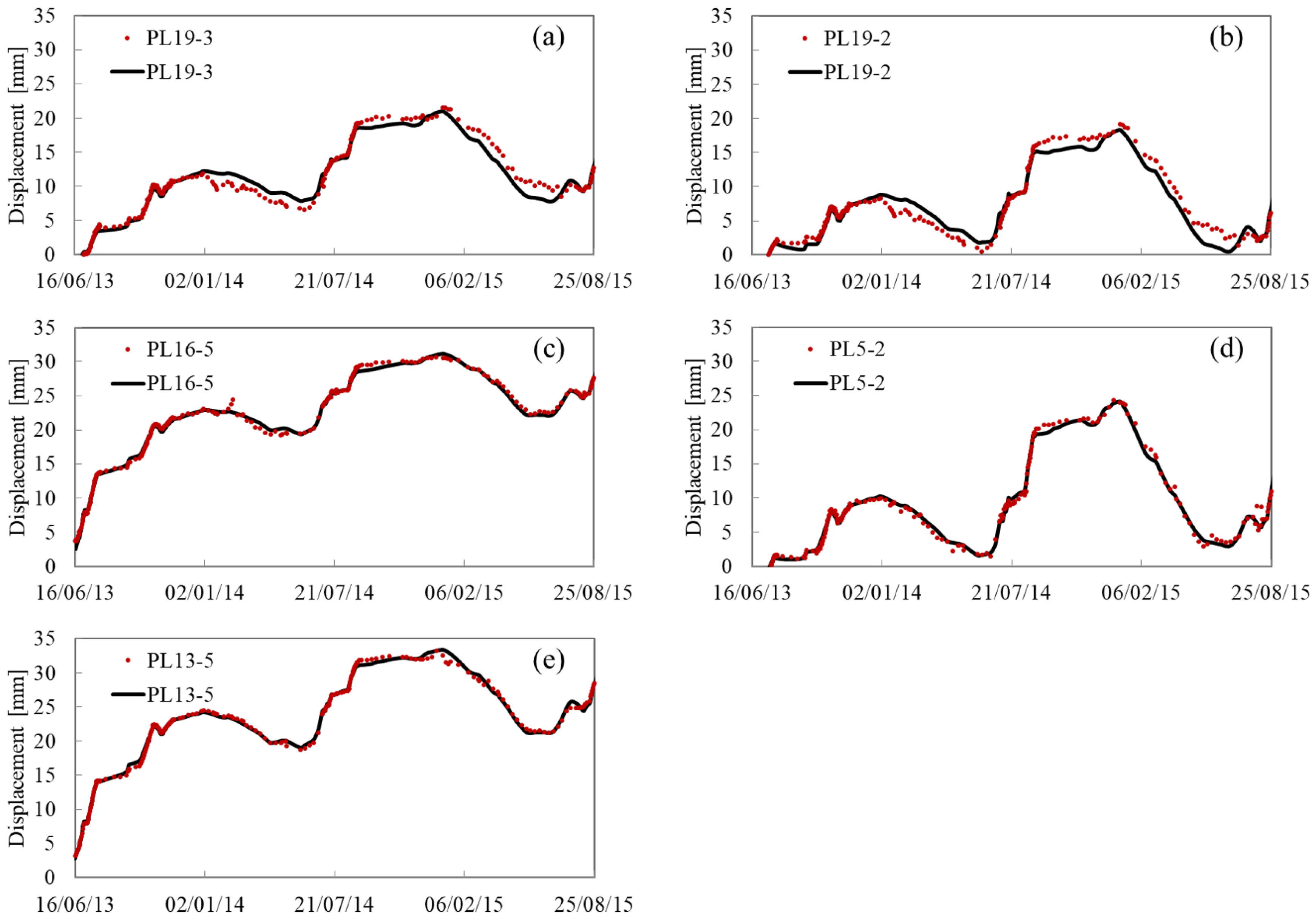
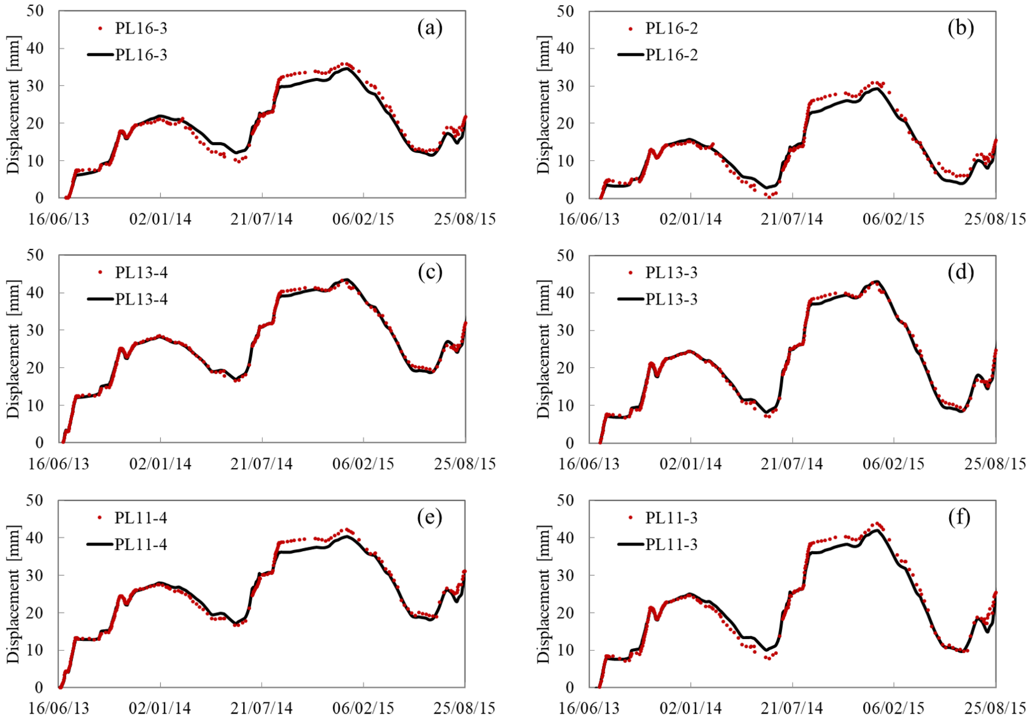
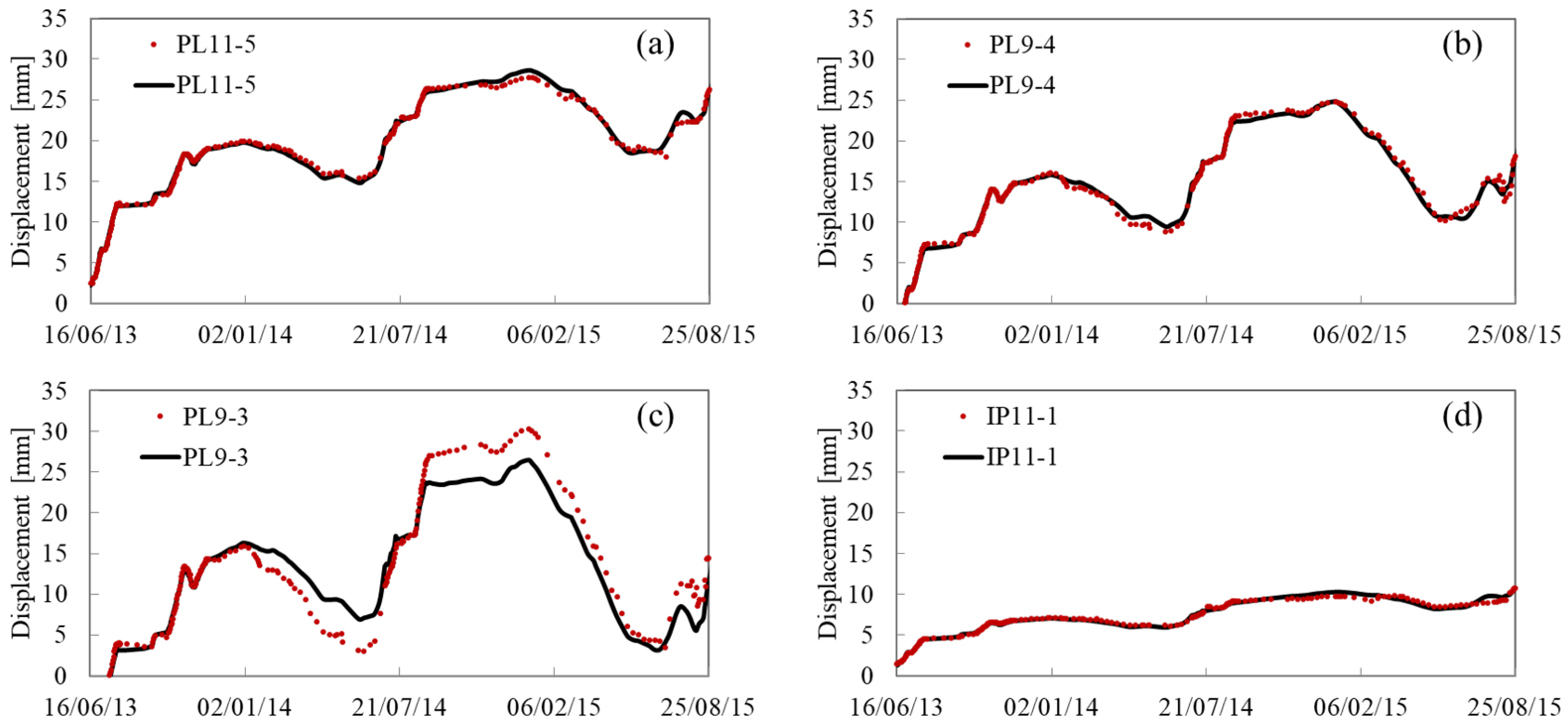
Appendix A. Fitting and Predicting Results

References
- Johansson, S. Seepage Monitoring in Embankment Dams. Ph.D. Thesis, Institutionen för anläggning och miljö, Uppsala, Sweden, 1997. [Google Scholar]
- Bonaldi, P.; Fanelli, M.; Giuseppetti, G. Displacement forecasting for concrete dams. Int. Water Power Dam Constr. 1977, 29, 42–45. [Google Scholar]
- Brownjohn, J.M. Structural health monitoring of civil infrastructure. Philos. Trans. R. Soc. A Math. Phys. Eng. Sci. 2006, 365, 589–622. [Google Scholar] [CrossRef] [PubMed]
- Léger, P.; Leclerc, M. Hydrostatic, temperature, time-displacement model for concrete dams. J. Eng. Mech. 2007, 133, 267–277. [Google Scholar] [CrossRef]
- De Sortis, A.; Paoliani, P. Statistical analysis and structural identification in concrete dam monitoring. Eng. Struct. 2007, 29, 110–120. [Google Scholar] [CrossRef]
- Mata, J.; Tavares de Castro, A.; Sá da Costa, J. Constructing statistical models for arch dam deformation. Struct. Control Health Monit. 2014, 21, 423–437. [Google Scholar] [CrossRef]
- Kao, C.Y.; Loh, C.H. Monitoring of long-term static deformation data of Fei-Tsui arch dam using artificial neural network-based approaches. Struct. Control Health Monit. 2013, 20, 282–303. [Google Scholar] [CrossRef]
- Wang, L.; Zhang, S.C.; Li, Y.H. Application of dynamic gray forecast model in dam deformation monitoring and forecast. J. Xi’an Univ. Sci. Technol. 2005, 3, 014. [Google Scholar]
- Xu, F.; Xu, W. Prediction of displacement time series based on support vector machines-Markov chain. Rock Soil Mech. 2010, 31, 944–948. [Google Scholar] [CrossRef]
- Zhang, H.; Xu, S. Multi-scale dam deformation prediction based on empirical mode decomposition and genetic algorithm for support vector machines (GA-SVM). Chin. J. Rock Mech. Eng. 2011, 30, 3681–3688. [Google Scholar]
- Chen, B.; Hu, T.; Huang, Z.; Fang, C. A spatio-temporal clustering and diagnosis method for concrete arch dams using deformation monitoring data. Struct. Health Monit. 2018. [Google Scholar] [CrossRef]
- Wooldridge, J.M. Fixed-effects and related estimators for correlated random-coefficient and treatment-effect panel data models. Rev. Econ. Stat. 2005, 87, 385–390. [Google Scholar] [CrossRef]
- Shao, C.; Gu, C.; Yang, M.; Xu, Y.; Su, H. A novel model of dam displacement based on panel data. Struct. Control Health Monit. 2018, 25, e2037. [Google Scholar] [CrossRef]
- Milligan, G.W.; Cooper, M.C. A study of the comparability of external criteria for hierarchical cluster analysis. Multivar. Behav. Res. 1986, 21, 441–458. [Google Scholar] [CrossRef] [PubMed]
- Huang, Z. Extensions to the k-means algorithm for clustering large data sets with categorical values. Data Min. Knowl. Discov. 1998, 2, 283–304. [Google Scholar] [CrossRef]
- Banfield, J.D.; Raftery, A.E. Model-based Gaussian and non-Gaussian clustering. Biometrics 1993, 49, 803–821. [Google Scholar] [CrossRef]
- Celeux, G.; Govaert, G. Gaussian parsimonious clustering models. Pattern Recognit. 1995, 28, 781–793. [Google Scholar] [CrossRef]
- Maugis, C.; Celeux, G.; Martin-Magniette, M.L. Variable selection for clustering with Gaussian mixture models. Biometrics 2009, 65, 701–709. [Google Scholar] [CrossRef] [PubMed]
- Wu, Z. Safety Monitoring Theory and Its Application of Hydraulic Structures; Higher Education: Beijing, China, 2003. [Google Scholar]
- Swamy, P.A. Efficient inference in a random coefficient regression model. Econom. J. Econom. Soc. 1970, 38, 311–323. [Google Scholar] [CrossRef]
- Wu, S.; Shen, M.; Wang, J. Jinping hydropower project: Main technical issues on engineering geology and rock mechanics. Bull. Eng. Geol. Environ. 2010, 69, 325–332. [Google Scholar]
- Xu, N.; Tang, C.; Li, L.; Zhou, Z.; Sha, C.; Liang, Z.; Yang, J. Microseismic monitoring and stability analysis of the left bank slope in Jinping first stage hydropower station in southwestern China. Int. J. Rock Mech. Min. Sci. 2011, 48, 950–963. [Google Scholar] [CrossRef]


| Measuring Point | d (m) | (mm) | (/) | Measuring Point | d (m) | (mm) | (/) |
|---|---|---|---|---|---|---|---|
| IP11-1 | 8 | 3.26 | 2.31 | PL11-5 | 58 | 6.16 | 3.49 |
| IP13-2 | 21 | 7.18 | 0 | PL13-3 | 163 | 3.8 | 0.43 |
| IP16-1 | 7 | 10.08 | 0.3 | PL13-4 | 130 | 9.39 | 0.32 |
| PL5-2 | 69 | 5.03 | 0.7 | PL13-5 | 80 | 11.46 | 0.26 |
| PL5-3 | 40 | 6.67 | 0.63 | PL16-2 | 131 | 4.71 | 0.68 |
| PL5-4 | 8 | 10.85 | 0.53 | PL16-3 | 113 | 9.88 | 0.22 |
| PL9-3 | 96 | 5.44 | 3.49 | PL16-4 | 98 | 19.93 | 0.13 |
| PL9-4 | 62 | 2.65 | 3.49 | PL16-5 | 60 | 13.96 | 0.32 |
| PL9-5 | 14 | 4.22 | 0.2 | PL19-2 | 76 | 6.51 | 0 |
| PL11-2 | 175 | 18.49 | 0 | PL19-3 | 55 | 4.36 | 0 |
| PL11-3 | 139 | 0 | 0 | PL19-4 | 38 | 10.47 | 1.2 |
| PL11-4 | 105 | 10.42 | 0 | PL19-5 | 13 | 9.79 | 0.57 |
| Measuring Point | R (-) | s (mm) | Measuring Point | R (-) | s (mm) |
|---|---|---|---|---|---|
| IP13-2 | 0.992 | 0.313 | PL16-3 | 0.978 | 1.344 |
| IP16-1 | 0.991 | 0.496 | PL16-2 | 0.988 | 0.302 |
| PL19-5 | 0.989 | 0.123 | PL13-4 | 0.991 | 0.221 |
| PL19-4 | 0.984 | 0.432 | PL13-3 | 0.99 | 0.321 |
| PL9-5 | 0.989 | 0.121 | PL11-4 | 0.982 | 1.27 |
| PL5-4 | 0.995 | 0.283 | PL11-3 | 0.992 | 0.211 |
| PL5-3 | 0.991 | 0.568 | PL11-5 | 0.995 | 0.142 |
| PL19-3 | 0.998 | 0.268 | PL9-4 | 0.999 | 0.542 |
| PL19-2 | 0.987 | 0.423 | PL9-3 | 0.958 | 0.363 |
| PL16-5 | 0.983 | 0.752 | IP11-1 | 0.992 | 1.116 |
| PL5-2 | 0.998 | 0.433 | PL16-4 | 0.999 | 0.215 |
| PL13-5 | 0.992 | 0.193 | PL11-2 | 0.985 | 1.809 |
© 2019 by the authors. Licensee MDPI, Basel, Switzerland. This article is an open access article distributed under the terms and conditions of the Creative Commons Attribution (CC BY) license (http://creativecommons.org/licenses/by/4.0/).
Share and Cite
Hu, Y.; Shao, C.; Gu, C.; Meng, Z. Concrete Dam Displacement Prediction Based on an ISODATA-GMM Clustering and Random Coefficient Model. Water 2019, 11, 714. https://doi.org/10.3390/w11040714
Hu Y, Shao C, Gu C, Meng Z. Concrete Dam Displacement Prediction Based on an ISODATA-GMM Clustering and Random Coefficient Model. Water. 2019; 11(4):714. https://doi.org/10.3390/w11040714
Chicago/Turabian StyleHu, Yating, Chenfei Shao, Chongshi Gu, and Zhenzhu Meng. 2019. "Concrete Dam Displacement Prediction Based on an ISODATA-GMM Clustering and Random Coefficient Model" Water 11, no. 4: 714. https://doi.org/10.3390/w11040714
APA StyleHu, Y., Shao, C., Gu, C., & Meng, Z. (2019). Concrete Dam Displacement Prediction Based on an ISODATA-GMM Clustering and Random Coefficient Model. Water, 11(4), 714. https://doi.org/10.3390/w11040714