Designing an Optimized Water Quality Monitoring Network with Reserved Monitoring Locations


Abstract
:1. Introduction
2. Related Technologies
2.1. SWMM
2.2. Pareto Frontier
2.3. MOPSO Algorithm
2.4. Closeness Centrality
3. Methodology
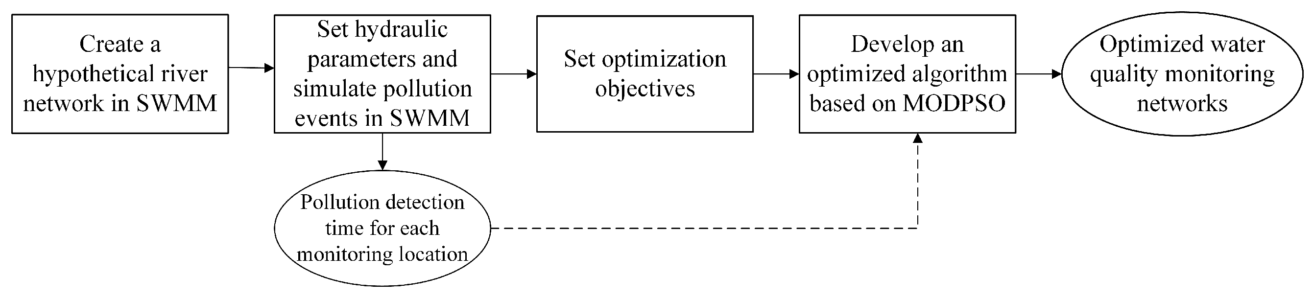
3.1. Main Process of Our Algorithm
3.2. Hydrodynamic Simulations
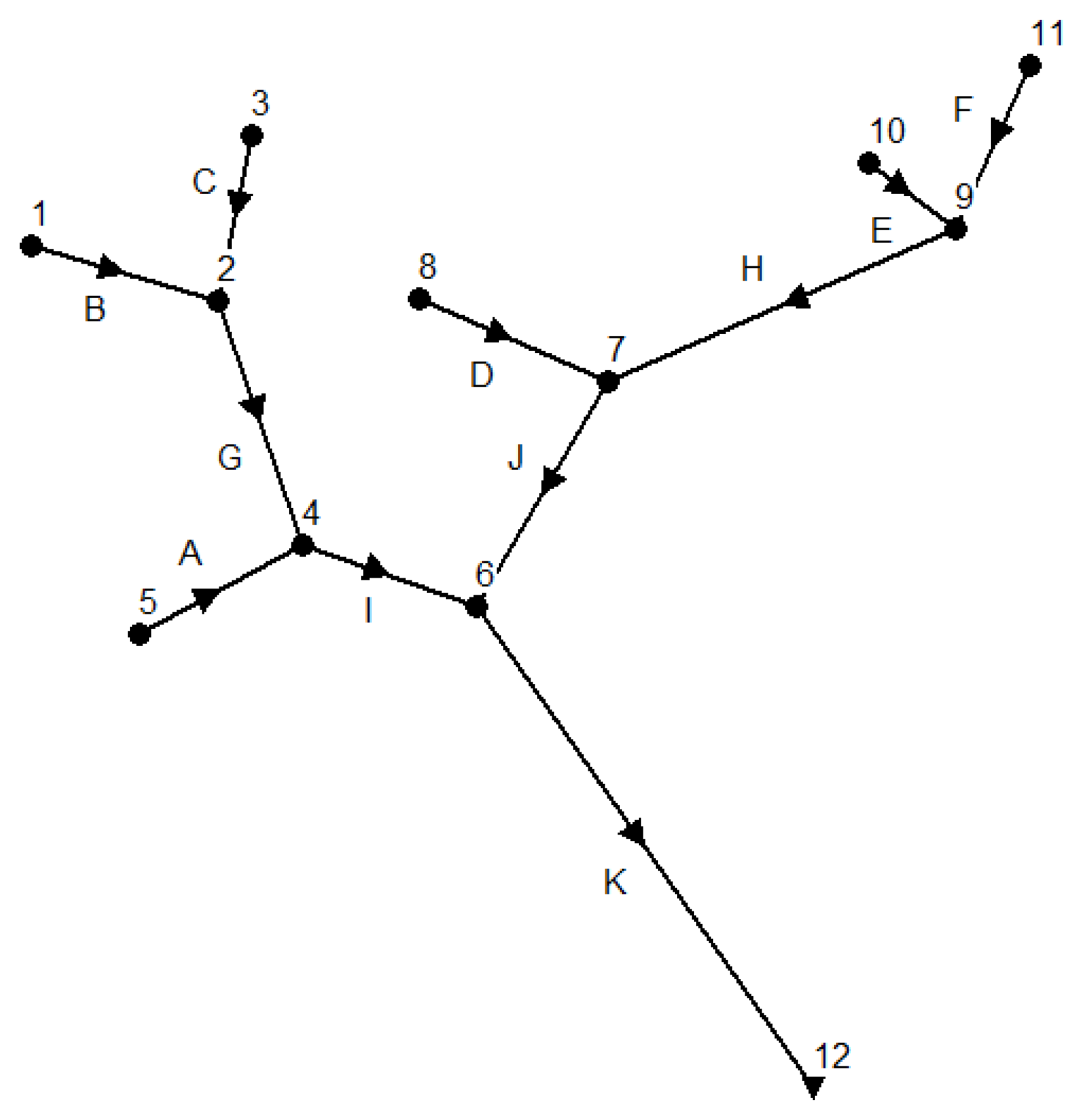
3.2.1. Hypothetical River Network
3.2.2. SWMM Simulations
3.3. Optimization Objectives
3.3.1. Minimum Pollution Detection Time
3.3.2. Maximum Pollution Detection Probability
3.3.3. Maximum Closeness Centrality of Monitoring Locations
3.3.4. Reservation of Monitoring Locations
3.4. Improved Algorithm of MODPSO
3.4.1. Particle Design and Swarm Initialization
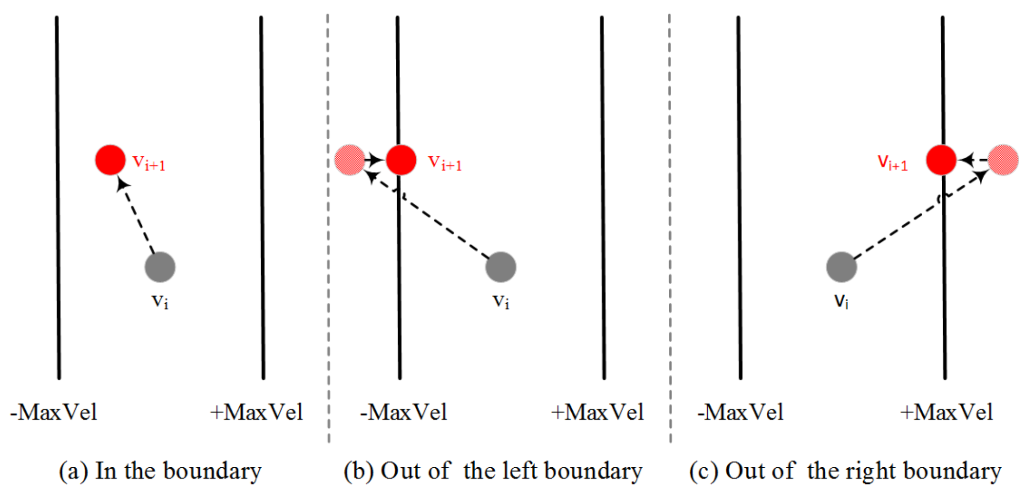
3.4.2. Velocity and Position Updating
3.4.3. Reserved Monitoring Locations
3.4.4. Dominance Evaluation
4. Simulations and Analysis
4.1. Simulation with Two Objectives of Maximum Pollution Detection Probability and Minimum Pollution Detection Time
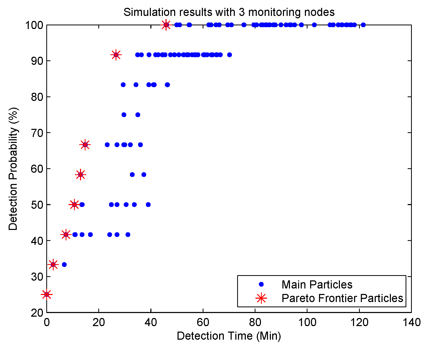
4.2. Simulation with Three Objectives of Maximum Pollution Detection Probability, Minimum Pollution Detection Time and Maximum Centrality
4.3. Simulation with All Four Optimization Objectives
4.4. Computational Time Analysis with More Potential Monitoring Locations
5. Conclusions and Future Work
Author Contributions
Funding
Conflicts of Interest
Appendix A
| Algorithm A1 Pseudocode of MOPSO |
| procedure MOPSO Step 1. Initialization (1) Initialize all parameters (e.g., size of population and repository, maximum number of iterations, lower and upper bounds of search space) (2) For each do (a) Initialize the particle’s position randomly (b) Initialize with its initial position (c) Initialize particle’s velocity = 0 (3) Calculate non-domination particles using cost function (4) Initialize with a particle selected from non-domination particles using a roulette wheel selection. Step 2. Repeat until the termination criteria is satisfied or to the maximum number of iterations (5) For each do (a) Calculate particle’s new velocity using Equation (7) (b) Calculate particle’s new position using Equation (8) (c) Update particle’s (d) Calculate non-domination particles using cost function (e) = a particle selected from non-domination particles using a roulette wheel selection. Step 3. Output non-domination particles. end procedure |
| Algorithm A2 Pseudocode of MODPSO initialization |
| procedureInitialization(k)
fori = 1 to k do for j = 1 to n do end for end for end procedure |
| Algorithm A3 Pseudocode of velocity and position updating |
| procedureVel_Pos_Updating(k)
fori = 1 to k do for j = 1 to n do if then end if end for end for end procedure |
| Algorithm A4 Pseudocode of MODPSO initialization with reserved locations |
| procedureInitWithReservedLocations(k) fori = 1 to k do for t = 1 to R do end for for j = to n do end for end for end procedure |
| Algorithm A5 Pseudocode of velocity and position updating with reserved locations |
| procedureNew_Vel_Pos_Updating(k) fori = 1 to k do for to n do if then end if end for end for end procedure |
| Algorithm A6 Pseudocode of cost function |
| procedureCost(p) Array for each in do for each l in do end for if then end if end for for each l in do end for return end procedure |
References
- Skoczko, I.; Struk-Sokolowska, J.; Ofman, P. Modelling Changes in the Parameters of Treated Sewage Using Artificial Neural Networks. Rocz. Ochr. Srodowiska 2017, 19, 633–650. [Google Scholar]
- Skoczko, I.; Ofman, P.; Szatylowicz, E. Using Artificial Neural Networks for Modeling Wastewater Treatment in Small Wastewater Treatment Plant. Rocz. Ochr. Srodowiska 2016, 18, 493–506. [Google Scholar]
- Yang, Y. How to Look at the GDP Receiving Much Attention. Revolution 2015, 12, 26–32. [Google Scholar]
- Behmel, S.; Damour, M.; Ludwig, R.; Rodriguez, M.J. Water quality monitoring strategies—A review and future perspectives. Sci. Total Environ. 2016, 571, 1312–1329. [Google Scholar] [CrossRef] [PubMed]
- Park, S.Y.; Choi, J.H.; Wang, S.; Park, S.S. Design of a water quality monitoring network in a large river system using the genetic algorithm. Ecol. Model. 2006, 199, 289–297. [Google Scholar] [CrossRef]
- Chilundo, M.; Kelderman, P. Design of a water quality monitoring network for the Limpopo River Basin in Mozambique. Phys. Chem. Earth 2008, 33, 655–665. [Google Scholar] [CrossRef]
- Chang, C.L.; Lin, Y.T. A water quality monitoring network design using fuzzy theory and multiple criteria analysis. Environ. Monit. Assess. 2014, 186, 6459–6469. [Google Scholar] [CrossRef]
- Storey, M.V.; Van der Gaag, B.; Burns, B.P. Advances in on-line drinking water quality monitoring and early warning systems. Water Res. 2011, 45, 741–747. [Google Scholar] [CrossRef]
- Lambrou, T.P.; Anastasiou, C.C.; Panayiotou, C.G.; Polycarpou, M.M. A low-cost sensor network for real-time monitoring and contamination detection in drinking water distribution systems. IEEE Sens. J. 2014, 14, 2765–2772. [Google Scholar] [CrossRef]
- Borgatti, S.P.; Everett, M.G. A graph-theoretic perspective on centrality. Soc. Netw. 2006, 28, 466–484. [Google Scholar] [CrossRef]
- Ouyang, H.T.; Yu, H.; Lu, C.H.; Luo, Y.H. Design optimization of river sampling network using genetic algorithms. J. Water Resour. Plan. Manag. 2008, 134, 83–87. [Google Scholar] [CrossRef]
- Telci, I.T.; Nam, K.; Guan, J.; Aral, M.M. Real time optimal monitoring network design in river networks. In World Environmental and Water Resources Congress 2008: Ahupua’A 2008; ASCE: Reston, VA, USA, 2008; pp. 1–10. [Google Scholar]
- Telci, I.T.; Nam, K.; Guan, J.; Aral, M.M. Optimal water quality monitoring network design for river systems. J. Environ. Manag. 2009, 90, 2987–2998. [Google Scholar] [CrossRef] [PubMed]
- Park, C. Discrete Optimization via Simulation with Stochastic Constraints. Ph.D. Thesis, Georgia Institute of Technology, Atlanta, GA, USA, 2013. [Google Scholar]
- Rossman, L.A. Storm Water Management Model User’s Manual, Version 5.0; National Risk Management Research Laboratory, Office of Research and Development, US Environmental Protection Agency: Cincinnati, OH, USA, 2010; p. 276.
- Xing, W.; Li, P.; Cao, S.B.; Gan, L.L.; Liu, F.L.; Zuo, J.E. Layout effects and optimization of runoff storage and filtration facilities based on SWMM simulation in a demonstration area. Water Sci. Eng. 2016, 9, 115–124. [Google Scholar] [CrossRef]
- Mukhopadhyay, A.; Maulik, U.; Bandyopadhyay, S.; Coello, C.A.C. A survey of multiobjective evolutionary algorithms for data mining: Part I. IEEE Trans. Evol. Comput. 2014, 18, 4–19. [Google Scholar] [CrossRef]
- Kalyanmoy, D. Multi Objective Optimization Using Evolutionary Algorithms; John Wiley and Sons: Hoboken, NJ, USA, 2001. [Google Scholar]
- Eberhart, R.C.; Shi, Y. Comparison between genetic algorithms and particle swarm optimization. In International Conference on Evolutionary Programming; Springer: Berlin/Heidelberg, Germany, 1998; pp. 611–616. [Google Scholar]
- Reyes-Sierra, M.; Coello, C.C. Multi-objective particle swarm optimizers: A survey of the state-of-the-art. Int. J. Comput. Intell. Res. 2006, 2, 287–308. [Google Scholar]
- Coello, C.C.; Lechuga, M.S. MOPSO: A proposal for multiple objective particle swarm optimization. In Proceedings of the 2002 Congress on Evolutionary Computation, Honolulu, HI, USA, 12–17 May 2002; Volume 2, pp. 1051–1056. [Google Scholar]
- Coello, C.A.C.; Pulido, G.T.; Lechuga, M.S. Handling multiple objectives with particle swarm optimization. IEEE Trans. Evol. Comput. 2004, 8, 256–279. [Google Scholar] [CrossRef]
- Ezzeldin, R.; Djebedjian, B.; Saafan, T. Integer discrete particle swarm optimization of water distribution networks. J. Pipeline Syst. Eng. Pract. 2013, 5, 04013013. [Google Scholar] [CrossRef]
- Kennedy, J.; Eberhart, R.C. A discrete binary version of the particle swarm algorithm. In Proceedings of the 1997 IEEE International Conference on Systems, Man, and Cybernetics. Computational Cybernetics and Simulation, Orlando, FL, USA, 12–15 October 1997; Volume 5, pp. 4104–4108. [Google Scholar]
- Chen, W.N.; Zhang, J.; Chung, H.S.; Zhong, W.L.; Wu, W.G.; Shi, Y.H. A novel set-based particle swarm optimization method for discrete optimization problems. IEEE Trans. Evol. Comput. 2010, 14, 278–300. [Google Scholar] [CrossRef]
- Aminbakhsh, S.; Sonmez, R. Discrete particle swarm optimization method for the large-scale discrete time–cost trade-off problem. Expert Syst. Appl. 2016, 51, 177–185. [Google Scholar] [CrossRef]
- Venkatesan, S.P.; Kumanan, S. A multi-objective discrete particle swarm optimisation algorithm for supply chain network design. Int. J. Logist. Syst. Manag. 2012, 11, 375–406. [Google Scholar] [CrossRef]
- Cui, Z.; Koren, V.; Cajina, N.; Voellmy, A.; Moreda, F. Hydroinformatics advances for operational river forecasting: Using graphs for drainage network descriptions. J. Hydroinformat. 2011, 13, 181–197. [Google Scholar] [CrossRef]
- Phillips, J.D.; Schwanghart, W.; Heckmann, T. Graph theory in the geosciences. Earth-Sci. Rev. 2015, 143, 147–160. [Google Scholar] [CrossRef]
- Heckmann, T.; Schwanghart, W.; Phillips, J.D. Graph theory—Recent developments of its application in geomorphology. Geomorphology 2015, 243, 130–146. [Google Scholar] [CrossRef]
- Freeman, L.C. Centrality in social networks conceptual clarification. Soc. Netw. 1978, 1, 215–239. [Google Scholar] [CrossRef]
- Nathan, E.; Sanders, G.; Bader, D.A. Numerically approximating centrality for graph ranking guarantees. J. Comput. Sci. 2018, 26, 205–216. [Google Scholar] [CrossRef]
- Strobl, R.; Robillard, P.D. Network design for water quality monitoring of surface freshwaters: A review. J. Environ. Manag. 2008, 87, 639–648. [Google Scholar] [CrossRef] [PubMed]
- Loaiciga, H.A. An optimization approach for groundwater quality monitoring network design. Water Resour. Res. 1989, 25, 1771–1782. [Google Scholar] [CrossRef]


| Catchment | Width | Channel | Manning’s | Length | Flow Rate |
|---|---|---|---|---|---|
| (m) | Slope | Coefficient | (m) | (L/s) | |
| A | 3.048 | 0.0001 | 0.02 | 609.6 | 283.168 |
| B | 3.048 | 0.0001 | 0.02 | 609.6 | 283.168 |
| C | 3.048 | 0.0001 | 0.02 | 609.6 | 283.168 |
| D | 3.048 | 0.0001 | 0.02 | 609.6 | 283.168 |
| E | 3.048 | 0.0001 | 0.02 | 304.8 | 283.168 |
| F | 3.048 | 0.0001 | 0.02 | 609.6 | 283.168 |
| G | 3.048 | 0.0001 | 0.02 | 914.4 | 566.336 |
| H | 3.048 | 0.0001 | 0.02 | 1219.2 | 566.336 |
| I | 3.048 | 0.0001 | 0.02 | 609.6 | 849.504 |
| J | 3.048 | 0.0001 | 0.02 | 914.4 | 849.504 |
| K | 3.048 | 0.0001 | 0.02 | 1524 | 1699.008 |
| Pollution Locations | Pollution Detection Time (min) for Potential Monitoring Locations | |||||||||||
|---|---|---|---|---|---|---|---|---|---|---|---|---|
| 1 | 2 | 3 | 4 | 5 | 6 | 7 | 8 | 9 | 10 | 11 | 12 | |
| 1 | 0 | 27 | _ | 81 | _ | 118 | _ | _ | _ | _ | _ | 198 |
| 2 | _ | 0 | _ | 40 | _ | 75 | _ | _ | _ | _ | _ | 152 |
| 3 | _ | 27 | 0 | 81 | _ | 118 | _ | _ | _ | _ | _ | 198 |
| 4 | _ | _ | _ | 0 | _ | 23 | _ | _ | _ | _ | _ | 96 |
| 5 | _ | _ | _ | 28 | 0 | 62 | _ | _ | _ | _ | _ | 139 |
| 6 | _ | _ | _ | _ | _ | 0 | _ | _ | _ | _ | _ | 62 |
| 7 | _ | _ | _ | _ | _ | 38 | 0 | _ | _ | _ | _ | 113 |
| 8 | _ | _ | _ | _ | _ | 79 | 27 | 0 | _ | _ | _ | 157 |
| 9 | _ | _ | _ | _ | _ | 111 | 57 | _ | 0 | _ | _ | 190 |
| 10 | _ | _ | _ | _ | _ | 133 | 78 | _ | 10 | 0 | _ | 213 |
| 11 | _ | _ | _ | _ | _ | 156 | 99 | _ | 27 | _ | 0 | 236 |
| 12 | _ | _ | _ | _ | _ | _ | _ | _ | _ | _ | _ | 0 |
| Pollution Locations | Pollution Detection Time (min) for Potential Monitoring Locations | |||||||||||
|---|---|---|---|---|---|---|---|---|---|---|---|---|
| 1 | 2 | 3 | 4 | 5 | 6 | 7 | 8 | 9 | 10 | 11 | 12 | |
| 1 | 0 | 44 | _ | 112 | _ | 165 | _ | _ | _ | _ | _ | 253 |
| 2 | _ | 0 | _ | 61 | _ | 110 | _ | _ | _ | _ | _ | 199 |
| 3 | _ | 44 | 0 | 112 | _ | 165 | _ | _ | _ | _ | _ | 253 |
| 4 | _ | _ | _ | 0 | _ | 42 | _ | _ | _ | _ | _ | 131 |
| 5 | _ | _ | _ | 47 | 0 | 97 | _ | _ | _ | _ | _ | 186 |
| 6 | _ | _ | _ | _ | _ | 0 | _ | _ | _ | _ | _ | 90 |
| 7 | _ | _ | _ | _ | _ | 62 | 0 | _ | _ | _ | _ | 152 |
| 8 | _ | _ | _ | _ | _ | 116 | 47 | 0 | _ | _ | _ | 205 |
| 9 | _ | _ | _ | _ | _ | 153 | 82 | _ | 0 | _ | _ | 242 |
| 10 | _ | _ | _ | _ | _ | 181 | 108 | _ | 20 | 0 | _ | 269 |
| 11 | _ | _ | _ | _ | _ | 208 | 134 | _ | 44 | _ | 0 | 297 |
| 12 | _ | _ | _ | _ | _ | _ | _ | _ | _ | _ | _ | 0 |
| Pollution Locations | Pollution Detection Time (min) for Potential Monitoring Locations | |||||||||||
|---|---|---|---|---|---|---|---|---|---|---|---|---|
| 1 | 2 | 3 | 4 | 5 | 6 | 7 | 8 | 9 | 10 | 11 | 12 | |
| 1 | 0 | 50 | _ | 124 | _ | _ | _ | _ | _ | _ | _ | _ |
| 2 | _ | 0 | _ | 69 | _ | _ | _ | _ | _ | _ | _ | _ |
| 3 | _ | 50 | 0 | 124 | _ | _ | _ | _ | _ | _ | _ | _ |
| 4 | _ | _ | _ | 0 | _ | _ | _ | _ | _ | _ | _ | _ |
| 5 | _ | _ | _ | 55 | 0 | _ | _ | _ | _ | _ | _ | _ |
| 6 | _ | _ | _ | _ | _ | _ | _ | _ | _ | _ | _ | _ |
| 7 | _ | _ | _ | _ | _ | _ | 0 | _ | _ | _ | _ | _ |
| 8 | _ | _ | _ | _ | _ | _ | 55 | 0 | _ | _ | _ | _ |
| 9 | _ | _ | _ | _ | _ | _ | 92 | _ | 0 | _ | _ | _ |
| 10 | _ | _ | _ | _ | _ | _ | 119 | _ | 24 | 0 | _ | _ |
| 11 | _ | _ | _ | _ | _ | _ | 146 | _ | 50 | _ | 0 | _ |
| 12 | _ | _ | _ | _ | _ | _ | _ | _ | _ | _ | _ | _ |
| Monitoring Locations | Detection Time (min) | Detection Probability |
|---|---|---|
| 6, 9, 12 | 45.8 | 100% |
| 2, 6, 9 | 26.6 | 91.7% |
| 2, 7, 9 | 14.8 | 66.7% |
| 2, 5, 9 | 13 | 58.3% |
| 2, 8, 9 | 13 | 58.3% |
| 1, 7, 9 | 10.7 | 50% |
| 3, 7, 9 | 10.7 | 50% |
| 5, 7, 9 | 10.7 | 50% |
| 1, 5, 9 | 7.4 | 41.7% |
| 1, 8, 9 | 7.4 | 41.7% |
| 3, 5, 9 | 7.4 | 41.7% |
| 3, 8, 9 | 7.4 | 41.7% |
| 5, 8, 9 | 7.4 | 41.7% |
| 7, 8, 9 | 7.4 | 41.7% |
| 7, 9, 11 | 7.4 | 41.7% |
| 1, 9, 11 | 2.5 | 33.3% |
| 5, 9, 11 | 2.5 | 33.3% |
| 8, 9, 11 | 2.5 | 33.3% |
| 1, 5, 10 | 0 | 25% |
| 1, 5, 11 | 0 | 25% |
| 3, 5, 8 | 0 | 25% |
| 3, 5, 10 | 0 | 25% |
| 3, 8, 10 | 0 | 25% |
| 5, 8, 10 | 0 | 25% |
| 5, 8, 11 | 0 | 25% |
| 5, 10, 11 | 0 | 25% |
| 8, 10, 11 | 0 | 25% |
| Monitoring Locations | Detection Time (min) | Detection Probability |
|---|---|---|
| 6, 9, 12 | 68.4 | 100% |
| 2, 6, 9 | 42.6 | 91.7% |
| 2, 7, 9 | 24.9 | 66.7% |
| 2, 5, 9 | 21.7 | 58.3% |
| 2, 8, 9 | 21.7 | 58.3% |
| 2, 3, 9 | 18 | 50% |
| 2, 9, 11 | 18 | 50% |
| 1, 8, 9 | 12.8 | 41.7% |
| 3, 5, 9 | 12.8 | 41.7% |
| 3, 8, 9 | 12.8 | 41.7% |
| 5, 8, 9 | 12.8 | 41.7% |
| 7, 8, 9 | 12.8 | 41.7% |
| 3, 9, 11 | 5 | 33.3% |
| 5, 9, 11 | 5 | 33.3% |
| 8, 9, 11 | 5 | 33.3% |
| 1, 2, 3 | 0 | 25% |
| 1, 3, 8 | 0 | 25% |
| 1, 5, 10 | 0 | 25% |
| 1, 5, 11 | 0 | 25% |
| 1, 8, 11 | 0 | 25% |
| 3, 5, 8 | 0 | 25% |
| 3, 5, 10 | 0 | 25% |
| 3, 8, 10 | 0 | 25% |
| 3, 8, 11 | 0 | 25% |
| 5, 8, 11 | 0 | 25% |
| 5, 10, 11 | 0 | 25% |
| 8, 10, 11 | 0 | 25% |
| Monitoring Locations | Detection Time (min) | Detection Probability |
|---|---|---|
| 4, 7, 9 | 50.1 | 83.3% |
| 4, 8, 9 | 49.6 | 75% |
| 2, 4, 9 | 28.6 | 66.7% |
| 2, 7, 9 | 28.6 | 66.7% |
| 2, 5, 9 | 24.9 | 58.3% |
| 2, 8, 9 | 24.9 | 58.3% |
| 2, 9, 11 | 20.7 | 50% |
| 1, 5, 9 | 14.8 | 41.7% |
| 1, 8, 9 | 14.8 | 41.7% |
| 3, 8, 9 | 14.8 | 41.7% |
| 5, 8, 9 | 14.8 | 41.7% |
| 7, 8, 9 | 14.8 | 41.7% |
| 1, 9, 11 | 6 | 33.3% |
| 3, 9, 11 | 6 | 33.3% |
| 5, 9, 11 | 6 | 33.3% |
| 8, 9, 11 | 6 | 33.3% |
| 1, 8, 10 | 0 | 25% |
| 1, 8, 11 | 0 | 25% |
| 1, 10, 11 | 0 | 25% |
| 3, 8, 10 | 0 | 25% |
| 3, 8, 11 | 0 | 25% |
| 3, 10, 11 | 0 | 25% |
| 5, 8, 11 | 0 | 25% |
| 5, 10, 11 | 0 | 25% |
| 9, 10, 11 | 0 | 25% |
| Monitoring Locations | Detection Time (min) | Detection Probability | Centrality |
|---|---|---|---|
| 6, 9, 12 | 45.8 | 100% | 0.0414 |
| 6, 7, 12 | 54.8 | 100% | 0.0455 |
| 4, 6, 9 | 34.9 | 91.7% | 0.0500 |
| 2, 6, 7 | 36.4 | 91.7% | 0.0514 |
| 4, 6, 7 | 44.6 | 91.7% | 0.0561 |
| 4, 7, 9 | 29.4 | 83.3% | 0.0487 |
| 2, 4, 7 | 34.3 | 83.3% | 0.0505 |
| 2, 7, 9 | 14.8 | 66.7% | 0.0451 |
| 2, 4, 9 | 14.9 | 66.7% | 0.0455 |
| 2, 5, 9 | 13 | 58.3% | 0.0420 |
| 5, 7, 9 | 10.7 | 50% | 0.0447 |
| 7, 8, 9 | 7.4 | 41.7% | 0.0444 |
| 2, 4, 5 | 10.8 | 41.7% | 0.0466 |
| 5, 9, 11 | 2.5 | 33.3% | 0.0379 |
| 2, 3, 5 | 6.75 | 33.3% | 0.0401 |
| 5, 8, 10 | 0 | 25% | 0.0399 |
| Monitoring Locations | Detection Time (min) | Detection Probability | Centrality |
|---|---|---|---|
| 4, 7, 12 | 46.1 | 100% | 0.0447 |
| 4, 6, 12 | 62.3 | 100% | 0.0458 |
| 4, 6, 9 | 34.9 | 91.7% | 0.0500 |
| 4, 6, 7 | 44.6 | 91.7% | 0.0561 |
| 4, 7, 9 | 29.4 | 83.3% | 0.0487 |
| 2, 4, 7 | 34.3 | 83.3% | 0.0505 |
| 2, 4, 9 | 14.9 | 66.7% | 0.0455 |
| 2, 4, 8 | 13.7 | 50% | 0.0462 |
| 2, 4, 5 | 10.8 | 41.7% | 0.0466 |
| Monitoring Locations | Detection Time (min) | Detection Probability | Centrality |
|---|---|---|---|
| 5, 6, 12 | 70.9 | 100% | 0.0423 |
| 5, 6, 9 | 44.4 | 91.7 | 0.0458 |
| 2, 5, 6 | 54.1 | 91.7% | 0.0474 |
| 5, 6, 7 | 54.1 | 91.7% | 0.0509 |
| 4, 5, 6 | 65.4 | 91.7% | 0.0514 |
| 4, 5, 7 | 46.3 | 83.3% | 0.0500 |
| 2, 5, 7 | 35 | 75% | 0.0462 |
| 4, 5, 9 | 29.9 | 66.7% | 0.0451 |
| 5, 7, 9 | 10.7 | 50% | 0.0447 |
| 4, 5, 8 | 33.7 | 50% | 0.0458 |
| 5, 8, 9 | 7.4 | 41.7% | 0.0414 |
| 2, 4, 5 | 10.8 | 41.7% | 0.0466 |
| 5, 9, 11 | 2.5 | 33.3% | 0.0379 |
| 1, 2, 5 | 6.8 | 33.3% | 0.0401 |
| 5, 8, 10 | 0 | 25% | 0.0399 |
| Optimization Objectives | Number of | Number of | Pollution | Simulation Time (s) |
|---|---|---|---|---|
| Potential | Deployment | Detection | ||
| Locations | Locations | Threshold (mg/L) | ||
| Maximum detection probability Minimum detection time | 12 | 3 | 0.01 | 5.34 |
| 12 | 3 | 1 | 5.29 | |
| 12 | 3 | 2 | 5.11 | |
| Maximum detection probability Minimum detection time | 57 | 3 | 0.01 | 14.75 |
| 57 | 3 | 1 | 14.13 | |
| 57 | 3 | 2 | 8.03 |
© 2019 by the authors. Licensee MDPI, Basel, Switzerland. This article is an open access article distributed under the terms and conditions of the Creative Commons Attribution (CC BY) license (http://creativecommons.org/licenses/by/4.0/).
Share and Cite
Zhu, X.; Yue, Y.; Wong, P.W.H.; Zhang, Y.; Ding, H. Designing an Optimized Water Quality Monitoring Network with Reserved Monitoring Locations. Water 2019, 11, 713. https://doi.org/10.3390/w11040713
Zhu X, Yue Y, Wong PWH, Zhang Y, Ding H. Designing an Optimized Water Quality Monitoring Network with Reserved Monitoring Locations. Water. 2019; 11(4):713. https://doi.org/10.3390/w11040713
Chicago/Turabian StyleZhu, Xiaohui, Yong Yue, Prudence W.H. Wong, Yixin Zhang, and Hao Ding. 2019. "Designing an Optimized Water Quality Monitoring Network with Reserved Monitoring Locations" Water 11, no. 4: 713. https://doi.org/10.3390/w11040713
APA StyleZhu, X., Yue, Y., Wong, P. W. H., Zhang, Y., & Ding, H. (2019). Designing an Optimized Water Quality Monitoring Network with Reserved Monitoring Locations. Water, 11(4), 713. https://doi.org/10.3390/w11040713