Feasibility Investigation of Improving the Modified Green–Ampt Model for Treatment of Horizontal Infiltration in Soil

Abstract

Water infiltration in soil is a complex process that still requires appreciation of interactions among three phases (soil particles, water and air) to enable accurate estimation of water transport rates. To simulate this process, the Green–Ampt (GA) model and the Modified Green-Ampt (MGA) model introduced in the paper “A new method to estimate soil water infiltration based on a modified Green–Ampt model” have been widely used. The GA model is based on the hypothesis that the advance of the wetting front in soil under matric suction can be treated as a rectangular piston flow that is instantaneously transformed after passage of the infiltration front, and the MGA model does not contain the influence of pore size change. This cannot accurately reflect the soil moisture change process from unsaturation to saturation. Due to soil stratification and other inhomogeneity, predictions produced with these models often differ widely from observations. To quickly obtain the soil moisture distribution after passage of the wetting front for horizontal infiltration, an improved modified Green–Ampt (IMGA) model is presented, which estimates the soil moisture profile along a horizontal column in a piecewise manner with three functions. A logarithmic function is used to describe the gradual soil saturation process in the transmission zone, and two linear functions are used to represent the wetting zone. The algorithm of the IMGA model for estimating the water infiltration rate and cumulative infiltration is configured. To verify the effectiveness of IMGA model, a lab model test was performed, and a numerical model was built to solve the horizontal one-dimensional Richards equation using the finite–element method. The results show that the IMGA model is more accurate than the GA and MGA models. The horizontal soil moisture profiles obtained by the IMGA model are closer to the measured data than the numerical simulation results. The relative errors of the MGA and IMGA models decrease with an increase in infiltration time, whereas that of the GA model first decreases and then increases with infiltration time. The primary novelty of this study is nonlinear description of soil moisture content distribution, and derivation of unit transfer coefficient.

1. Introduction

The unsaturated zone of the earth’s surface is an important link between the atmosphere and deeper soil profiles. Water movement and its distribution within the unsaturated zone determine the physical and hydrological properties of the soil medium and its utility in many socio-economic activities such as environmental sustainability, geo-hazards management, stability of marine dike, and beach erosion [1,2,3,4]. The unsaturated ground surface is also the most important homeland for insects, and the activities of these insects are changing water infiltration model [5]. Weller et al. [6] proposed that knowledge about infiltration fronts patterns is helpful in understanding nutrients and pollutants translocation. Toro-Guerrero et al. [7] pointed out that the evaluation of the soil moisture distribution and its variation are crucial for understanding water movement in landslide dams. Yeh and Tsai [8] found that when the soil moisture content increases in a slope, the effective stress and shear strength distinctly decrease. The reduction of effective stress can lead to the collapse of slopes. Therefore, evaluation of the stability of landslide at different infiltration rates and the prediction of the failure time are important for the determination of reasonable evacuation plans.

Many models have been proposed to describe water transport in soil. On the basis of their axioms and assumptions, these models have been classified into three types: empirical, semi-empirical, and physical [9]. Considering that the empirical and semi-empirical models cover a limited range of scenarios without deep rational treatment, the preferential use of physical models was suggested [9]. The Richards and Green–Ampt (GA) models are two most popular physical models.

With the advantages of having a reasonable physical mechanism and easy-to-solve quantitative expressions, the GA model has been widely used in water infiltration calculations for a number of hydrologic scenarios, including homogeneous soil [10], inhomogeneous soil [11,12,13,14,15], ponding sites [16], non–ponding sites [17,18,19,20], steady rainfall, and unsteady rainfall [21,22]. In addition, several methods have been proposed for determining key parameters of the GA model [23,24,25,26]. With respect to the direction of water movement, there are three types of infiltration: vertical downward flow, vertical upward flow, and horizontal infiltration. In engineering practice, horizontal infiltration is frequently encountered. It underlies many phenomena, such as the leakage of earth- and rock-filled dams, sand beach erosion, piping in dikes, and landslides induced by the fluctuation of reservoir water levels [27]. In spite of the high frequency of these phenomena, limited research has been performed on horizontal flow models [28].

Prevedello et al. [11,29,30] proposed an analytical solution of the GA model for horizontal infiltration, which has a wider range of applications than the traditional Philip’s solution [31]. This analytical solution was derived from the relationship between the Boltzmann transform and the matric potential. The soil moisture profile (horizontal distribution of soil moisture) at any moment can be estimated by combining Prevedello’s solution with Philip’s theories [31,32]. However, Prevedello et al. [11] also emphasized that this analytical solution was restricted to sands with very abrupt soil water retention curves, which exist in coarse sand but rarely found in fine sand, silt, or clay. Barry [33] suggested a power law relationship between the hydraulic head and Boltzmann variable, and extended the theories of Prevedello et al. [11,29,30]. However, neither Prevedello nor Barry considered the effect of gravity on horizontal infiltration. In their studies, the only force that drives water infiltration is matric suction. They characterized the moisture profile as being composed of three regions: (i) the back transmission zone (TZ), (ii) the middle wetting zone (WZ), and (iii) the wetting front (WF) [11,29,30]. It was assumed that the TZ is fully saturated throughout the infiltration process, which is very similar to the “piston” hypothesis adopted by Green and Ampt [34]. However, these assumptions cannot quantitatively describe cumulative moisture variation in the TZ. The results of laboratory experiments performed by Mao et al. [35] show that the soil moisture profiles in the TZ do not satisfy Prevedello’s hypothesis. They discovered that the moisture in the TZ changes throughout the entire infiltration process, gradually moving from unsaturated to a saturated state. To reflect this gradual change, Mao et al. [35] proposed a modified GA model (MGA) that uses two linear functions to piecewise fit the soil moisture profiles during the horizontal infiltration process.

As a trend descriptor of the primary moisture profile, the MGA model has two limitations: (i) the MGA model does not account for the influence of adsorbed water on soil water suction; and (ii) it can be clearly seen that the moisture profiles measured by Prevedello et al. [29,30] cannot be described by the straight lines of the MGA model. Hence, some improvements are needed to fill these gaps and make more accurate estimates of soil moisture changes in soil.

The purpose of this paper is to evaluate and propose an improved MGA model (IMGA) based on the work of Mao et al. [35] using the model test results. The mathematical algorithms presented herein, were derived to estimate the water infiltration rate and cumulative infiltration. By comparing the IMGA, MGA, and GA models, the validity of the IMGA model was assessed.

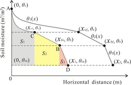
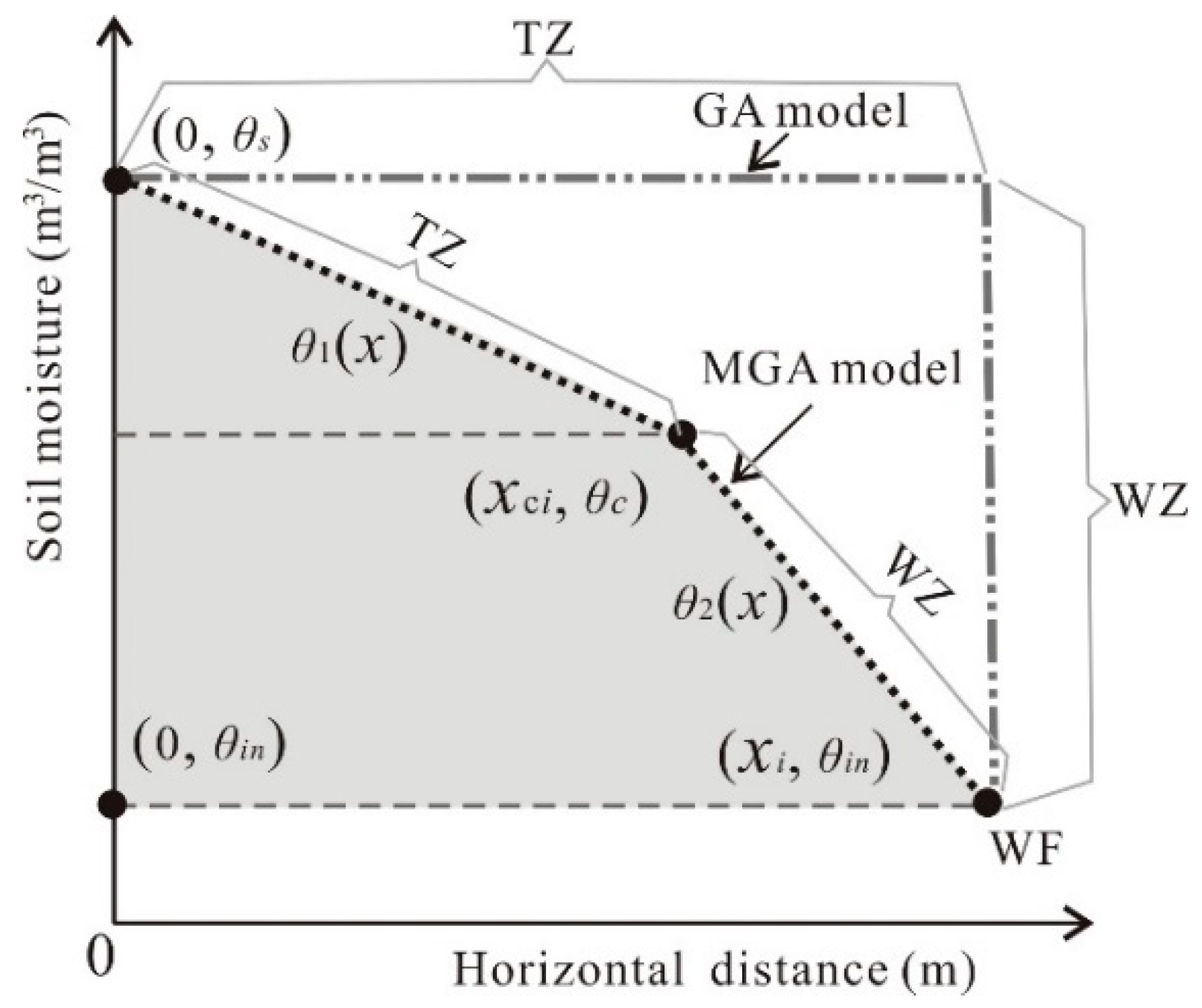
2. Improved Modified Green-Ampt Model

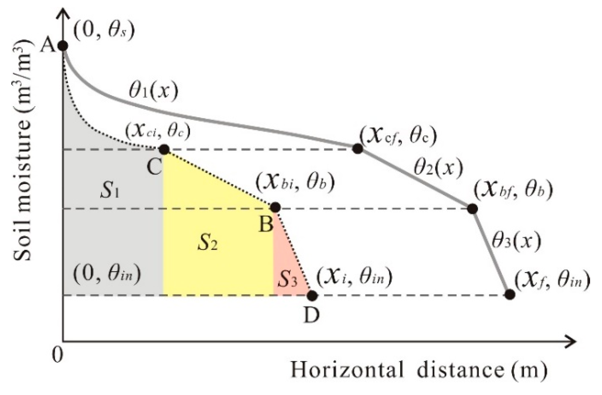
2.1. Theoretical Model Development

The GA model is based on the assumption that a rectangular piston moves into homogeneous isotropic soil with a uniform initial moisture content. It is assumed that there is a sharp WF in the soil that separates the soil moisture profile into a completely saturated zone and an unsaturated zone with initial moisture ${\theta }_{in}$. Mao et al. [35] modified these assumptions and used two linear functions, ${\theta }_1(x)$ and ${\theta }_2(x)$, to describe the soil moisture profiles in their MGA model, as seen in Figure 1.

As shown in Figure 1, the soil moisture profile function in the TZ, ${\theta }_1(x)$, is used to estimate the soil moisture profile shape of this zone which was defined by Prevedello et al. [29,30]. Soil moisture profile function, ${\theta }_2(x)$, is used to reflect the shape of the WZ. In the MGA model, it is assumed that after the WF, the soil moisture increase rate decreases linearly with distance of advance. This means that the matric suction after the WF, is determined by the soil particle surfaces and hypothetical constant capillary pores among the particles, which does not consider size changes of those particles. According to the theories introduced by Hillel [36] and Lu [37], water that exists in an unsaturated soil is subject to capillarity and adsorption, which combine to produce a matric suction $\psi$ (kPa), which can be described by the Laplace equation:

$$\psi =-\frac{2T_{\mathrm{s}}}{{\gamma }_{\mathrm{w}}{r}_{\mathrm{soil}}}$$

(1)

where $T_{\mathrm{s}}$ is surface tension of water (N/m²), $r_{\mathrm{soil}}$ is the radius of an idealized soil pore for fine soil (mm), and ${\gamma }_{\mathrm{w}}$ is the unit weight of water. Figure 2a shows that $r_{\mathrm{soil}}$ decreases with the growth of adsorbed water around soil particles, which causes $\psi$ and the rate of the saturation process to increase. Soils at different distances from the water supply, have different values of $r_{\mathrm{soil}}$—the closer to the water supply, the smaller the value of $r_{\mathrm{soil}}$. Therefore, to improve the MGA model, ${\theta }_1(x)$ should be redefined to take this effect into account. In addition, the data obtained by Prevedello et al. [29,30] indicate that the soil moisture profile in the WZ is not linear; it can be approximately fitted with two straight lines with different slopes. The ordinates of the intersections of these two lines are basically the same and are located in the moisture transition range.

In view of these observations, some improvements of the MGA model were made to transform the MGA model into the new IMGA model. Three functions, namely ${\theta }_1(x)$, ${\theta }_2(x)$, and ${\theta }_3(x)$, are used to describe the soil moisture profiles throughout the zones, as shown in Figure 3. In this figure, A, B, C, and D are the four points of inflection of the soil moisture profile. A logarithmic function is adopted to reflect the soil moisture change in the TZ (section AB in Figure 3):

$${\theta }_1(x)={\theta }_S-b\left(t\right)\ln (x+1)$$

(2)

where ${\theta }_S$ is saturated soil moisture (m³/m³) that is a constant for a specific soil, and $b(t)$ is a variable related to the elapsed time, which should be calibrated by lab tests. The cumulative infiltration can be estimated as [35]:

$$I=S_1+S_2+S_3$$

(3)

where $I$ is cumulative infiltration (mm). $S_1$, $S_2$, and $S_3$ can be further expressed as:

$$S_1=C_{tr}\left\{{\displaystyle {\int }_0^{x_c{}_i}\left[{\theta }_S-b(t)\ln (x+1)\right]}dx-{\theta }_{in}{x}_{ci}\right\}$$

(4)

$$S_2=\left(x_{bi}-x_{ci}\right)\left(\frac{{\theta }_b+{\theta }_c}{2}-{\theta }_{in}\right)$$

(5)

$$S_3=\frac{({\theta }_b-{\theta }_{in})(x_i-x_{bi})}{2}$$

(6)

where $C_{tr}$ is the unit transfer coefficient, which equals 1.509 here (the calculation process is introduced in Section 3.4). ${\theta }_c$ is critical soil moisture between TZ and WZ (m³/m³), ${\theta }_b$ is critical soil moisture between in the middle of WZ (m³/m³), ${\theta }_{in}$ is initial soil moisture (m³/m³), ${\theta }_1(x)$ is soil moisture profile function in the transmission zone (m³/m³), ${\theta }_2(x)$ soil moisture profile function in the WZ (m³/m³), $x_{ci}$ is advancement distance of the intersection point of two linear functions in the WZ and in the transmission zone (m), $x_{ci}$ is advancement distance of the intersection point of ${\theta }_1(x)$ and ${\theta }_2(x)$ (m), $x_{bi}$ is advancement distance of the intersection point of two linear functions in the WZ (m). The infiltration rate $m$ (mm/h) is defined as the derivative of $I$ with respect to time:

$$m=\frac{dI}{dt}$$

(7)

Prevedello et al. [29,30] proposed that the area of the WZ is constant during the infiltration process when elapsed time is large enough. Thus, the terms $(x_{bi}-x_{ci})$, $\left(\frac{{\theta }_b+{\theta }_c}{2}-{\theta }_{in}\right)$, $({\theta }_b-{\theta }_{in})$, and $(x_i-x_{bi})$ are constants. Equation (7) is further simplified as:

$$m=C_{tr}\frac{d}{dt}{\displaystyle {\int }_0^{x_{ci}}[{\theta }_S-b(t)\ln (x+1)]}dx-C_{tr}{\theta }_{in}\frac{d{x}_{ci}}{dt}$$

(8)

According to the Newton-Leibniz rule, Equation (8) can be rewritten as:

$$m=C_{tr}\frac{d{x}_{ci}}{dt}\left[{\theta }_S-b(t)\ln (x_{ci}+1)\right]+C_{tr}{\displaystyle {\int }_0^{x_{ci}}\left[-\frac{\partial b(t)}{\partial t}\ln (x_{ci}+1)\right]}-C_{tr}{\theta }_{in}\frac{d{x}_{ci}}{dt}$$

(9)

To compare the IMGA model with the GA and MGA models, the relationship between the advancement distance $x_{ci}$ and the elapsed time $t$ is expressed in the functional form that was used by Mao et al. [35]:

$$x_{ci}={\mathrm{k}}_1+{\mathrm{k}}_{2}t+{\mathrm{k}}_3{e}^{-{\mathrm{k}}_{4}t}$$

(10)

where ${\mathrm{k}}_1$, ${\mathrm{k}}_2$, ${\mathrm{k}}_3$, and ${\mathrm{k}}_4$ are constants related to soil properties and the water head difference, which should be calibrated by experiments. $b(t)$ denotes the soil moisture change rate in the TZ, which decrease with time. Here, a quadratic polynomial is suggested to be used to describe the relationship between $b(t)$ and $t$:

$$b(t)=-a{t}^2$$

(11)

where $a$ is a constant for a specific soil ($a$ > 0). Substituting Equations (11) and (10) into Equation (9) yields:

$$m_{\mathrm{IMGA}}=C_{tr}({\mathrm{k}}_2-{\mathrm{k}}_3{\mathrm{k}}_4{e}^{-{\mathrm{k}}_{4}t})\left[{\theta }_S-b(t)\ln (x_{ci}+1)-{\theta }_{in}\right]+C_{tr}{\displaystyle {\int }_0^{x_{ci}}\left[2at\ln (x_{ci}+1)\right]}d{x}_{ci}$$

(12)

The second term describes the influence of ${\theta }_1(x)$ change rate on the water infiltration rate, which is one magnitude less than the first term of Equation (12), so Equation (12) can be further simplified as:

$$m_{\mathrm{IMGA}}=C_{tr}({\mathrm{k}}_2-{\mathrm{k}}_3{\mathrm{k}}_4{e}^{-{\mathrm{k}}_{4}t})\left[{\theta }_S-b(t)\ln (x_{ci}+1)-{\theta }_{in}\right]$$

(13)

$$m_{\mathrm{MGA}}=C_{tr}\left(\frac{{\theta }_c+{\theta }_s}{2}-{\theta }_{in}\right)({\mathrm{k}}_2-{\mathrm{k}}_3{\mathrm{k}}_4{e}^{-{\mathrm{k}}_{4}t})$$

(14)

$$m_{\mathrm{GA}}=C_{tr}({\theta }_s-{\theta }_{in})({\mathrm{k}}_2-{\mathrm{k}}_3{\mathrm{k}}_4{e}^{-{\mathrm{k}}_{4}t})$$

(15)

Equations (13)–(15) are the relationships between the infiltration rate and the elapsed times estimated by the IMGA, MGA, and GA models, respectively.

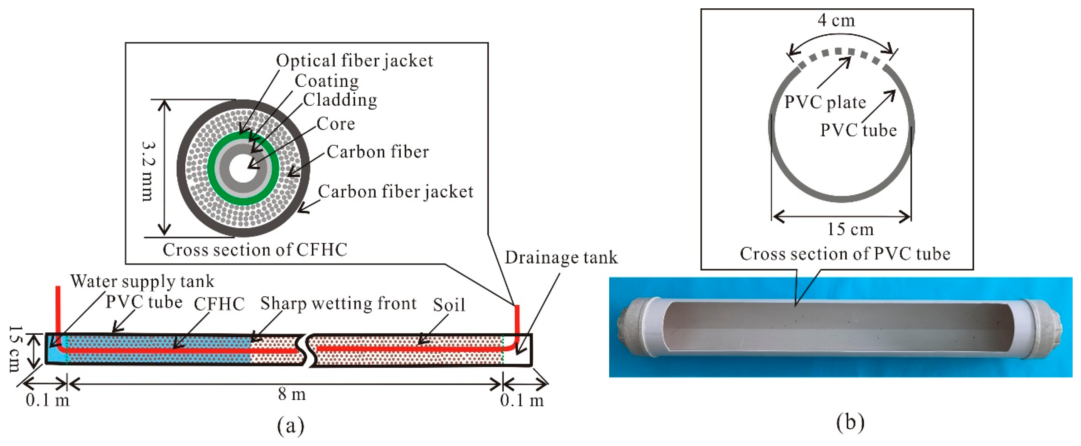
2.2. Setup of Calibration and Validation Tests

The horizontal infiltration tests were performed in a polyvinyl chloride (PVC) pipe. The pipe has a length of 8.2 m and an inner diameter of 15 cm, as shown in Figure 4. The PVC tube was divided into two sections by two filter papers that allow water to flow freely and prevent soil particles from passing through. The left space (with a length of 0.1 m) depicted in Figure 4 was a water tank for supplying water to the soil column during the following tests. The middle space with a length of 8 m was used for packing for soil samples. The right space with a length of 0.1 m was empty for draining. A piece of surface of the PVC pipe was removed, as shown in Figure 4b. Prior to testing, the soil samples were stirred by a shovel to make them homogeneous enough, and then backfilled into the tube. A carbon fiber heated cable (CFHC) was installed in the middle of the tube (Figure 4a). After all the soil samples were filled into the pipe, a transparent membrane was pasted on the ground surface to prevent water evaporation from soil and runoff on the soil surface. On the membrane, the removed PVC plate was covered by tape during the infiltration process.

During the tests, a distributed moisture sensing (DMS) interrogator (Model No. NZS–DMS–02, Suzhou NanZee Sensing Technology Co., Ltd, Suzhou, China) was used to automatically collect the soil moisture data. The primary performance parameters are shown in

Table 1. Basic parameters of the distributed moisture sensing (DMS) interrogator (NZS–DMS–M02).

Performance Parameters	Values
Distance measurement range (km)	0 to 50
Temperature measurement range (°C)	−40 to 120
Soil moisture measurement range (m3/m3)	0 to 0.65
Maximum current (A)	10
Fiber type	Multimode (50/125)
Moisture accuracy (m3/m3)	0.02
Response time (min)	20
Spatial resolution (m)	0.31
Sampling interval (m)	0.2
Channel number	2
Power consumption (W)	0 to 2000

. This interrogator has the integrated functions of heating the CFHC, measuring the distribution of temperature, deducing the soil moisture, and demonstrating the results. The working principle of this interrogator is based on the actively heated fiber optic (AHFO) method [38], which is suitable not only for laboratory experiments [38,39], but also for in situ tests [40,41,42,43]. Hence, the results measured with the AHFO method in these laboratory experiments can be compared with those in the field tests.

The soil used in the experiments was a mixture of quartz sand and kaolin at a mass ratio of 9:1. The initial soil moisture was 0.111 m³/m³ and the dry bulk density was 1.46 g/cm³. The initial soil moisture was the natural moisture content, which was determined by the air humidity and measured by the oven-drying method. The grain size distribution and soil water characteristic curve (SWCC) are shown in Figure 5 and Figure 6, respectively. The soil matric suctions under different soil moistures were measured using the filter paper method [44]. The SWCC was fitted using the Van Genuchten function [45].

During the test, under the pressure of the capillary force, the water in the left water supply tank entered the soil. The water supply tank was fully filled with water during the whole experiment, and the amount of water added to the water tank was recorded in real time. In general, the influence of water level on the horizontal infiltration is not considered. The horizontal infiltration experiments are often conducted in a liner tube that the influence of tube diameter can be neglected. Thus, the smaller the linear tube, the less the influence of the water level. In this study, the diameter (15 cm) is much smaller than the length of the soil column (8 m), thus, the impact of water tank size is not discussed. The soil moisture distribution was measured once every hour. The total time for every measurement is 20 min. The position of the WF was measured using a ruler with an accuracy of ±1 mm. The total period of each experiment was 24 h, and the soil moisture data were collected once per hour.

2.3. Parameter Determination Method

When determining soil moisture using the DMS, it is needed to calibrate the parameters. Soil moisture ($\theta$) was calculated according to the temperature characteristic value ($T_{\mathrm{t}}$), which was defined as the average temperature during a time period in the heating process [46]. Sayde et al. [38,47] suggested adopting a piecewise function to describe the relationship between $T_{\mathrm{t}}$ and $\theta$. In this study, if the soil moisture was larger than the threshold moisture (${\theta }_0$), a logarithmic function was used; otherwise, a linear function was adopted, as expressed in Equation (16):

$$T_{\mathrm{t}}=\{\begin{array}{l}{\mathrm{y}}_1-{\mathrm{y}}_2\ln (\theta +{\mathrm{y}}_3)\hspace{1em}\theta \ge {\theta }_0\\ {\mathrm{y}}_4\theta +{\mathrm{y}}_5\hspace{1em}\hspace{1em}\hspace{1em}\hspace{1em} \theta <{\theta }_0\end{array}$$

(16)

where ${\mathrm{y}}_1$, ${\mathrm{y}}_2$, ${\mathrm{y}}_3$, ${\mathrm{y}}_4$, and ${\mathrm{y}}_5$ are parameters determined by soil grain sizes, pore structure, composition, etc. In order to obtain these parameters, the actually measured soil moisture was measured by the oven-drying method via collected soil samples. The soil samples at different positions were collected every 30 min in the first four hours of the experiment. The relationship between $T_{\mathrm{t}}$ directly recorded by interrogator and $\theta$ was fitted using the least square method. Then, the soil moisture during the whole experiment was inferred from the calibrated relationship.

The constants in the functions ${\theta }_1(x)$, ${\theta }_2(x)$, and ${\theta }_3(x)$ were determined by the method of undetermined coefficients. After obtaining the actual measured soil moisture distribution by the DMS, the inflection points can be located through observation. ${\theta }_b$ and ${\theta }_c$ were the soil moisture of the inflection points. Thus the coordinates of the points A, B, C and D in Figure 3 could be determined. The slopes of lines BC and CD in Figure 3 could be calculated through the coordinates of the points A, B, C and D. The functions ${\theta }_1(x)$, ${\theta }_2(x)$, and ${\theta }_3(x)$ could be further determined using the method of undetermined coefficients. The calibration operation can be referred to [39].

2.4. Numerical Model

The theoretical soil moisture profile at any moment can be obtained by solving the Richards’ equation. In this study, only the horizontal mode is considered, which can be expressed as [37]:

$$\frac{\partial \theta }{\partial t}=\frac{\partial }{x}\left[D(\theta )\frac{\partial \theta }{\partial x}\right]$$

(17)

where $D(\theta )$ is the soil water diffusivity (m²/s), t is elapsed time (h), and $x$ is horizontal distance (m). The solution of Equation (17) is obtained by use of a finite element-based numerical method. The numerical model, which has the same size as the physical model in Figure 4, was built using the finite element method. The numerical model uses Richards’ equation as its governing equation. The unit grid is an equilateral triangle with a length of 0.015 m. The Brooks & Corey function and Van Genuchten function has been the most common models used in solving the Richards’ equation [45,48]. In this paper, the Van Genuchten function was selected. The parameters of the Van Genuchten function are listed in

Table 2. Parameter values for the van Genuchten model function.

Soil	Θs (m3/m3)	Θr (m3/m3)	A (1/m)	N	I	Ks (m/s)
Sand	0.41	0.055	7.5	1.89	0.5	6.379 × 10−4

, which are determined using the method that was introduced by Carsel & Parrish [49].

3. Results and Discussion

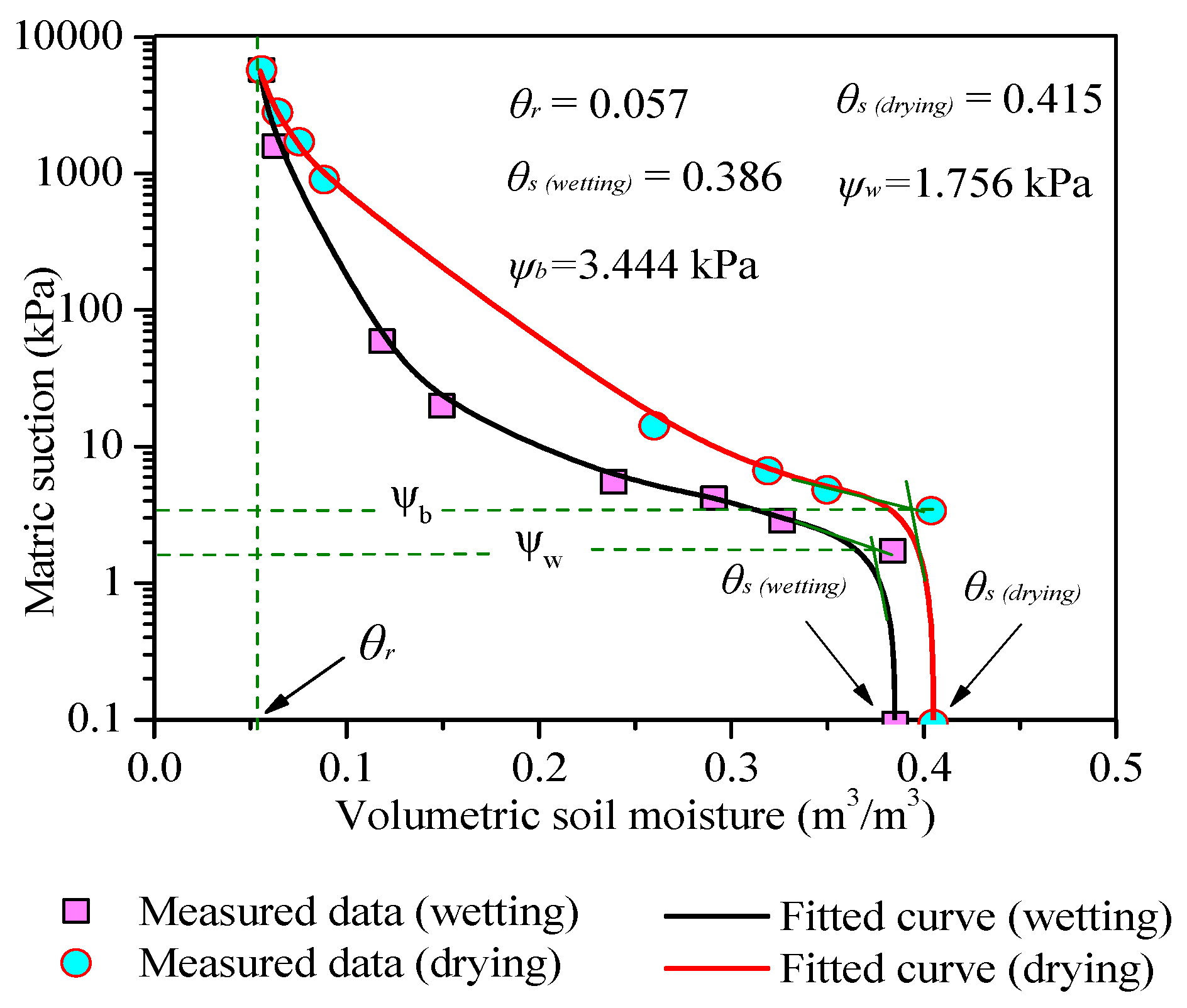
3.1. Parameters Calibration Results

The specific expression of Equation (16) were fitted as Equation (18) with an $R^2$ of 0.987:

$$T_{\mathrm{t}}=\{\begin{array}{l}7.476-1.656\ln (\theta +0.001)\hspace{1em}\hspace{1em}\hspace{1em}\theta >0.05\\ -203.916\theta +22.106\hspace{1em}\hspace{1em}\hspace{1em}\hspace{1em}\hspace{1em}\hspace{1em}\theta \le 0.05\end{array}$$

(18)

The horizontal soil moisture profiles at different infiltration moment were shown in Figure 7. The WZ during the first 2 h is not a constant that is not discussed in this study. Averaging the values of ${\theta }_b$ and ${\theta }_c$ that were measured during the period of 2–24 h in Figure 7 produced ${\theta }_b=0.25$ m³/m³ and ${\theta }_c=0.33$ m³/m³. The slopes of lines BC and CD in Figure 3 are ${\mathrm{k}}_{\mathrm{BC}}=0.09$ and ${\mathrm{k}}_{\mathrm{CD}}=0.35$ with R² of 0.987 and 0.975. ${\theta }_s$ and ${\theta }_{in}$ were obtained by the drying method; here, they are 0.42 m³/m³ and 0.11 m³/m³, respectively. It was further determined that $(x_{bi}-x_{ci})=1.5\mathrm{m}$, $(x_i-x_{bi})=0.4\mathrm{m}$, $\left(\frac{{\theta }_b+{\theta }_c}{2}-{\theta }_i\right)={0.19\mathrm{m}}^3{/\mathrm{m}}^3$, and $({\theta }_b-{\theta }_{in})={0.14\mathrm{m}}^3{/\mathrm{m}}^3$. The relationship between advancement distance of the wetting front and elapsed time is shown in Figure 8.

The parameters ${\mathrm{k}}_1$, ${\mathrm{k}}_2$, ${\mathrm{k}}_3$, and ${\mathrm{k}}_4$ in Equation (10) were fit using the least-squares method, as shown in Figure 8. The fitted result, with $R^2$ = 0.981, is expressed as:

$$x_{ci}=8.749-8.168e^{-0.084t}$$

(19)

It should be pointed out that only for the soil used in this study, ${\mathrm{k}}_2$ equals 0. The unit of hour is used for $t$. For the soil used in this study, by substituting ${\theta }_b=0.25$ m³/m³ and ${\theta }_c=0.33$ m³/m³ into Equation (2), the following expression is obtained:

$$b(t)=\frac{0.09}{\ln (1+8.749-8.168e^{-0.084t})}$$

(20)

According to Equation (15), ${\theta }_1(x)$ can be calculated at any moment. This means that the soil moisture profiles are only determined by $b(t)$ during this period.

3.2. Infiltration Rate

By substituting the parameters that were calibrated in Section 2.3 into Equations (13)–(15), the following expressions are obtained:

$$m_{\mathrm{IMGA}}=0.228e^{-0.084t}$$

(21)

$$m_{\mathrm{MGA}}=0.197e^{-0.084t}$$

(22)

$$m_{\mathrm{GA}}=0.321e^{-0.084t}.$$

(23)

Equations (21)–(23) indicate that, at any time, the infiltration rate estimated by the GA model is the largest, followed by those of the IMGA and MGA models. This is due to the difference in the assumed soil moisture profiles, as shown in Figure 9.

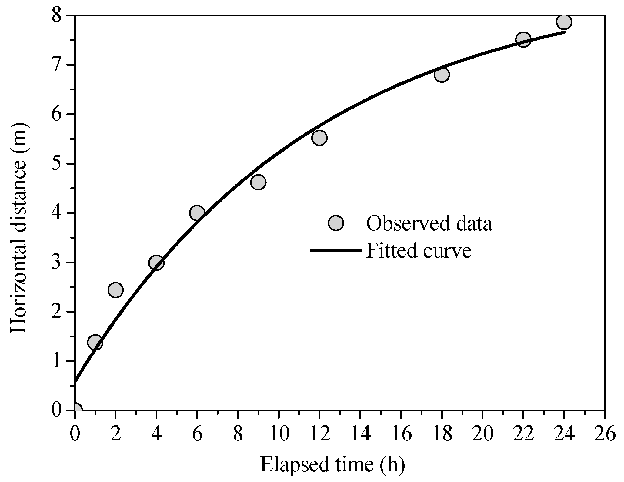
3.3. Cumulative Infiltration

Since the analytical integral process of Equation (8) is complicated and time consuming in applications, Equations (21)–(23) were directly integrated to obtain the cumulative infiltration in this study:

$$I_{\mathrm{IMGA}}=-2.714e^{-0.084t}+2.714$$

(24)

$$I_{\mathrm{MGA}}=-2.345e^{-0.084t}+2.345$$

(25)

$$I_{\mathrm{GA}}=-3.813e^{-0.084t}+3.813$$

(26)

Mao et al. [35] suggested that the error of the MGA model could be evaluated by comparing the predicted and actual values, but they did not specify which moment should be selected. To fill this gap, the predicted values of the IMGA, MGA, and GA models and the actual values that were measured using the graduated cylinder throughout the entire experimental process were selected, as shown in Figure 10.

It can be seen from Figure 10 that the deviations between the estimated cumulative infiltrations of the various models and the measured ones are different at different times. To quantify the deviation, the relative error ($\delta$), which was configured by Mao et al. [35], was used. It is defined as:

$$\delta =\left|\frac{V-IJ}{V}\right|\times 100\%$$

(27)

where $J$ is the cross-sectional area of the soil column (m²) packed by the PVC tube, $V$ is the total supplied water volume (m³/m³), and $\delta$ is the relative error. The comparison of $\delta$ among the IMGA, MGA, and GA models is shown in Figure 10.

Figure 10 shows that at the initial time, t = 0, the initial $\delta$ values for these models are very large. This is attributed to the weakness of this evaluation method. When the infiltration time is 0, the estimated cumulative infiltration is equal to 0 because the water has not flowed. However, it is necessary to add a certain amount of water to the tank to keep the water level at the required height. Therefore, there is a difference between the estimated and measured water volumes. When the elapsed time is larger than 0, the test periods can be divided into two stages: I and II, according to the relative error trend. The separation between these stages is at hour three. During the first stage, the relative errors of the three models decrease rapidly with time. During the second stage, for the GA model, $\delta$ increases with time, but for the MGA and IMGA models, it decreases with time. It can also be found that at any moment, $\delta$ of the IMGA model is less than that of the MGA model. Therefore, the elapsed time and experimental conditions should be considered when using the method proposed by Mao et al. [35] to evaluate the models’ accuracies.

Prevedello et al. [29,30] found that the TZ zone dominates the cumulative infiltration. The GA model assumes that the TZ is saturated at all times, which contradicts the actual measured values in Figure 7. Hence, with increased time, the differences between the GA model and the measured values accumulate, leading to increasingly large values of $\delta$. Both the MGA and IMGA models can precisely account for the true soil moisture change in the TZ. So, with increased time, the influence of the initial quantity of water that was added decreases. When calculating the infiltration rate and cumulative infiltration, the unit transfer coefficient is an essential parameter. Therefore, it is important to accurately determine this parameter.

3.4. Unit Transfer Coefficient $C_{tr}$

Mao et al. [35] took $C_{tr}$ = 10 in their study; however, they did not describe the specific calculation process of this parameter. $C_{tr}$ is determined by many factors, such as particle size, gradation, mineral composition, dry density, and model size. In this study, $C_{tr}$ was calibrated by laboratory experiments using the GA model. In the GA model, it is assumed that the TZ and WZ are saturated, so $C_{tr}$ can be calculated based on the mass conservation law. At moment $t$, the following holds:

$$\mathrm{J}x({\theta }_S-{\theta }_{in})=\mathrm{J}{I}_{\mathrm{GA}}$$

(28)

The general expressions of Equations (23) and (26) are:

$$I_{\mathrm{GA}}(t)=-\mathrm{E}{e}^{-0.084t}+\mathrm{E}$$

(29)

$$m_{\mathrm{GA}}(t)=\mathrm{F}{e}^{-0.084t}$$

(30)

where E and F are constants. Here, $t=24\mathrm{h}$ was taken as an example to illustrate the derivation process. It can be inferred from Equation (18) that $x_{ci}(24\mathrm{h})$ = 7.87 m. By substituting $x_{ci}(24\mathrm{h})$ = 7.87 m into Equations (29), it was found that E = 3.813, as shown in Equation (26). By calculating the different coefficients of Equation (30), it was found that F = 0.321, as shown in Equation (23). Equation (13) can be further rewritten as:

$$C_{tr}=\frac{m_{\mathrm{GA}}(t)}{[{\theta }_s-{\theta }_i{}_n](8.749-8.168e^{-0.084t})}$$

(31)

when $t$ = 24 h, it can be determined from Equation (31) that $i_{\mathrm{GA}}(24\mathrm{h})$ is 0.04275 mm. Considering that the term ${\theta }_s-{\theta }_{in}$ is a constant equal to 0.31 m³/m³, we obtained $C_{tr}$ = 1.509. $C_{tr}$ is an indicator of water driving force in TZ. According to the theories introduced by Hillel [36] and Lu [37], in the unsaturated soil without consideration of gravity, the driving force is soil suction. Thus, $C_{tr}$ is determined by many factors, such as absolute temperature, specific volume of water, water density, molecular mass of water vapor, partial pressure of pore-water vapor, saturation pressure of water vapor over a flat surface of pure water, pore structure, and grain size. In general, the smaller the soil particle is, the larger the $C_{tr}$ [36].

3.5. Moisture Profiles of Different Soils during the Infiltration Process

After investigating the infiltration characteristics of three soils, Mao et al. [35] found that different soils have different parameters in the MGA model. To verify the validity and reliability of the IMGA model in different soils, the data collected by Mao et al. [35] was fitted with the parameters of the IMGA model, as shown in Figure 11.

As shown in Figure 11, the results of the IMGA model (red curves) fit well with the measured data. Different soils have different line shapes with different parameters, as listed in

Table 3. Parameter values for different soils. BJ, AS and YL represent soil samples collected in Beijing, Ansai, and Yangling (China).

Soil Type		θs (m3/m3)	θc (m3/m3)	θb (m3/m3)	xi − xbi (cm)	xbi − xci (cm)	R2 (MGA)	R2 (IMGA)
Soil used in this test		0.416	0.332	0.253	39.57	149.62	0.834	0.927
Soils used by Mao	BJ	0.451	0.245	0.325	1.12	5.38	0.954	0.982
	AS	0.487	0.363	0.327	2.91	4.86	0.859	0.996
	YL	0.512	0.396	0.389	2.27	9.47	0.975	0.991

. It can be seen that for each soil, the R² of the IMGA model is larger than that of the MGA model, indicating that the former has a higher accuracy. The differences of the parameters among different soils suggest that these parameters should be calibrated for each soil.

3.6. Comparison between the IMGA Model and Solutions of Richards’ Equation

Both the IMGA model and Richards’ equation are physical models that describe horizontal infiltration of soil. To analyze and investigate their differences, the soil moisture profiles calculated by these two methods are shown in Figure 12.

As shown in Figure 12a, the numerical solutions of Richards’ equation do not conform to the measured values in two respects. First, the shapes of horizontal soil moisture profiles obtained by Richards’ equation and measured data are different. It can be distinctly pick out the TZ, WZ, and WF on the measured curves; however, the smooth simulation curves have no obvious demarcations (critical soil moisture), which is agrees well with the results of [50,51,52]. Mao et al. [35] and Herrada et al. [53] proposed that although the simplified numerical simulations can produce analytical solutions, they may lead to significant deviations from actually measured data. Second, the positions of the WF that were estimated by the numerical solutions of Richards’ equation differ from the observed positions. For the sake of analyzing the difference between these WF positions, a new variable $\Delta x$ (m) was used, which was defined as:

$$\Delta x=\left|x_{\mathrm{N}}-x_{\mathrm{M}}\right|$$

(32)

where $x_{\mathrm{N}}$ is the advancement distance is estimated by Richards’ equation (m) and $x_{\mathrm{M}}$ is the measured distance (m). Substituting $x_{\mathrm{N}}$ and $x_{\mathrm{M}}$, at the moments 2 h, 4 h, 6 h, 12 h, and 24 h into Equation (32) yields: $\Delta x(2\mathrm{h})=1.29\mathrm{m}$, $\Delta x(4\mathrm{h})=1.44\mathrm{m}$, $\Delta x(6\mathrm{h})=2.05\mathrm{m}$, $\Delta x(12\mathrm{h})=3.05\mathrm{m}$, and $\Delta x(24\mathrm{h})=4.02\mathrm{m}$.

Figure 12b shows that the soil profiles obtained by the IMGA model is closer than that of the simulated results of Richards equation. This is because when solving Richards’ equation, the Van Genuchten [45] function was used to describe the relationship between matric suction and moisture content. This function ascribes water infiltration to a matric suction imbalance without any consideration of the influence of gravity, pore size distribution, or interface. As a matter of fact, soils with different compositions, structures, and bulk densities have different SWCCs. In addition, it is difficult to ensure that the soil in the infiltration test is absolutely uniform and that the conditions in the infiltration test are the same as those under which the SWCC was measured. Mao et al. [35] also found that in porous soil, water tends to move in the direction of decreasing potential energy, and the gradient of potential energy with distance is the primary force of water flow. Therefore, various uncontrollable factors can cause the soil matric suction to change, and then lead to errors in the values predicted using Richards’ equation [54,55].

4. Conclusions

In this paper, the soil moisture profiles were measured by using actively heated fiber optic technology in laboratory, and some improvements have been made to the Green–Ampt (GA) and modified Green–Ampt (MGA) models. A new model, i.e., the improved modified Green–Ampt (IMGA) model, has been proposed to describe water infiltration in landslide dams. This model estimates the horizontal soil moisture profiles using three functions. A logarithmic function was used to reflect the soil moisture profile in the transition zone, and two linear functions were proposed for the wetting zone. The relationship between the advancement distance of the wetting front and time was fitted with an exponential function. After comparing and analyzing the IMGA, MGA, GA models, and the solutions of the Richards Equation, the following conclusions are drawn:

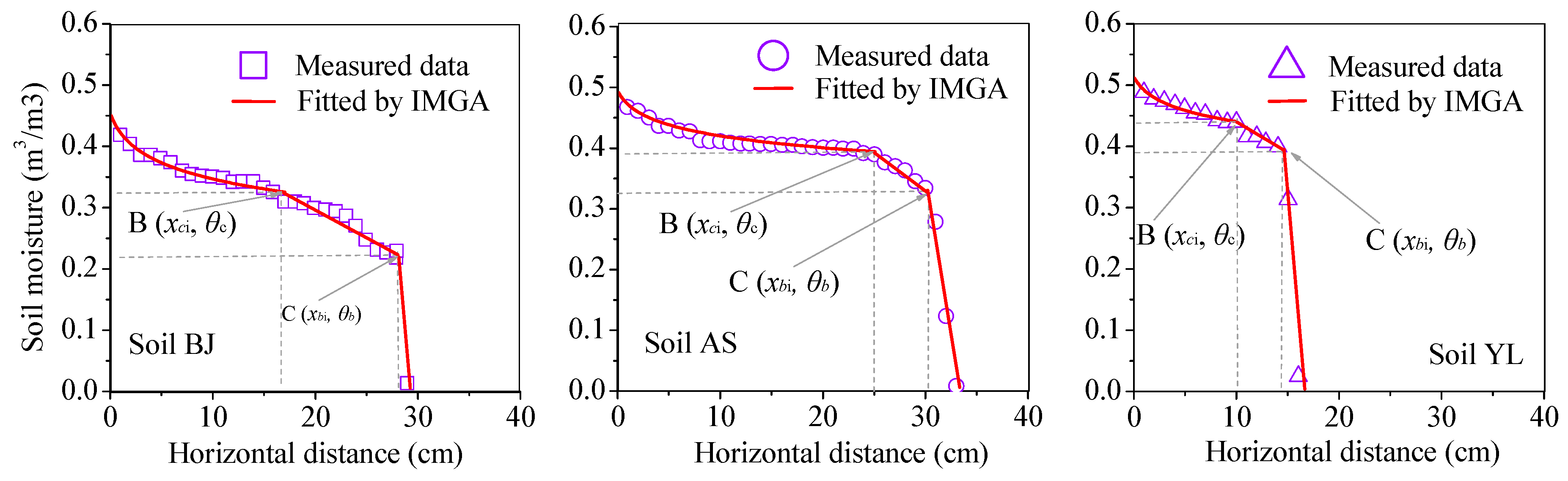
• The IMGA model enables accurate estimation of the soil moisture profile at any moment. The logarithmic function adopted by the IMGA model can capture changes in moisture content in the transition zone with a reflection of its decrease as the wetting front advances.
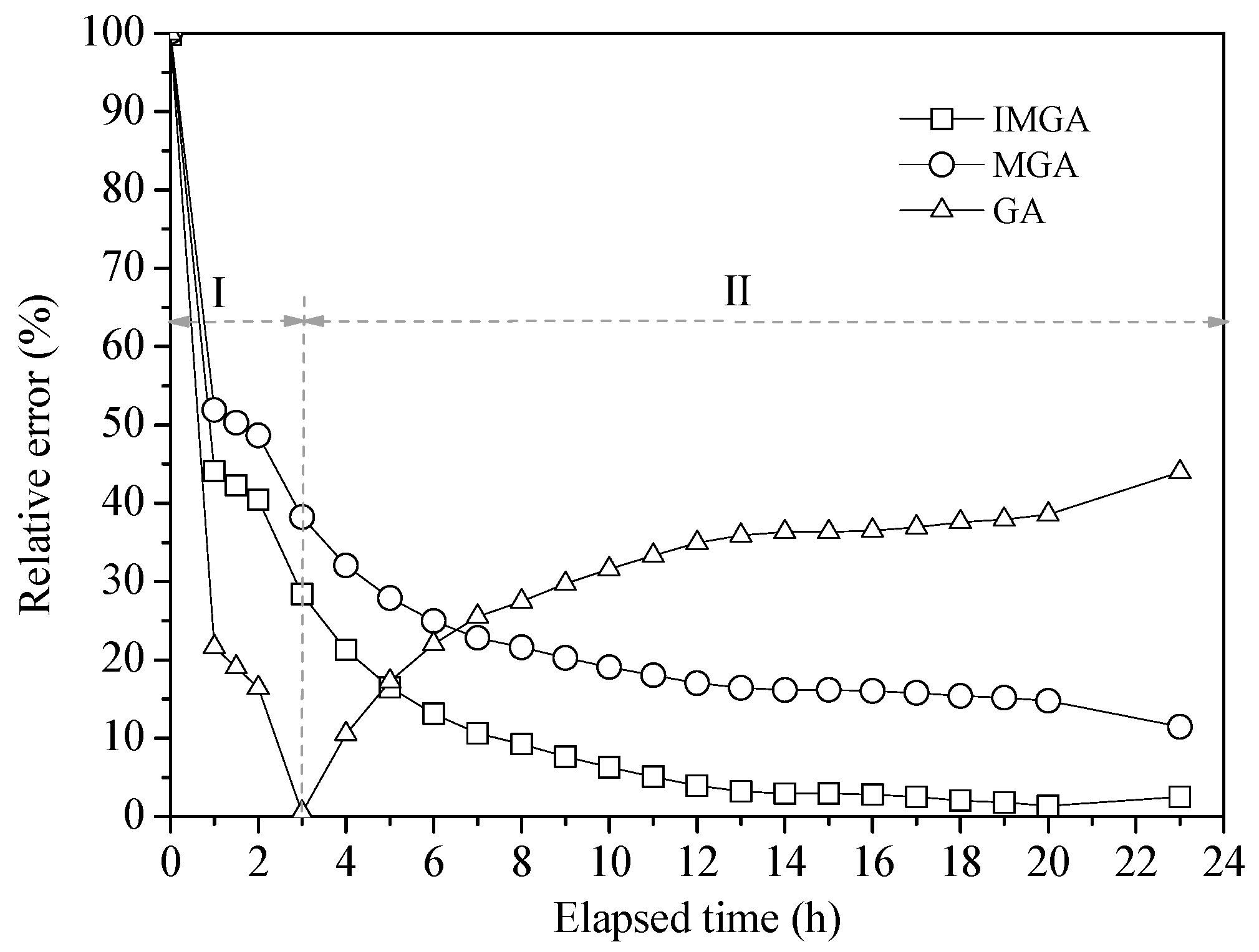
• By comparing the estimated cumulative infiltration data obtained using the models with those obtained by measurements, it was found that the IMGA model has the lowest relative error, followed by the MGA and GA models. It was also discovered that the relative errors of the models change with the infiltration time. The relative errors of the IMGA and MGA models monotonically decrease with time; however, for the GA model, the relative error first increases and then decreases. Therefore, the infiltration time should be specified when using this method to evaluate the errors of the models.
• It was demonstrated that the unit transfer coefficient $C_{tr}$ can be inferred from the GA model using the mass conservation law. Soils with different compositions, grain size and structures also have different $C_{tr}$ values, which can be determined by the method suggested in this study. The smaller the grain size, the larger $C_{tr}$ is.
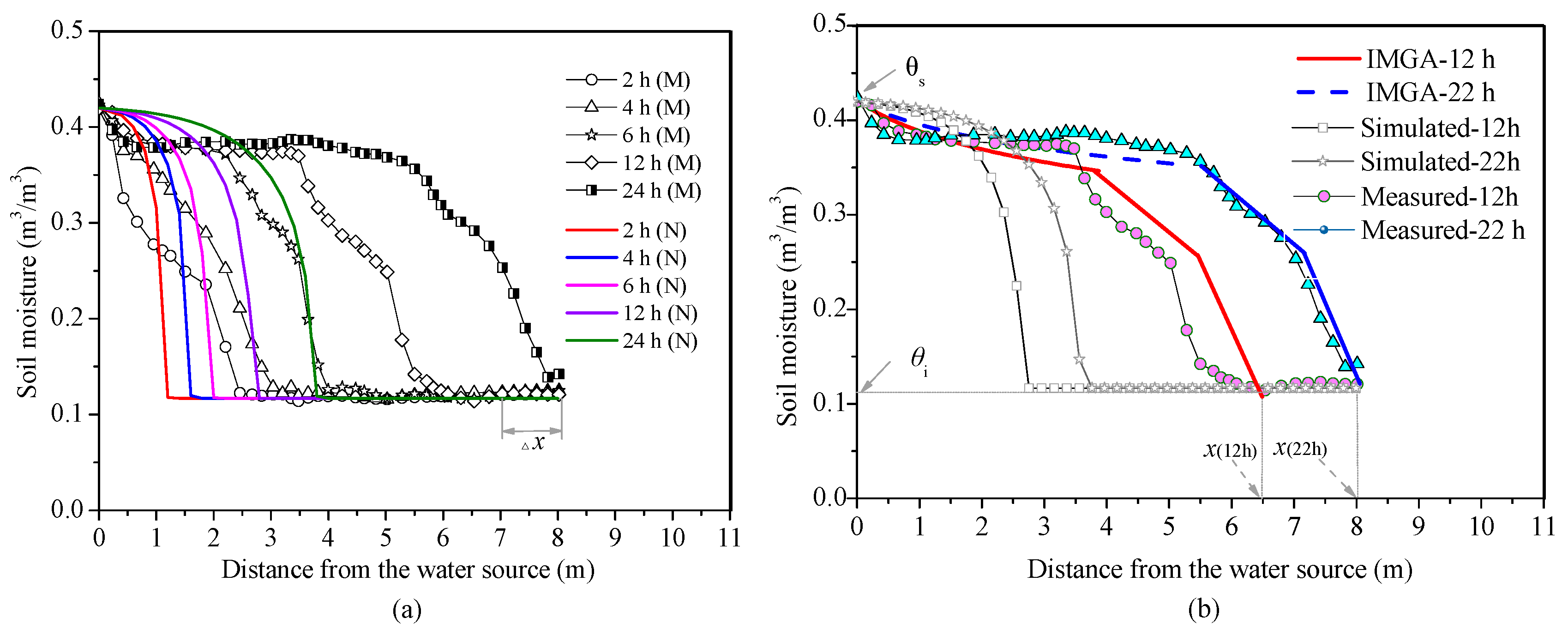
• Due to the unavoidable influence of interfaces and inhomogeneity in soil, the advancement distance of water infiltration calculated using Richards’ equation is shorter than that estimated by the IMGA model and the measured values. Another feature of the numerical solutions of Richards’ equation is that it is unable to reflect transmission zone, wetting zone, and demarcation point between these two zones. The horizontal soil moisture profiles obtained by the IMGA model is closer to the measured data than that of the numerical simulation results.

Although the IMGA model enables an accurate description of the horizontal soil moisture profiles during an infiltration process, similar to the MGA and GA models, there are still some deficiencies that limit its further application. For example, it cannot predict the infiltration in heterogeneous soil, which exists extensively in nature, or estimate two- or three-dimensional soil moisture profiles.

References

1. Song, Y.; Lu, Y.; Guo, Z.; Xu, X.; Liu, T.; Wang, J.; Wang, W.J.; Hao, W.J. Variations in Soil Water Content and Evapotranspiration in Relation to Precipitation Pulses within Desert Steppe in Inner Mongolia, China. Water 2019, 11, 198. [Google Scholar] [CrossRef]
2. Vidana Gamage, D.N.; Biswas, A.; Strachan, I.B. Field Water Balance Closure with Actively Heated Fiber-Optics and Point-Based Soil Water Sensors. Water 2019, 11, 135. [Google Scholar] [CrossRef]
3. De Almeida, W.S.; Panachuki, E.; De Oliveira, P.T.S.; Da Silva Menezes, R.; Sobrinho, T.A.; De Carvalho, D.F. Effect of soil tillage and vegetal cover on soil water infiltration. Soil Tillage Res. 2018, 175, 130–138. [Google Scholar] [CrossRef]
4. Liu, Z.; Ma, D.; Hu, W.; Li, X. Land use dependent variation of soil water infiltration characteristics and their scale-specific controls. Soil Tillage Res. 2018, 178, 139–149. [Google Scholar] [CrossRef]
5. Cheik, S.; Bottinelli, N.; Soudan, B.; Harit, A.; Chaudhary, E.; Sukumar, R.; Jouquet, P. Effects of termite foraging activity on topsoil physical properties and water infiltration in Vertisol. Appl. Soil Ecol. 2019, 133, 132–137. [Google Scholar] [CrossRef]
6. Weller, U.; Leuther, F.; Schlüter, S.; Vogel, H.J. Quantitative analysis of water infiltration in soil cores using x-ray. Vadose Zone J. 2018, 17, 17. [Google Scholar] [CrossRef]
7. Toro-Guerrero, D.; Vivoni, E.; Kretzschmar, T.; Bullock Runquist, S.; Vázquez-González, R. Variations in Soil Water Content, Infiltration and Potential Recharge at Three Sites in a Mediterranean Mountainous Region of Baja California, Mexico. Water 2018, 10, 1844. [Google Scholar] [CrossRef]
8. Yeh, H.F.; Tsai, Y.J. Effect of Variations in Long-Duration Rainfall Intensity on Unsaturated Slope Stability. Water 2018, 10, 479. [Google Scholar] [CrossRef]
9. Mishra, S.K.; Tyagi, J.V.; Singh, V.P. Comparison of infiltration models. Hydrol. Processes 2003, 17, 2629–2652. [Google Scholar] [CrossRef]
10. Cho, S.E.; Lee, S.R. Evaluation of surficial stability for homogeneous slopes considering rainfall characteristics. J. Geotech. Geoenviron. Eng. 2002, 128, 756–763. [Google Scholar] [CrossRef]
11. Prevedello, C.L.; Loyola, J.M.T.; Reichardt, K.; Nielsen, D. New Analytic Solution Related to the Richards, Philip, and Green–Ampt Equations for Infiltration. Vadose Zone J. 2009, 8, 127–135. [Google Scholar] [CrossRef]
12. Al–Maktoumi, A.; Kacimov, A.; Al–Ismaily, S.; Al-Busaidi, H.; Al-Saqri, S. Infiltration into Two–Layered Soil: The Green–Ampt and Averyanov Models Revisited. Transp. Porous Media 2015, 109, 169–193. [Google Scholar] [CrossRef]
13. Zaibon, S.; Anderson, S.H.; Thompson, A.L.; Thompson, A.L.; Kitchen, N.R.; Gantzer, C.J.; Haruna, S.I. Soil water infiltration affected by topsoil thickness in row crop and switchgrass production systems. Geoderma 2017, 286, 46–53. [Google Scholar] [CrossRef]
14. Ojha, R.; Corradini, C.; Morbidelli, R.; Govindaraju, R.S. Effective saturated hydraulic conductivity for representing field–scale infiltration and surface soil moisture in heterogeneous unsaturated soils subjected to rainfall events. Water 2017, 9, 134. [Google Scholar] [CrossRef]
15. Stewart, R.D. A Dynamic Multidomain Green-Ampt Infiltration Model. Water Resour. Res. 2018, 54, 6844–6859. [Google Scholar] [CrossRef]
16. Baiamonte, G.; Singh, V.P. Analytical solution of kinematic wave time of concentration for overland flow under Green–Ampt infiltration. J. Hydrol. Eng. 2015, 21, 04015072. [Google Scholar] [CrossRef]
17. Grimaldi, S.; Petroselli, A.; Romano, N. Green-Ampt Curve-Number mixed procedure as an empirical tool for rainfall–runoff modelling in small and ungauged basins. Hydrol. Processes 2013, 27, 1253–1264. [Google Scholar] [CrossRef]
18. Ma, D.; Zhang, J.; Lu, Y.; Wu, L.S.; Wang, Q. Derivation of the Relationships between Green–Ampt Model Parameters and Soil Hydraulic Properties. Soil Sci. Soc. Am. J. 2015, 79, 1030–1042. [Google Scholar] [CrossRef]
19. Zema, D.A.; Labate, A.; Martino, D.; Zimbone, S.M. Comparing Different Infiltration Methods of the HEC–HMS Model: The Case Study of the Mésima Torrent (Southern Italy). Land Degrad. Dev. 2017, 28, 294–308. [Google Scholar] [CrossRef]
20. Bouvier, C.; Bouchenaki, L.; Tramblay, Y. Comparison of SCS and Green-Ampt Distributed Models for Flood Modelling in a Small Cultivated Catchment in Senegal. Geosciences 2018, 8, 122. [Google Scholar] [CrossRef]
21. Almedeij, J.; Esen, I.I. Modified Green–Ampt infiltration model for steady rainfall. J. Hydraul. Eng. 2014, 19, 0401410. [Google Scholar] [CrossRef]
22. Tang, J.L.; Cheng, X.Q.; Zhu, B.; Gao, M.; Wang, T.; Zhang, X.; Zhao, P.; You, X. Rainfall and tillage impacts on soil erosion of sloping cropland with subtropical monsoon climate—a case study in central Sichuan Basin, China. J. Mt. Sci. 2015, 12, 134–144. [Google Scholar] [CrossRef]
23. Xiang, L.; Ling, W.; Zhu, Y.; Chen, L.; Yu, Z. Self–adaptive Green–Ampt infiltration parameters obtained from measured moisture processes. Water Sci. Eng. 2016, 9, 256–264. [Google Scholar] [CrossRef]
24. Deng, P.; Zhu, J. Analysis of effective Green–Ampt hydraulic parameters for vertically layered soils. J. Hydrol. 2016, 538, 705–712. [Google Scholar] [CrossRef]
25. Chen, L.; Xiang, L.; Young, M.H.; Yin, Y.; Yu, Z.; Van Genuchten, M. Optimal parameters for the Green–Ampt infiltration model under rainfall conditions. J. Hydrol. Hydromech. 2015, 63, 93–101. [Google Scholar] [CrossRef]
26. Ali, S.; Islam, A. Solution to Green–Ampt infiltration model using a two-step curve-fitting approach. Environ. Earth Sci. 2018, 77, 271. [Google Scholar] [CrossRef]
27. Wu, S.; Shi, L.; Wang, R.; Tan, C.; Hu, D.; Mei, Y.; Xu, R. Zonation of the landslide hazards in the forereservoir region of the Three Gorges Project on the Yangtze River. Eng. Geol. 2001, 59, 51–58. [Google Scholar] [CrossRef]
28. Kale, R.V.; Sahoo, B. Green–Ampt infiltration models for varied field conditions: A revisit. Water Resour. Manag. 2011, 25, 3505–3536. [Google Scholar] [CrossRef]
29. Prevedello, C.L.; Loyola, J.M.; Reichardt, K.; Donald, N. New analytic solution of Boltzmann transform for horizontal water infiltration into sand. Vadose Zone J. 2008, 7, 1170–1177. [Google Scholar] [CrossRef]
30. Prevedello, C.L.; Armindo, R.A. Generalization of the Green–Ampt Theory for Horizontal Infiltration into Homogeneous Soils. Vadose Zone J. 2016, 15, 1–10. [Google Scholar] [CrossRef]
31. Philip, J.R. Numerical solution of equations of the diffusion type with diffusivity concentration–dependent. Trans. Faraday Soc. 1955, 51, 885–892. [Google Scholar] [CrossRef]
32. Philip, J.R. Numerical Solution of Equations of the Diffusion Type with Diffusivity Concentration–Dependent II. Aust. J. Phys. 1957, 10, 29–42. [Google Scholar] [CrossRef]
33. Barry, D.A.; Parlange, J.Y.; Prevedello, C.L.; Loyola, J.M.T. Extension of a recent method for obtaining exact solutions of the Bruce and Klute equation. Vadose Zone J. 2010, 9, 496–498. [Google Scholar] [CrossRef]
34. Green, W.H.; Ampt, G.A. Studies on Soil Phyics. J. Agric. Sci. 1911, 4, 1–24. [Google Scholar] [CrossRef]
35. Mao, L.; Li, Y.; Hao, W.; Zhou, X.; Xu, C.; Lei, T. A new method to estimate soil water infiltration based on a modified Green–Ampt model. Soil Tillage Res. 2016, 161, 31–37. [Google Scholar] [CrossRef]
36. Hillel, D. Introduction to Environmental Soil Physics; Elsevier Academic Press: Amsterdam, The Netherlands, 2004; p. 110. [Google Scholar]
37. Lu, N.; Godt, J.W. Hillslope Hydrology and Stability; Cambridge University Press: Cambridge, UK, 2013; p. 91. [Google Scholar]
38. Sayde, C.; Gregory, C.; Gil-Rodriguez, M.; Tufillaro, N.; Tyler, S.; Van de Giesen, N.; English, M.; Cuenca, R.; Selker, J.S. Feasibility of soil moisture monitoring with heated fiber optics. Water Resour. Res. 2010, 46, 2840–2849. [Google Scholar] [CrossRef]
39. Cao, D.F.; Shi, B.; Zhu, H.H.; Zhu, K.; Wei, G.Q.; Gu, K. Performance evaluation of two types of heated cables for distributed temperature sensing–based measurement of soil moisture content. J. Rock Mech. Geotech. Eng. 2016, 8, 212–217. [Google Scholar] [CrossRef]
40. Sourbeer, J.J.; Loheide, S.P. Obstacles to long-term soil moisture monitoring with heated distributed temperature sensing. Hydrol. Processes 2016, 30, 1017–1035. [Google Scholar] [CrossRef]
41. Benítez-Buelga, J.; Rodríguez-Sinobas, L.; Sánchez Calvo, R.; Gil-Rodríguez, M.; Sayde, C.; Selker, J.S. Calibration of soil moisture sensing with subsurface heated fiber optics using numerical simulation. Water Resour. Res. 2016, 52, 2985–2995. [Google Scholar] [CrossRef]
42. Su, H.; Tian, S.; Cui, S.; Yang, M.; Wen, Z.; Xie, M. Distributed optical fiber-based theoretical and empirical methods monitoring hydraulic engineering subjected to seepage velocity. Opt. Fiber Technol. 2016, 31, 111–125. [Google Scholar] [CrossRef]
43. Su, H.; Tian, S.; Kang, Y.; Xie, W. Monitoring water seepage velocity in dikes using distributed optical fiber temperature sensors. Autom. Constr. 2017, 76, 71–84. [Google Scholar] [CrossRef]
44. Bai, F.Q.; Liu, S.H.; Yuan, J. Measurement of SWCC of Nanyang expansive soil using the filter paper method. Chin. J. Geotech. Eng. 2011, 33, 928–933. (In Chinese) [Google Scholar]
45. Van Genuchten, M.T. A closed–form equation for predicting the hydraulic conductivity of unsaturated soils. Soil Sci. Soc. Am. J. 1980, 44, 892–898. [Google Scholar] [CrossRef]
46. Cao, D.; Shi, B.; Zhu, H.; Wei, G.; Chen, S.; Yan, J. A distributed measurement method for in-situ soil moisture content by using carbon-fiber heated cable. J. Rock Mech. Geotech. Eng. 2015, 7, 700–707. [Google Scholar] [CrossRef] [Green Version]
47. Sayde, C.; Buelga, J.B.; Rodriguez-Sinobas, L.; Khoury, L.; English, M.; van de Giesen, N.; Selker, J.S. Mapping variability of soil water content and flux across 1–1000 m scales using the actively heated fiber optic method. Water Resour. Res. 2014, 50, 7302–7317. [Google Scholar] [CrossRef]
48. Brooks, R.H.; Corey, A.T. Hydraulic properties of porous media and their relation to drainage design. Trans. ASAE 1964, 7, 26–28. [Google Scholar]
49. Carsel, R.F.; Parrish, R.S. Developing joint probability distributions of soil water retention characteristics. Water Resour. Res. 1988, 24, 755–769. [Google Scholar] [CrossRef]
50. Pachepsky, Y.; Timlin, D.; Rawls, W. Generalized Richards’ equation to simulate water transport in unsaturated soils. J. Hydrol. 2003, 272, 3–13. [Google Scholar] [CrossRef]
51. Płociniczak, Ł. Analytical studies of a time-fractional porous medium equation. Derivation, approximation and applications. Commun. Nonlinear Sci. Numer. Simul. 2015, 24, 169–183. [Google Scholar] [CrossRef] [Green Version]
52. Xiao, H.; Huang, J. Experimental study of the applications of fiber optic distributed temperature sensors in detecting seepage in soils. Geotech. Test. J. 2013, 36, 360–368. [Google Scholar] [CrossRef]
53. Herrada, M.A.; Gutiérrez-Martin, A.; Montanero, J.M. Modeling infiltration rates in a saturated/unsaturated soil under the free draining condition. J. Hydrol. 2014, 515, 10–15. [Google Scholar] [CrossRef]
54. Leong, E.C.; Rahardjo, H. Review of soil–water characteristic curve equations. J. Geotech. Geoenviron. Eng. 1997, 123, 1106–1117. [Google Scholar] [CrossRef]
55. Likos, W.J.; Lu, N.; Godt, J.W. Hysteresis and uncertainty in soil water–retention curve parameters. J. Geotech. Geoenviron. Eng. 2013, 140, 1–11. [Google Scholar] [CrossRef]
Figure 1. Assumed soil moisture profiles in the Green–Ampt (GA) and modified Green–Ampt (MGA) models. θ S is saturated soil moisture (m3/m3), θ c is critical soil moisture between transmission zone (TZ) and wetting zone (WZ) (m3/m3), θ i n is initial soil moisture (m3/m3), θ 1 ( x ) is soil moisture profile function in the transmission zone (m3/m3), θ 2 ( x ) soil moisture profile function connected with TZ in the wetting zone (m3/m3), x c i is advancement distance of the intersection point of two linear functions in the wetting zone and in the transmission zone (m), x i is advancement distance of the WF (m), TZ is transmission zone, WZ is wetting zone, WF is wetting front, and i means a moment during the infiltration process.
Water 11 00645 g001
Figure 2. Water in an unsaturated soil: (a) actual soil moisture distribution introduced by Hillel [36] after a wetting front; (b) soil moisture distribution described by the GA model; and (c) soil moisture distribution described by the MGA model.
Water 11 00645 g002
Figure 3. Soil moisture profiles simulated with the improved modified Green–Ampt (IMGA) model over time (the dashed line is the soil moisture profile at time i, and the solid line is the moisture profile at a later time f). θ b is critical soil moisture in the middle of WZ (m3/m3), θ 3 ( x ) is soil moisture profile function connected with WF in the wetting zone (m3/m3), x b i is advancement distance of the point of intersection of two linear functions in the wetting zone (m).
Water 11 00645 g003
Figure 4. Configuration of the experimental apparatus: (a) soil column and cross section of the carbon fiber heated cable (CFHC); (b) cut region of the polyvinyl chloride (PVC) tube.
Water 11 00645 g004
Figure 5. Soil grain size distribution.
Water 11 00645 g005
Figure 6. Soil water characteristic curves for the soil samples. θ S   ( d r y i n g ) and θ S   ( w e t t i n g ) are the saturated soil moistures under drying and wetting paths (m3/m3), respectively; θ r is the residual moisture (m3/m3); ψ b is the air entry pressure (kPa); and ψ w is the water entry pressure (kPa).
Water 11 00645 g006
Figure 7. Soil moisture profiles measured by the DMS interrogator. θ c zone is the soil moisture range θ c located in, and θ b zone is the soil moisture range θ b located in.
Water 11 00645 g007
Figure 8. Advancement distance of the wetting front with elapsed time.
Water 11 00645 g008
Figure 9. Water infiltration rates estimated by the IMGA, MGA, and GA models.
Water 11 00645 g009
Figure 10. Relative errors of the IMGA, MGA, and GA models as a function of time. I is the period in which the error of GA model degreases. II is the period in which the error of GA model increases.
Water 11 00645 g010
Figure 11. Soil moisture profiles measured by Mao et al. [35] and the fit results of the IMGA model. BJ, AS and YL represent soil samples collected in Beijing, Ansai, and Yangling (China), respectively.
Water 11 00645 g011
Figure 12. Soil moisture profile comparison: (a) wetting front comparison between actually measured values (M) and numerical solutions (N) of Richards’ equation, and (b) soil moisture profile comparison among the IMGA model, solutions of Richards’ equation and actually measured values.
Water 11 00645 g012