Non-Negligible Lag of Groundwater Infiltration Recharge: A Case in Mu Us Sandy Land, China

Abstract

Groundwater is often the main source of available water, and precipitation is one of the main recharge sources of groundwater in arid and semi-arid regions. This paper studies a fixed dune in Mu Us Sandy Land in China, establishes a numerical model, acquires hydraulic parameters and heat parameters of the vadose zone, and calculates the recharge coefficient based on field observation data and numerical modelling. These measurement results show that the response depths of storm rain are more than 90 cm, while those of small rain events are less than 10 cm. The numerical results show that infiltration depths are 10 cm for small rain and more than 90 cm for middle rain respectively. The lag time of the water content at 90 cm below the surface was 25 h following a middle rain, 18–19 h following a heavy rain, and 16–18 h following a storm rainfall. Groundwater recharge lag times (matrix flow) varied from 11 h to 48 h. Excluded precipitation for groundwater recharge was 11.25–11.75 mm in 1 h when groundwater depth was 120 cm and 15–15.5 mm when 140 cm, showing significant influence in groundwater resource evaluation.

1. Introduction

Precipitation infiltration recharge rates are important for identifying balanced components of groundwater, especially in semi-arid regions where surface water is scarce. It is affected by the groundwater depth, lithology of vadose zone, precipitation characteristics, atmospheric conditions [1], and by human factors such as land use and land cover. Groundwater recharge and its relationship with precipitation input has been a hot topic among researchers for a long time [2,3,4,5]. At present, there are many methods to estimate the precipitation recharge. Calculating the water flux based on observed water content, pressure head was widely used in the past. However, due to the different lithology of the vadose zone and preference flows, groundwater recharge varies greatly among different regions. Thus, point monitoring results are not representative at the regional scale [6,7]. Simultaneously, observed data are also affected by the specific conditions in the field [8]. Therefore, numerical simulations have been accepted in the calculation of recharge in the vadose zone and saturated zone [9,10,11].

Due to high evaporation and dry climates in semi-arid regions, water content in the vadose zone only responds to large precipitation and the recharge coefficients of precipitation (amount of groundwater recharge divided by precipitation) are often smaller than in humid regions. Only precipitation of more than 20 mm can effectively recharge groundwater in the Dunhuang desert regions of China [12]. Precipitation of less than 30 mm cannot form effective recharge to groundwater in the Badan Jilin Desert in China [13]. In the semi-arid area of the Eastern Mediterranean Seas, the recharge coefficient of precipitation is 0.29 in bare dunes, and 0.01 in dunes with high coverage [14].

Scarce surface water resources, dry climate, and development of industry and agriculture all contribute to a severe problem of groundwater use. It is critical to improve the accuracy of groundwater resource evaluation in semi-arid regions. Previous studies often calculated groundwater recharge resources by annual precipitation and distributed recharge coefficients of precipitation (α) in regional groundwater research [5,15,16]. However, heterogeneous lithology of the soil vadose zone frequently complicates this recharge process. Recharge at water table always lags behind precipitation due to the unsaturated flow rate, clearly predicting that recharge is not determined directly by the precipitation in that period but precipitation in another earlier period of equal length [17,18,19,20]. Therefore, it is important to determine the lag time between the input elements and responses of aquifers in order to improve the accuracy of precipitation recharge calculations, especially in semi-arid regions where recharge lag is obvious and annual precipitation varies greatly. Also, considering the lag time of groundwater recharge can significantly improve the accuracy of groundwater flow models [21,22].

The vadose zone, the only way that precipitation recharge must pass through, is an important part of Earth’s critical zone. In many part of the world, land-use intensification, global climate change, and mineral exploitation are changing vadose zones directly, and then effecting groundwater retention systems [23]. Irrigation using groundwater in arid and semi-arid regions reduces the water table and vertical recharge [24]. Compared with natural grass land, planted agricultural crops significantly increase soil water volume, promoting deep drainage and groundwater recharge [10]. Furthermore urbanization and agriculture fertilization also contribute to the contamination or quality change in vadose zones and groundwater [25,26,27].

When considering groundwater recharge lag, changes in groundwater recharge and water quality are essential for most accurate modeling the direct and indirect effects of precipitation rates on groundwater modifications. It was found that the response time of changes in groundwater recharge can reach 200 y after turning natural land into non-irrigated crop land in the arid areas of Niger [10]. The response time of soil drainage change is greater than 50 y in the vertisol zone of Australia [28,29]. Also, groundwater recharge lag time may be less than 100 days in some area of Australia and Brazil resulting in bypass flow or shallow groundwater depth [30,31]. Damage effects to aquifers caused by surface environmental change and human activities is often hard to detect in the short term. Determining groundwater recharge lag time more accurately can help to analyze the impact of human activities and climate change on groundwater quality and quantity and promote sustainable development of water resource use [10,23].

By means of piezometers and observation wells, lag times were determined about 2–20 h in very shallow groundwater areas of fine-textured soils in Kansas (0–4 m) and central Missouri (2–3 m) [22,32]. Due to the quite low conductivities, the groundwater recharge lag time was about 28–173 days in shallow depth areas of the Naoli River Basin [33]. These works suggest that soil structure and soil media all effect the recharge of groundwater. But their work ignored variations in the infiltration and flow through the vadose zones modified by time intervals of measurement and field conditions. In the past, there was little consideration for the time lag of precipitation infiltration recharge in shallow groundwater regions. Recently, significant lagging recharge in shallow groundwater areas (1–1.5 m depth) of Mu Us Sandy Land was reported [34]. A range of 3–30 years of groundwater ages in shallow groundwater areas of Memphis, TN was determined, showing obvious mixing effects in the vadose zone [35], resulting in calculation errors of recharge lag time.

Although the lag time of precipitation recharge in semi-arid regions is often at the scale of days, it cannot be ignored due to the extremely high-water dependence and requirement of accurate evaluation of groundwater resources. In Mu Us Sandy Land, where groundwater depth is often shallow (1–4 m), the areas with groundwater depths of 1–1.5 m account for about 15% of the full Mu Us Sandy Land, and the surface water resources are extremely scarce and groundwater is highly utilized [36]. With the continuous development of the energy industry in this region, the increasing water consumption has created severe challenges for the relatively fragile hydrological ecology. Also, the northwest of China has experienced a substantial changes in surface cover since 1980s [37]. All of these above mentioned factors need to promote research on groundwater recharge and lag effects in response to human activities and environment change effects on aquifers. However, there is a substantial lack of research on the accumulative lagging recharge rates in this region. Previously studies mainly relied on the observed water content, matrix potential, and water table fluctuation data to indirectly analyze the groundwater recharge lag and invalid precipitation, missing consideration of the whole infiltration process in the vadose zone.

Based on Hydrus-1D software, and by combining observed data with a numerical model, this paper establishes a numerical model coupling water, vapor, and heat in the variably-saturated zone in this area, analyzes the process of precipitation infiltration, and studies the time lag of precipitation infiltration in shallow groundwater regions of Mu Us Sandy Land, determines the response lag time at different depths in the vadose zone, and obtains recharge coefficients of precipitation and invalid precipitation. The research can provide a reference for the evaluation and utilization of groundwater resources in this region and enrich the theory of groundwater recharge in semi-arid regions.

2. Materials and Methods

2.1. Study Area and Field Test

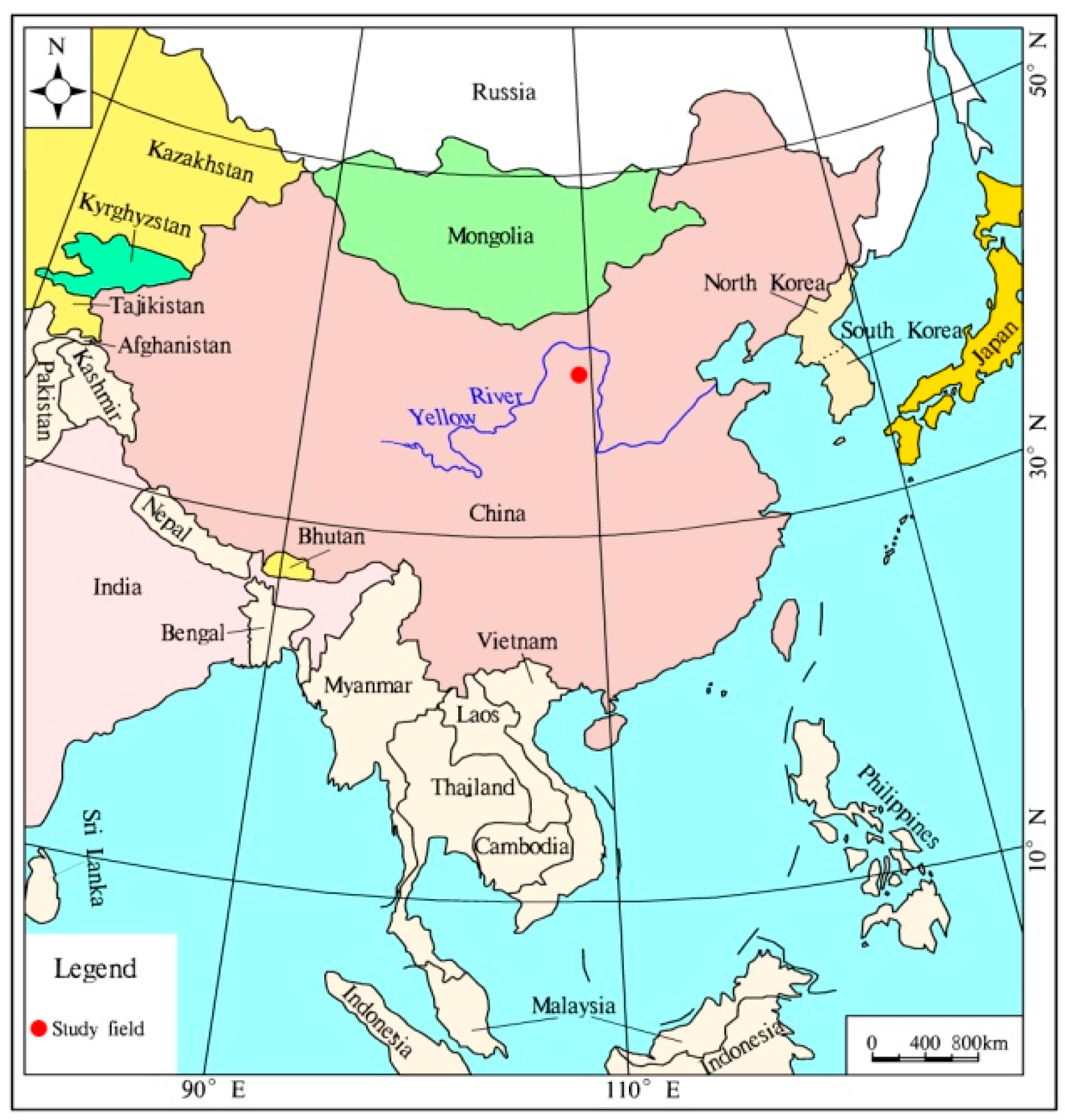
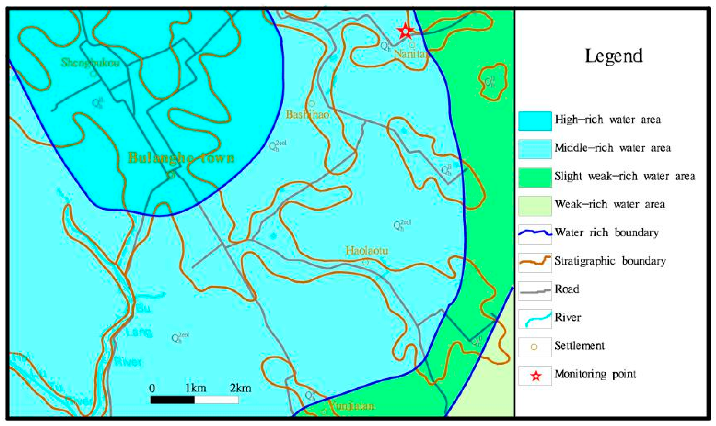
The study was conducted in the southern margin of the Mu Us Sandy Land, Bulanghe Township, Yulin City, China (Figure 1). It is located in the water shed of Bu Lang River, a tributary of Hai Liu Tu River. The surface layer in this area is aeolian sand, underlying sandstone or mudstone, and the main aquifer is the Quaternary Lake sediments’ pore aquifer ($Q_h^{1l}$), a middle-rich water area (Figure 2). Soils are fine-textured sand without clay, according to the grain size composition experiment at the test site (

Table 1. Soil texture information of different layers.

Depth	Sand	Silt	Bulk Density
(cm)	(%)	(%)	(g/cm3)
0–20	96.0	4.0	1.606
20–80	98.4	1.6	1.634
80–150	99.0	1.0	1.701

). The depth of phreatic water is about 1.1–1.4 m. Altitude is 1250–1280 m and the average annual temperature is 8.1 °C. It experiences a typical semi-arid climate: precipitation is mainly concentrated from June to September, with an average annual precipitation of 340 mm and an average annual potential evaporation of 2180 mm from 1957–2007 [38].

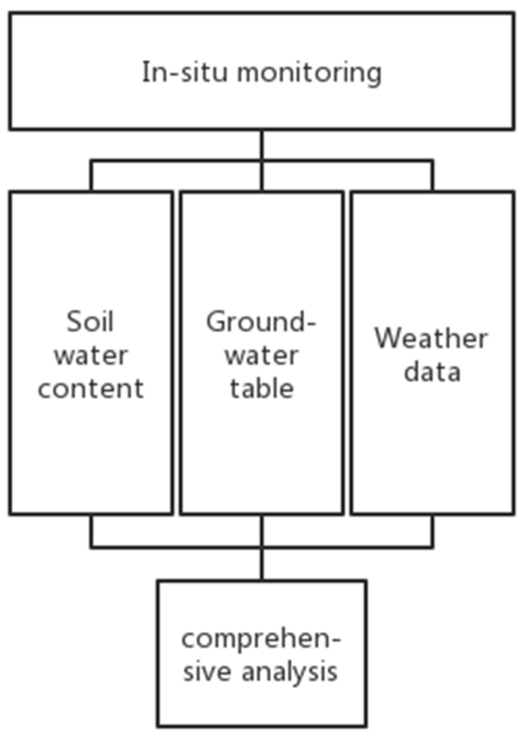
The test site is located at the observation base for groundwater and ecology of the Chinese Land and Resources Ministry in Yulin, Shaanxi Province. A gently-fixed dune covered by no vegetation on the site was selected to monitor water content, temperature, matrix potential, and water table. We obtained precipitation, net radiation, and other weather data on site. Water content and temperature in the vadose zone were monitored by Temperature and Moisture with 5-point calibration program(5TM) sensors (Meter Group, Inc., Pullman, USA) buried in the ground at 5, 10, 30, 60, and 90 cm depths. Meteorological data were automatically monitored by the 05130-5RM Yong system (Compbell, Inc., USA) within the test site. The water table was automatically monitored by the MiniDiver and the probe was buried 160 cm below the surface. Data collection intervals were 1 h for the water table and 10 min for the weather data. The infiltration and groundwater recharge law were primarily analyzed according to the in situ test data in the study area (Figure 3).

2.2. Field Data Analysis

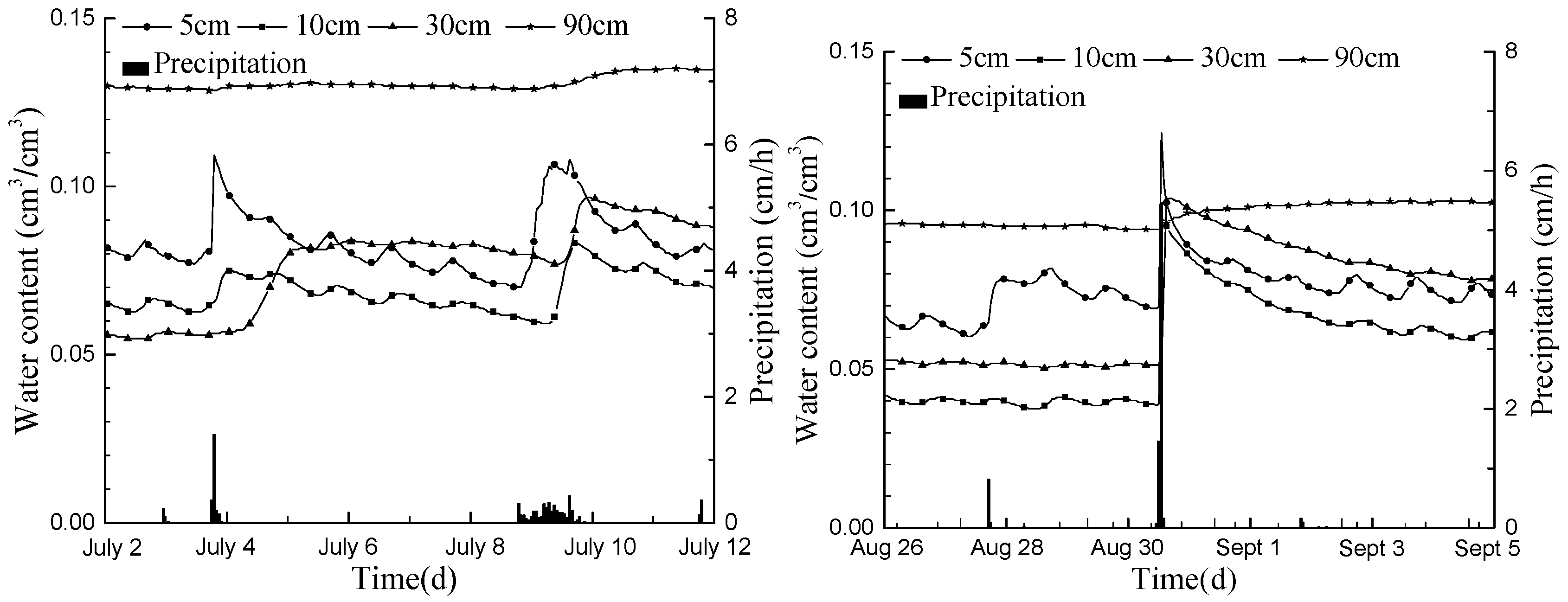
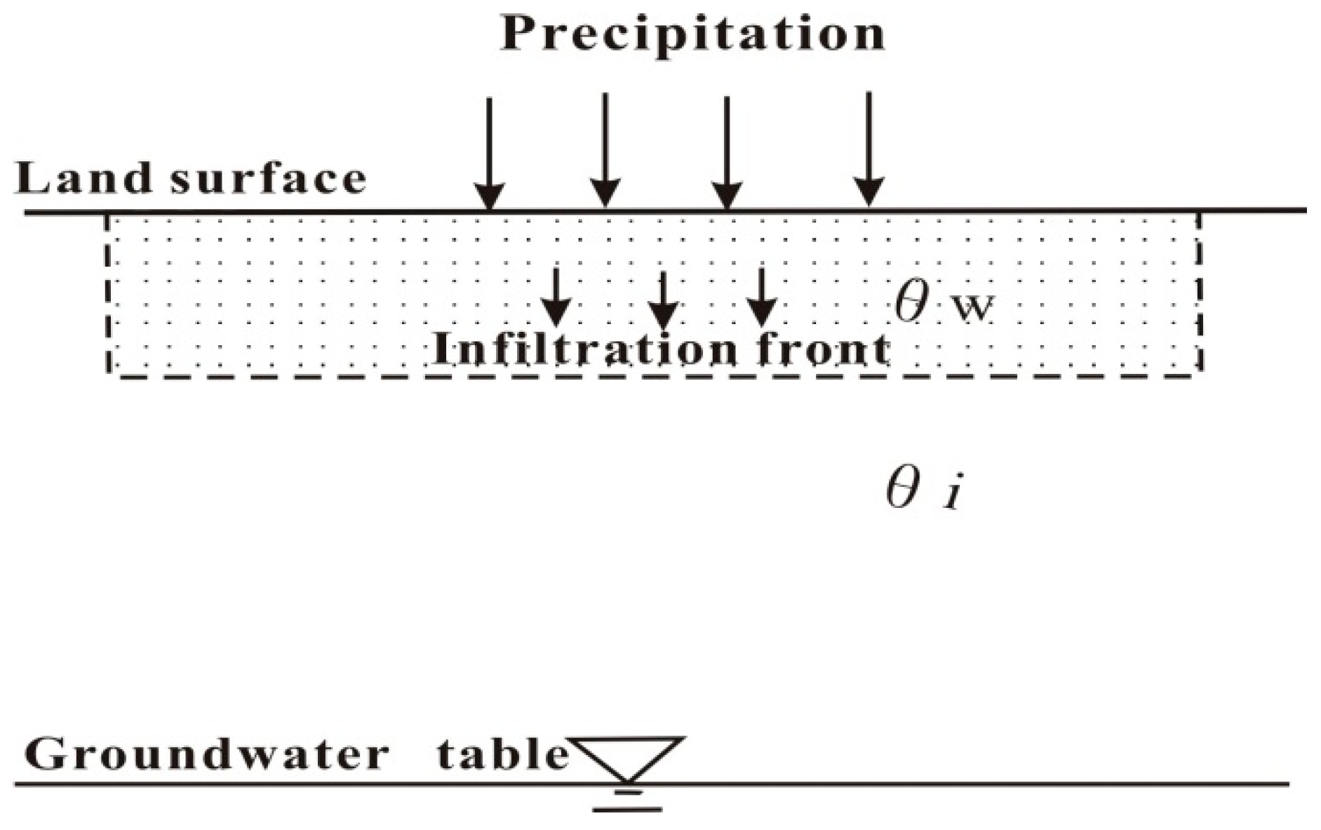
Over 2500 h of observed data of water content and water table (from 2 July to 15 October 2014) were analyzed in this paper. The shallower the depth of the vadose zone was, the quicker the water content increased after precipitation. The greater precipitation was, the deeper the response depth of the vadose zone. For example (Figure 4), on 27 August 2014, the precipitation was 0.82 cm (small rain). There was a response at a 5 cm depth, with no obvious change at greater depths. Precipitation on 30 August was 7.1 cm (rainstorm), the water content at all depths of the vadose zone increased significantly. The infiltration process is illustrated in Figure 5, where ${\theta }_w$ is the water content upon the infiltration front, often near the field capacity, ${\theta }_i$ is the initial water content in the vadose zone, the dotted lines are the infiltration fronts. During our study period, infiltration was totally non-ponding, as the rain intensity was usually less than the infiltrability. The unsaturated flow moved downwards with time, driven by gravity and capillary force. Water content was still ${\theta }_i$ below the infiltration front while water content increased heavily above that front. The infiltration would keep moving and may eventually reach the water table if the water supply at surface was sufficient.

With the increase of depths of the vadose zone, there was a significant time lag on the response of water content. The response lag time of water content in the vadose zone refers to the time interval between precipitation and consequent water content rising. On 8 July, the lag time was 5 h at 10 cm, 9 h at 30 cm, and 17 h at 90 cm, (Figure 4). The infiltration rates appeared to be higher at deeper vadose zones. Unlike ponded infiltration, precipitation infiltration, depending on hydraulic conductivity and water potential gradient, are mainly unsaturated flow, its conductivity is always lower than saturated conductivity K_S. Though the higher potential gradient in the shallow soil due to the quite low-water content, infiltration rates in the deep soil, where water content was higher than the shallow part, was higher due to the relative high conductivity. The response depths of major precipitations are shown in Table 5 from March to October 2014. Since the maximum monitoring depth was 90 cm, depths which were more than 90 cm are expressed by 90+. All the response depths of storm rains were more than 90 cm, while all that of small rains were less than 10 cm.

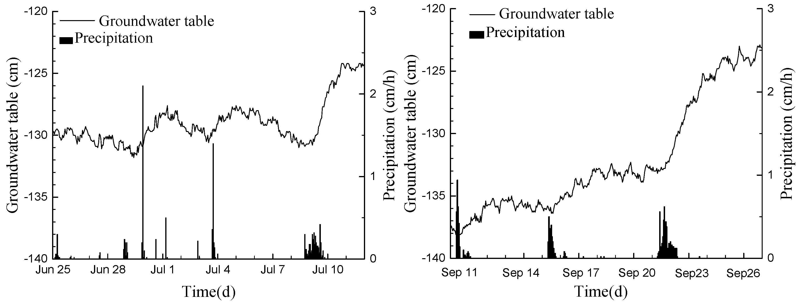
Water tables did not rise until infiltration was eventually reached. The recharge lag time from a recent precipitation (2.24 cm) event occurring on 29 June was 4 h. From the precipitation event (2.12 cm) on 3 July, it was 5 h (Figure 6). From the beginning of the precipitation recharge, the recharge process can be divided into two stages. The first stage involving the rapid rise of the water table, is assumed to be predominately unsaturated gravitational vertical flow, when the recharge increases sharply, and the recharge rates are quite high. The second stage is the slowly rising stage of the water table, when the recharge increases slowly and the recharge rates are quite small, even close to zero, which may result, in part, due to the horizontal flow. For example, the water table rose by 1.1 cm in 5 h after the precipitation event on 3 July, and only increased by 0.4 cm during the next 15 h. Also, note the water table responses to precipitation events occurred before notable water content changes in the vadose zone (Figure 4), suggesting mostly sub-saturated flow. This pre-saturated preferential flow may affect the differences among infiltration lag times across different depths in the vadose zone.

2.3. Numerical Model Setup

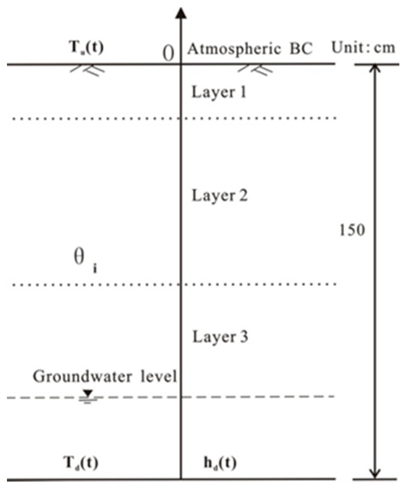
To better understand the lag effects in precipitation infiltration and remove the influence of preferential flow on infiltration and to determine recharge lag time accurately, a numerical model water, vapor, and heat in the variably-saturated zone based on Hydrus-1D software was established in this report. The soil surface was selected as the origin of the coordinates and the upward direction was positive. The conceptual model of hydrogeology is shown in Figure 7. Soil surface is the upper boundary of the model. On this boundary, precipitation infiltrates and soil water evaporate; heat exchange takes place between the soil and the atmosphere. The sand modeled column extended to a depth of 150 cm (about 30 cm under the water table). The total column contained three layers based on particle analysis and bulk density, 0–20 cm was the first layer, 20–80 cm the second one, and 80–150 cm the third. The pressure head at the lower boundary varies with the change of water table, ignoring horizontal diffusion, which can be regarded as a one-dimensional vertical transient flow model of a “variably saturated zone”. In the figure, $T_d\left(t\right)$ is the temperature of lower boundary, $T_u\left(t\right)$ for the upper boundary, $h_d\left(t\right)$ is the pressure head at the lower boundary; ${\theta }_i$ is the profile water content distribution at initial time. The media can be classified into three layers according to the particle analysis and the bulk density, 0–20 cm is the first layer, 20–80 cm is the second one, and 80–150 cm the third one.

The mathematical model is provided as Equation (1).

$$\{\begin{array}{l}\frac{\partial \theta }{\partial t}=\frac{\partial }{\partial z}\left[K_{Th}\frac{\partial h}{\partial z}+K_{Lh}+K_{TT}\frac{\partial T}{\partial z}\right]\\ C_p\left(\theta \right)\frac{\partial T}{\partial t}+L_0\frac{\partial {\theta }_V}{\partial t}=\frac{\partial }{\partial z}\left[\lambda \left(\theta \right)\frac{\partial T}{\partial z}\right]-C_w\frac{\partial q_{L}T}{\partial z}-L_0\frac{\partial q_V}{\partial z}-C_V\frac{\partial q_{V}T}{\partial z}\\ T_u=T_{ui}{T}_d=T_{di}t=0\\ \theta ={\theta }_{i}t=0z\le 0\\ T_d=T_d\left(t\right)T_u=T_u\left(t\right)t>0\\ h_d=h_d\left(t\right)t\ge 0\end{array}$$

(1)

In Equation (1), $K_{Th}$ is the isothermal total hydraulic conductivity (L/T), $K_{Th}=K_{Lh}+K_{Vh},\mathrm{where}{K}_{Lh}$ is the isothermal liquid water hydraulic conductivity (L/T); $K_{Vh}$ is the isothermal vapor hydraulic conductivity (L/T); $K_{TT}$ is the total water hydraulic conductivity driven by temperature gradient (L²/T(K), $K_{TT}=K_{LT}+K_{VT},K_{LT}$ is the thermal liquid water hydraulic conductivity (L/T); $K_{VT}$ is the thermal vapor hydraulic conductivity (L²/TK);$C_p\left(\theta \right)$ is the soil heat capacity (ML/T²K); ${\theta }_V$ is the volume content of water vapor in the soil (L³/L³); $\lambda \left(\theta \right)$ is the thermal conductivity (ML/T³·K); $T_u\left(t\right)$ is the time varied temperature on the upper boundary (K), $T_d\left(t\right)$ is the time-varied temperature on the lower boundary(K), $\theta$ is the volumetric soil water content (L³/L³), $h_d\left(t\right)$ is the time varied pressure head on the lower boundary (L). $T_{ui}$ and $T_{ui}$ are the initial temperature at the upper and lower boundary.

The atmospheric boundary was used as the upper boundary, while a variable pressure head condition was used as the lower boundary. The heat boundary conditions were the temperatures at the upper and lower boundaries. The initial temperature condition was the temperature measurement at the initial time. The initial water content condition was the water content distribution in equilibrium with the initial water table calculated by Hydrus-1D. We used a constant head condition at the bottom boundary at the numerical model and set it equal to the pressure head at initial time, namely, the head at the bottom boundary was always equal to the initial head and the water content distribution was obtained after more than three months of calculation, ensuring there was no influence of precedent rainfall.

Van Genuchten’s equation was selected as the hydraulic model, as shown in Equations (1) and (2) [39].

$$\theta \left(h\right)=\{\begin{array}{c}{\theta }_r+\frac{{\theta }_s-{\theta }_r}{{\left[1+{\left|\alpha h\right|}^n\right]}^m}h<0\\ {\theta }_{s}h\ge 0\end{array}$$

(2)

$$K\left(h\right)=K_s{S}_e^l{\left[1-{\left(1-S_e^{\raisebox{1ex}{$1$}\!\left/ \!\raisebox{-1ex}{$m$}\right.}\right)}^m\right]}^2$$

(3)

where:

m = 1 − 1/n

(4)

${\theta }_r$ is the residual soil water content. ${\theta }_s$ is the saturated water content. α and n are parameters in the soil water retention function. $K_s$ is the saturated hydraulic conductivity. h is the pressure head. l is the pore connectivity parameter for soil.$S_e$ is the effective saturation:

$$S_e=\frac{\theta -{\theta }_r}{{\theta }_s-{\theta }_r}$$

(5)

And the hysteresis effect of water retention curve was considered. Additional parameters ${\theta }^m$, ${\theta }_s^w$, ${\alpha }^w$, are used to describe the wetting curve in the soil water retention function when considering hysteresis. We did not consider the hysteresis effect of hydraulic conductivity in this case. So saturated hydraulic conductivity in wetting curve $K_s^w$ equals to $K_s$.

2.4. Model Parameters

The initial soil hydraulic parameters were obtained by a neural network predictions module in Hydrus-1D based on particle analysis and bulk density. After that, parameters were obtained by model calibration.

In calibration and following validation, the simulation’s performance compared with the observed data was evaluated by the relative average error (AVRE) and the correlation coefficient (R).

$$AVRE={{\displaystyle \sum }}^{}\left(V{C}_I/V{O}_I\right)/n$$

(6)

$$R=\frac{{{\displaystyle \sum }}_{i=1}^n\left(v{c}_i-\overline{vc}\right)\left(v{o}_i-\overline{vo}\right)}{\sqrt{{{\displaystyle \sum }}_{i=1}^n{\left(v{c}_i-\overline{vc}\right)}^2·{{\displaystyle \sum }}_{i=1}^n{\left(v{o}_i-\overline{vo}\right)}^2}}$$

(7)

In Equations (2) and (3), $V{C}_i$ is the simulated value, $V{O}_i$ is the observed value, $n$ is the total number of data. $\overline{vo}$ is the average value of observed data, and $\overline{vc}$ is the average of simulated data.

Basic hydraulic and heat parameters were obtained after calibration, shown in

Table 2. Hydraulic parameters obtained by the model after calibration.

Layer	${\mathit{\theta }}_{\mathit{r}}$	${\mathit{\theta }}_{\mathit{s}}$	$\mathit{\alpha }$	n	${\mathit{K}}_{\mathit{s}}$	l	${\mathit{\theta }}^{\mathit{m}}$	${\mathit{\theta }}_{\mathit{s}}^{\mathit{w}}$	${\mathit{\alpha }}^{\mathit{w}}$	${\mathit{K}}_{\mathit{s}}^{\mathit{w}}$
	(cm3/cm3)		(cm−1)		(cm/h)		(cm3/cm3)		(cm−1)	(cm/h)
1st	0.032	0.34	0.062	2.1	23	0.5	0.344	0.32	0.06	23
2nd	0.032	0.34	0.060	2.2	23	0.5	0.344	0.32	0.06	23
3rd	0.032	0.34	0.074	2.0	23	0.5	0.344	0.32	0.07	23

and

Table 3. Heat parameters obtained by the model after calibration.

Layer	Solid	Disp	b1	b2	b3	Cn	Cw
		(cm)	(W·cm−3·k−1)			(J·cm−3·k−1)
Layers 1–3	0.656	5	1.28 × 1010	−5.05 × 1012	1.51 × 1013	5.50 × 1010	5.24 × 1011

$b1$, b2, b3 are coefficients in the expression for the thermal conductivity $\lambda \left(\theta \right)$. C_n is the volumetric heat capacity of the solid phase. C_w is the volumetric heat capacity of the water phase. Disp is the longitudinal thermal dispersity. Solid is the volume fraction of the solid phase.

. Total AVRE of water content is equal to 1.178 in the calibration period (00:00, 2 July to 00:00, 15 July) and to 1.114 in validation period (00:00 on 15 July to 00:00 on 13 August). Additional Supplementary Materials may be found with the online version of this article.

3. Results and Discussion

3.1. Precipitation Infiltration Process

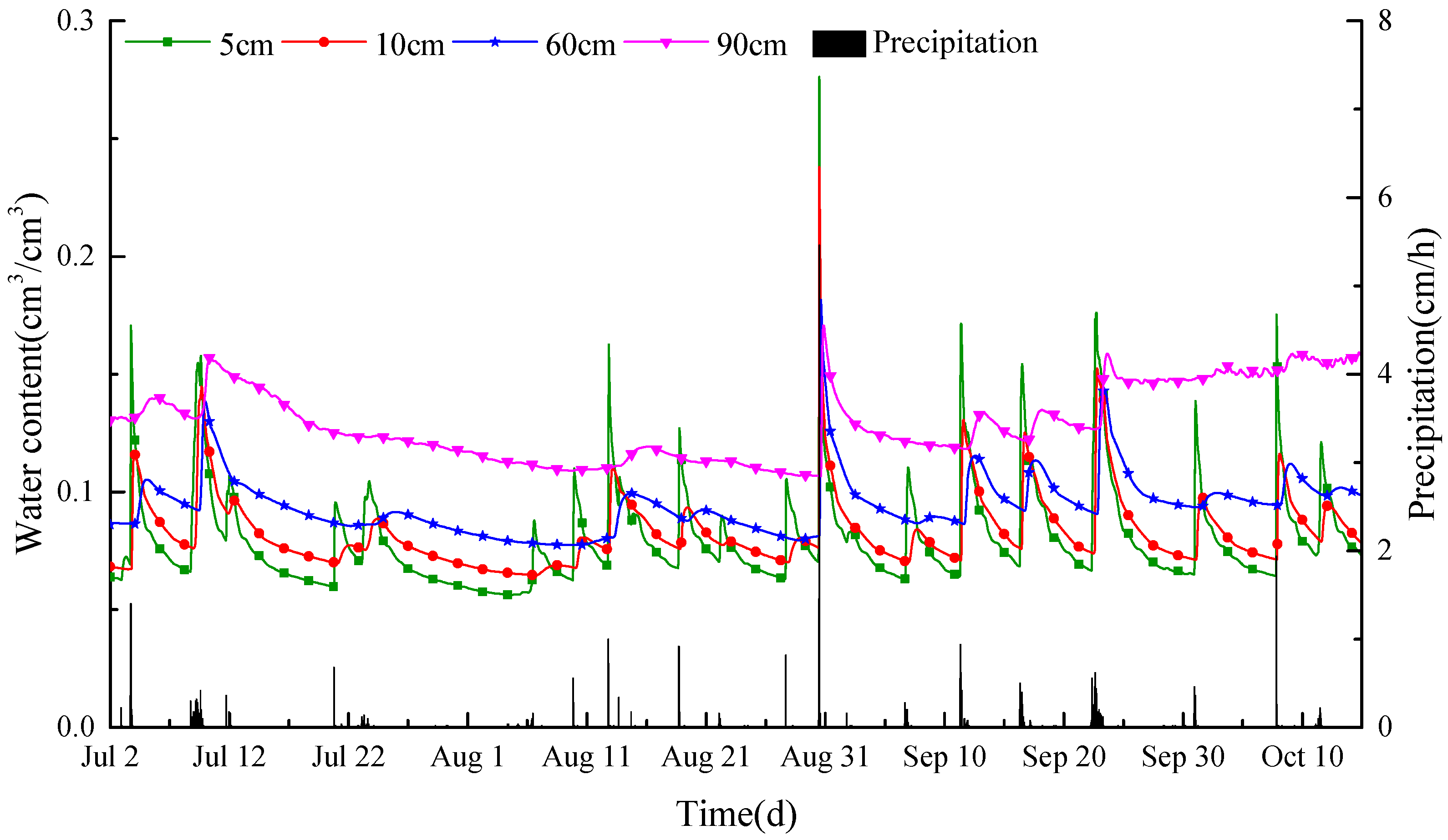
Data from 2544 h were selected for infiltration analysis during the precipitation concentrated period (00:00 on 2 July to 23:00 on 15 October 2014). The groundwater depths in this period were about 120–140 cm. The precipitation and simulated soil water content time series are shown in Figure 8. Water content at 5, 10, 60, and 90-cm depths all increased after precipitation, and that in the upper part responded intensively. However, there was a significant time lag between response of soil water content and the precipitation events in both the unsaturated vadose zone and saturated water table. The greater the depth of the vadose zone, the longer the lag time.

In order to study the influence of different types of rainfall on water content in the vadose zone and groundwater, this paper classified rainfall according to

Table 4. Rain type classification.

Range	Rain in 1 h (mm)	Rain in 12 h (mm)	Rain in 24 h (mm)
Small rain	≤2.5	≤5	<10
Middle rain	2.5–8	5–15	10–24.9
Heavy rain	8–16	15–30	25.0–49.9
Storm rain	≥16	≥30	≥50

[40].

This table helps to classify all rain events which happened during the study period. Note that rains that reached two or three different rain types were classified as the highest type.

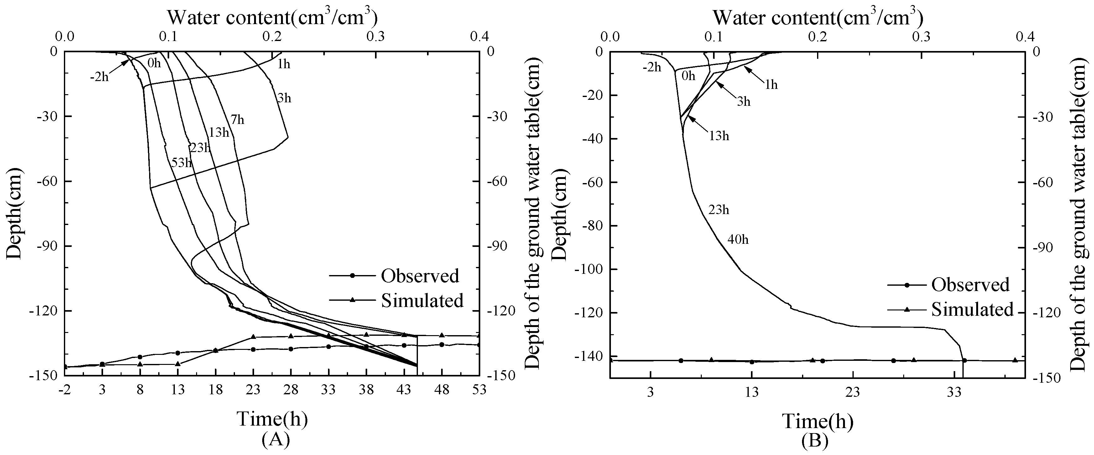
Figure 9A shows a storm rain (total amount 71.6 mm), where −2 h is the distribution of water content at 2 h before rainfall, 53 h was the distribution at 53 h after rainfall. Water content on the surface immediately rose and reached the maximum value at 2 h after rainfall; but gradually decreased due to evaporation and infiltration. Water content in the deeper layers increased continuously but with a time lag.

A recharge front was defined as the interface between the rising zone and the unchanged zone of water content, above which water content rose and below which water content remain unchanged. During the infiltration process, the recharge front moved to 15 cm in 1 h, 65 cm in 3 h, and 95 cm in 7 h. The maximum moving rate of the recharge front appeared in 0–3 h, corresponding to the maximum rainfall intensity (2 h after the start of precipitation). The deep vadose zone (near the water table) was within the capillary saturated zone, so water content variation was quite small. With the increase of water content in the entire vadose zone, infiltration reached the water table. Figure 9A shows that the observed time of water table rising (3 h) was significantly earlier than the model result (13 h), and the amplitude was also smaller. Water content in the entire vadose zone approximately returned to the pre-rain distribution after 53 h, indicating the influence of this rain tended to disappear.

Figure 9B shows a middle rain (total 8.8 mm). Water content of the upper layer also responded sensitively, but the response depth of water content was smaller than the former above. Recharge front reached only 35 cm; below which water content did not change during the entire infiltration process. Also, the water table did not respond after this rainfall.

3.2. Precipitation Infiltration Recharge

Precipitation in this area is mainly concentrated in the wet season (June–September), accounting for 80–90% of the annual precipitation. A total 5211 h of a free-freezing period from March to October was selected as a research period. The groundwater recharge was calculated by accumulative water flux near the water table during a recharge period. Water table depth varied from about 1.2 m to 1.4 m throughout a hydrological year.

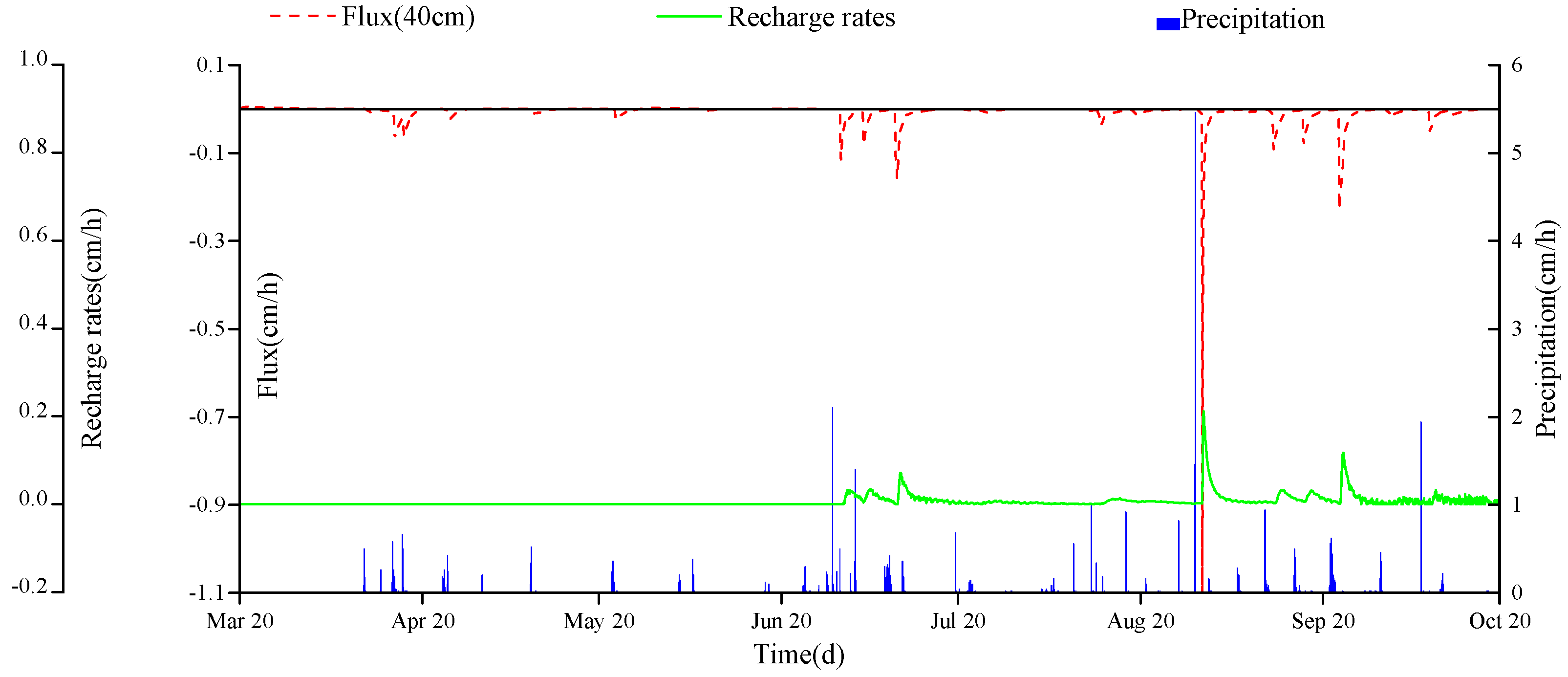
The solid-green line in Figure 10 is the groundwater recharge rate (GRR). The red-dotted line is the water flux at the depth of 40 cm (F) in the vadose zone; a negative value indicates the downward direction. The positive F was quite small in the research period, indicating that the water flux at this depth was very weak. Before June, GRR remained 0 though the total precipitation was 121 mm. The groundwater recharge was mainly concentrated in the period from July to September. In this period, the total recharge accounted for over 90% of the annual recharge, reaching 268 mm. The peaks of F were consistent with the peaks of precipitation, but with a slight lag about 5–10 h. The GRR, smaller than F, also lagged behind F. The difference between GRR and F became greater after a storm rain than a heavy rain. For example, after the storm rain (total 71.6 mm) on 29 August, the peak value of F was −1.5 cm/h, and the peak value of GRR was only 0.2 cm/h. Due to the obvious wet and dry interface at the upper layer during infiltration, leading to a larger hydraulic gradient, the flux of the upper layer was quite higher than GRR.

Twelve different precipitations were selected in 2014 and the precipitation recharge coefficients (α) for each precipitation were calculated and compared with the values based on the observation water table fluctuations. The results are shown in

Table 5. Recharge coefficients of precipitation obtained by the model and field data.

Recharge Parameters		Small Rain			Middle Rain			Heavy Rain			Storm Rain
		1	2	3	1	2	3	1	2	3	1	2	3
Precipitation (mm)		8	2.4	4	8.8	17.4	11.2	21.2	41.4	30.6	71.6	54.6	22.4
Initial depth (cm)		134	130	144	142	142	143	130	131	138	146	133	122
Response depth (monitoring data) (cm)		10	5	5	30	90+	30	60	90+	90+	90+	90+	90+
α	Field measured	-	-	-	-	0.17	-	0.36	0.48	0.28	0.54	0.61	0.21
	Modeled	-	-	-	-	0.47	-	0.56	0.42	0.35	0.64	0.67	0.16

. There was no recharge after small precipitation events. “Calculated” in this table refers to an α value based on the observed water table fluctuations and “Simulated” refers to α value calculated by the model.

According to Table 5, heavy rain and storm rain during the study period all effectively recharged groundwater. In general, the precipitation recharge coefficient (α) increased with the increase of precipitation. For example, α of the first storm rain was larger than the third storm rain, and the second storm rain was larger than the third heavy rain. It seems that the storm rain events, which had higher α than other rain types, were more favorable to groundwater recharge in this area, similar to the results in the upper Nile River zone [41,42]. This can be explained by the relationship between evaporation and precipitation. The total evaporation (TE) from the end of the first storm rain to the end of groundwater recharge (total 72 h) was 0.65 cm. Total evaporation was 0.43 cm from the end of the third storm rain to the end of groundwater recharge (total 42 h). Evaporation intensity was quite close after the two precipitations; then TE was mainly determined by the evaporation time length. Additionally, the water stored per unit area in the 0–50 cm depth of the vadose zone was close, 3.75 and 3.55 cm³/cm², respectively. Therefore, when the recharge time durations after rain were close, the larger the precipitation there was, the smaller the proportion of TE and water deficit in the vadose zone to the precipitation was, and the larger α was (for detailed information, refer to equations for calculating recharge in

Table 6. Simulated water balance components from March to December 2014 (in mm and % of precipitation).

Recharge Parameters	Amount (mm)	%
Precipitation (P)	568	100
Actual Evaporation (E)	217.3	38.3
Runoff (RO)	0	0
Net infiltration (I)	350.7	61.7
Transpiration (T)	0	0
Change in storage in the vadose zone (CW)	+80.5	14.2
Recharge (R)	268.8	47.3
(R = P − E − RO − T – CW + ER)
Simulated mass balance Error (ER)	−1.4	−0.2

, R = P-E-RO-T-CW+ER, where RO and T equal to 0). There is an exception for α: the α value of the second storm was larger than that of the first storm. This can be explained by the different duration of these two rainfalls, 26 and 4 h. Evaporation was quite weak during rainfall, meaning that the second storm experienced a weak evaporation period in the early recharge process.

α values obtained from this model were generally larger than those measured field data. The reason is that the model used a one-dimensional flow calculation, ignoring horizontal runoff, resulting in larger values of the recharge coefficients. The difference between the calculated and the observed values for the second middle rain was relatively large; α were 0.47 and 0.17, respectively. This was due to the relatively small amount of rainfall (17.4 mm) and weak response of the water table; then the water table fluctuation may be obscured by natural water table noise, resulting in a small increase in the observed water table, similar to the results of Carling [43].

Table 6 summarizes the balance components during March to December 2014. The vegetation transpiration was 0 for the bare soil. We used water storage of the entire profile minus that of the saturation zone to calculate water storage in the vadose zone. Net infiltration was calculated by subtracting actual evaporation from precipitation. According to the water balance, the total recharge in 2014 was 268.8 mm. Note that the total recharge obtained by accumulating the fluxes near the water table was 294 mm. This error was mainly caused by the difference in the flux between the model observation point location and the actual water table during the water table fluctuation.

3.3. Invalid Precipitation

A period was selected in which small rain occurred and the rainfall conditions changed. Setting the precipitation to 0.4, 0.6, 0.8, 0.9, and 1 mm in 1 h, respectively, it was found that precipitations of 0.9 and 1 mm can change water content of the surface, indicating the invalid precipitation on the surface was 0.8–0.9 mm in 1 h.

Another two periods were selected in which water depths were about 120 and 140 cm. Water distribution was calculated by a Hydrus model. The upper boundary condition was zero flux boundary and the bottom boundary condition was a constant head in this model. We used this water distribution as the initial condition in invalid precipitation prediction to eliminate the effect of precedent moisture. By changing the rainfall conditions, it was found that the invalid precipitation at the water table was 11.25–11.75 mm in 1 h when the depth was 120 cm, and was 15–15.5 mm when the depth was about 140 cm. The precipitation less than invalid precipitation cannot recharge groundwater, and can only supply the water deficit in the vadose zone. All these invalid precipitations were calculated based on summer data, due to abundant rainfall.

The invalid precipitation in this paper was calculated from the total precipitation within 1 h. Note that the total precipitation of 24 mm was larger than the invalid precipitation on April 17 (groundwater depth was 143 cm), but there was no recharge as this precipitation lasted for 17 h and the maximal precipitation intensity (14 mm/h) was smaller than the invalid precipitation obtained by this paper. Furthermore, quite scarce precipitation in the spring, which means a large water deficit in the vadose zone, dry sand layer in some areas, all leads to a larger invalid precipitation for groundwater recharge than this paper.

3.4. The Response Lag Time of Infiltration Recharge

3.4.1. Recharge Lag in Vadose Zone

We determined lag time by simulated water content time series in this paper. After different precipitations, the response lag time of water content at 10, 30, 60, and 90 cm in the vadose zone are shown in

Table 7. Infiltration lag times at different depths after precipitation.

Intensity Lag Time (h)		Small Rain			Middle Rain			Heavy Rain			Storm Rain
		1	2	3	1	2	3	1	2	3	1	2	3
Rain (mm)		8	2.4	4	8.8	17.4	11.2	21.2	41.4	30.6	71.6	54.6	22.4
Soil depth	10 cm	3	-	-	1	1	<1	1	2	1	<1	1	<1
	30 cm	-	-	-	11	10	12	4	9	4	2	5	3
	60 cm	-	-	-	-	16	-	13	16	10	3	12	8
	90 cm	-	-	-	-	25	-	19	18	18	6	18	16
ACR (mm)	36 h	0.8	2.2	0.4	5.6	10	9.2	6	3	5.6	0.8	7.2	19.4
	48 h	1.4	2.2	0.4	5.6	10	9.2	6	3	5.6	0.8	7.2	19.4
	96 h	8.4	2.2	11.6	11.4	18.8	9.4	6	3	5.6	9.2	7.6	19.4
	120 h	8.4	2.2	11.6	12.2	18.8	11.2	6	6.6	15.2	9.2	7.8	19.4
	144 h	8.4	2.2	11.6	13	19	32.2	6	26.6	15.2	9.4	23.6	19.4

NOTE: The “ACR” refers to the accumulative rainfall before this precipitation event.

. The “ACR” refers to the accumulative rainfall before this precipitation event.

As shown in Table 7, the maximum effect depth of small rain was only 10 cm. After small rain, water evaporated rapidly and there was no obvious change of water content in the vadose zone. Under the same precipitation, the greater the depth of the vadose zone, the longer the response lag time of water content. The lag time at 10 cm was usually shorter than 2 h while it was usually 16–25 h at 90 cm. The response lag time of water content was smaller in wet periods than in dry periods, similar to Lee’s results [44]. This actually indicated the effect of the cumulative precipitation during the previous period. The larger the cumulative precipitation in the previous period was, the higher the initial water content in the profile was; thus, shortening the infiltration time and reducing the lag time of water content. For example, the total precipitation of the second storm rain (54.6 mm) was much greater than the third storm rain (22.4 mm), but the cumulative precipitation in 36 h before the former was only 7.2 mm, much less than the accumulative precipitation in 36 h before the latter (19.4 mm). That led to a greater vadose zone deficit than the latter, so the water content response lag time of each depth in the vadose zone was longer than the latter. Note that the accumulative precipitation in 144 h before the first heavy rain and the second heavy rain differed greatly, but there was no significant difference in the response lag time at all depths. It suggested that the cumulative precipitation can only affected on latter recharge within 144 h.

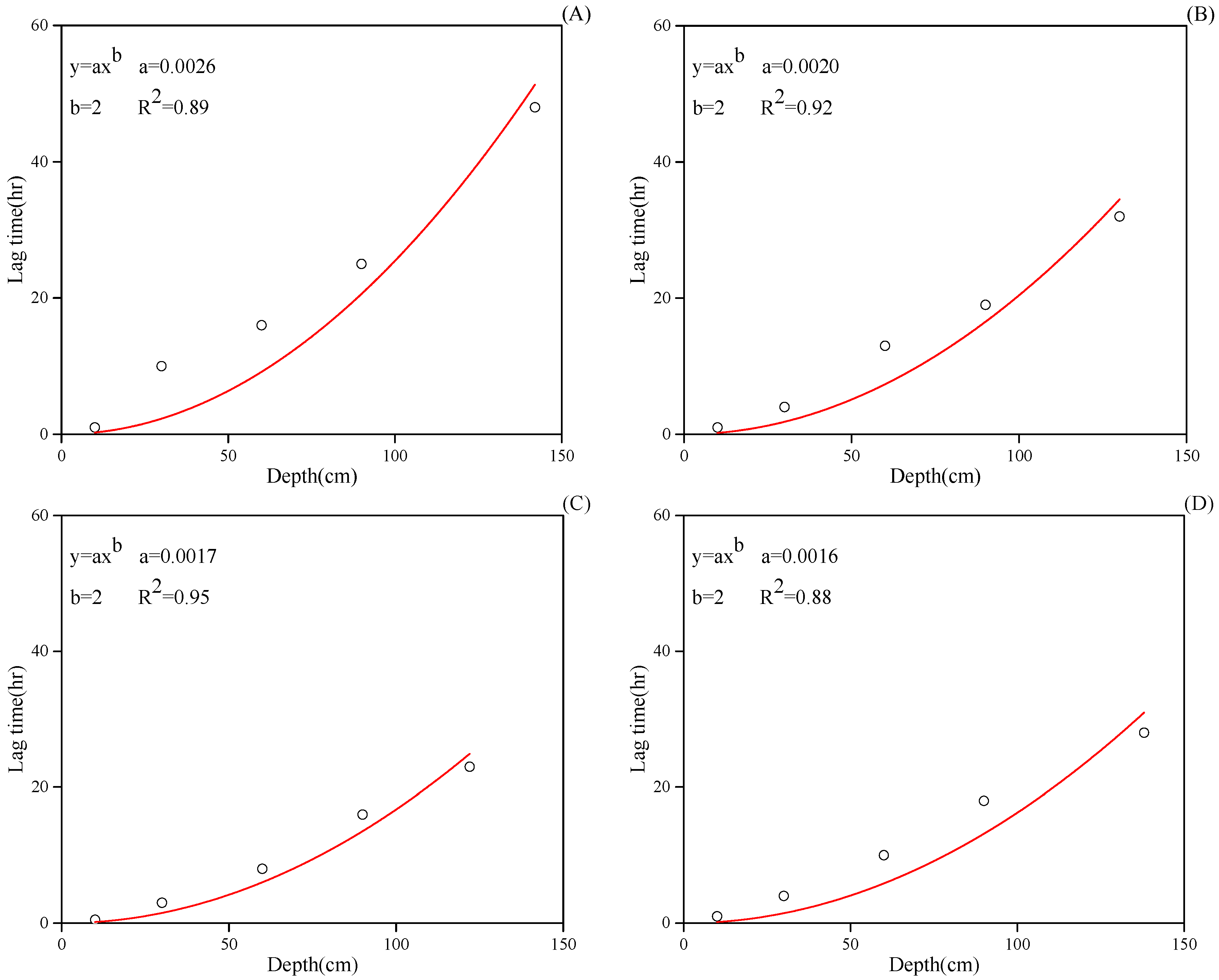
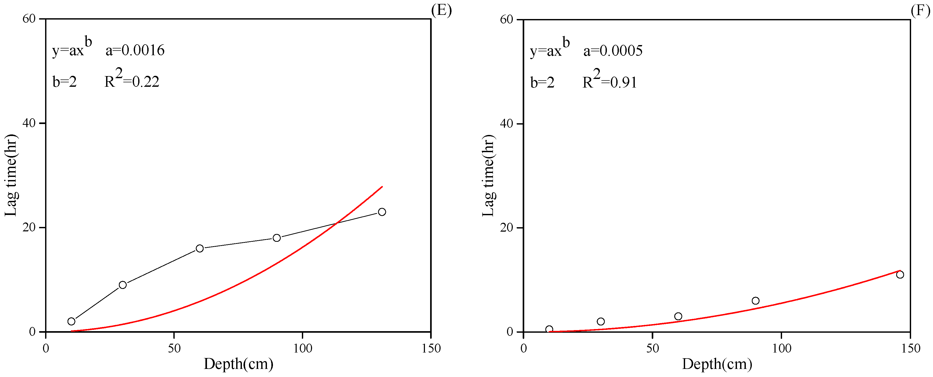
The plots of lag time of water content in the vadose zone versus soil depths (Figure 11) show that the response lag times of water content in the vadose zone increased with the soil depth. Correlation analyses were conducted between lag time and soil depth. All the lag times were proportional to the square of depths only remaining with some deviation following rains of 54.6 mm (E). The plot (E) shows that lag time increased very slowly as soil depths go deeper, opposite to the other plots. The obvious change in slope (about lag time at 17 h) in the data curves in (E) suggests that the moving speed of infiltration front was greater after 17 h. This may be caused by the different rain patterns between (E) and others. The total rainfall of (E) was 41.4 mm but lasted more than 30 h, the soil would absorb the water and acquire a wetness for which the conductivity was equal to the water supply rates after this long time. So, the infiltration rates are greater as the rainfall intensity become greater after 17 h, see Figure 8.

Figure 11 shows relationships between the response lag times of water content in the vadose zone and the soil depths. Correlation analyses were conducted between lag time and soil depth. All the lag times were almost significantly proportional to the square of depths, indicating that infiltration was dominated by matrix flow at this monitoring point. But some deviation following rains of 54.6 mm (E) remains. The plot (E) shows that lag time increased very slowly as soil depths go deeper, opposite to the other plots. The obvious change in slope (about lag time at 17 h) on the data curve in (E) suggests that the moving speed of the infiltration front was greater after 17 h. This may be caused by the different rain patterns between (E) and the others. The total rainfall of (E) was 41.4 mm but lasted more than 30 h, the soil would absorb the water and acquire a wetness for which the conductivity was equal to the water supply rates after this long time. So, the infiltration rates were greater as the rainfall intensity become greater after 17 h, see Figure 8.

Precipitation of 8.8 mm can result in a response at a 30-cm depth in the vadose zone, while the results obtained by Xinping Liu was 11.8 mm [45], mainly because that the groundwater depth (13–15 m) in Liu’s study area was much deeper than in our study area (1.1–1.4 m).

At the same depth, the greater the precipitation was, the shorter the response time lag of water content in the vadose zone was. For middle rain, the lag time was 1 h at 10 cm, 16 h at 60 cm, and 1–2 h, 13–16 h for heavy rain, and less than 1 h, 3–12 h for storm rain, respectively. The calculation results were similar with field studies in this area [34]. Nevertheless, there remains some disagreement between the modeled and field results at 10 cm when the precipitation was small. This error might result from the restriction of the minimum time interval of the model input conditions, 1 h, which may be longer than the lag time at 10 cm. This results in an inaccuracy of the model input data, so the model prediction accuracy can be significantly improved by improving the precipitation data input accuracy [46].

3.4.2. Recharge Lag of Groundwater

Under different precipitation types and conditions, water table response was quite different. The time interval between the initial response time of water content to the ceases time of water content rising is regarded as the duration of recharge.

Table 8. Groundwater recharge lag times and recharge durations after precipitation.

	Small Rain			Middle Rain			Heavy Rain			Storm Rain
	1	2	3	1	2	3	1	2	3	1	2	3
Rain (mm)	8	2.4	4	8.8	17.4	11.2	21.2	41.4	30.6	71.6	54.6	22.4
Initial depth (cm)	134	130	144	142	142	143	130	131	138	146	133	122
Rain duration (h)	16	3	6	4	5	2	5	27	18	4	26	5
Lag time (sim) (h)	-	-	-	-	48	-	32	23	28	11	20	23
Lag time (obs) (h)	-	-	-	-	7	-	7	11	8	3	6	4
Recharge duration time (h)	-	-	-	-	98	-	102	155	80	65	95	24

shows the lag time of water table response and the recharge duration of different types of precipitation. Lag time (sim) and Lag time (obs) mean modeled and observed values, respectively. The recharge duration and recharge lag time were determined by simulated water flux time-series at water table.

It can be seen from Table 8 that small rain cannot recharge groundwater. Despite the influence of precipitation duration, the amount of precipitation also effects recharge duration. The smaller the precipitation was, the longer recharge duration. Comparing the second heavy rain (total duration 27 h and total precipitation 41.4 mm) with the second storm rain (total duration 26 h and total precipitation 54.6 mm), the former recharge duration was 155 h and the latter was 95 h. Also, recharge duration of the third storm (total 22.4 mm, max rainfall intensity 20 mm/h) was quite smaller than that of the first heavy rain (total 21.2 mm, max rainfall intensity 14 mm/h), this can be explained by the higher rainfall intensity of the former.

Table 8 shows that the deeper the groundwater depth was, or the smaller the precipitation was, the longer the lag time of groundwater recharge. At the same time, the lag time of recharge was also negatively related to the intensity of precipitation. Such as the first heavy rain (total duration 5 h and total precipitation 21.2 mm), with an average precipitation intensity 4.24 mm/h; the third heavy rain (total duration 19 h and total precipitation 30.6 mm), with an average precipitation intensity 1.61 mm/h. The latter lag time was longer, though its total precipitation was greater. The water table is sensitive to extreme rainfall in semi-humid areas in Heilongjiang province of China [33]. In semi-arid areas of Mu Us Sandy Land, this may be more obvious. Precipitation intensity almost equals to infiltration rates in this area due to the very high hydraulic conductivity. High infiltration rates mean the water deficit of the vadose zone was supplemented quickly; then recharge occurred.

Note that the lag time (obs) at the water table refers to the time interval from the beginning time of precipitation to the beginning time of the observed water table rising in the test site, which is significantly smaller than the calculated results of the model; even less than the lag time at depth of 60 cm in the vadose zone. This result is relevant to a similar studies in the USA and England [44,47]. This may be due to the preferential flow channels in the site (not at the monitoring point); then the response time of the water table was very short, greatly ahead of the lag time in the vadose zone. 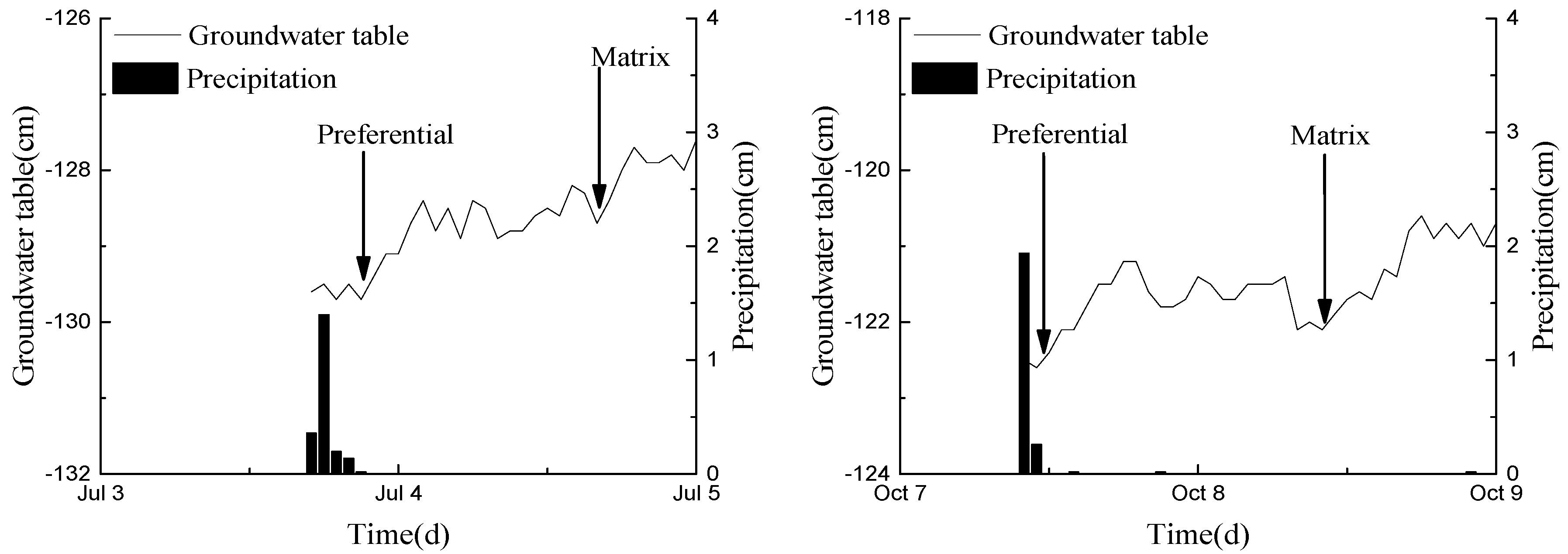Two field-measured water table series are plotted in Figure 12. Two different independent water table rising periods are clearly following rainfall while the rainfalls themselves are continuous. The first water table response may be the preferential flow and the second one is the matrix flow. The first response is the start of water table rising in field and the second is the following matrix flow. The response lag times of the matrix flow are 24 h on 3 July and 26 h on 7 October, respectively, corresponding to the modeled response lag times of groundwater recharge. According to Lee [44], this secondary response was more often in wetter seasons in which fissures can fill with water. Similar to Lee’s results, the secondary lagging often follows heavy and intense rainfalls in wetter periods. Only this time the root channels the preferential channel are rather than fissures.

In addition, the results of α values calculated by the model may be underestimated compared with α calculated by the observed data because we ignored preference flow in the numerical model. This underestimation effect and overestimation effect caused by ignoring lateral flow interacted, leading to results in Table 5. Preference flow was not obvious due to the huge soil water deficit in most infiltration events. But preference flow cannot be neglected in second heavy rains and third storm rains, which happened after sufficient precedent rainfalls (26.6 and 19.4 mm). Sufficient precedent rainfalls and relative high intensity, resulting in low soil water deficits and high-water content in the vadose zone, lead to a stronger preference flow. So calculated α was slightly smaller than observed in one of these two events, indicating that errors of ignoring preference flow overcame errors of ignoring lateral flow. Similar results were found in other rainfall events: smaller precedent rainfall leading to a smaller effect of ignoring preference flow in the calculation of α.

4. Conclusions

In this paper, the observed data and numerical model results were used to study the lag effects on precipitation infiltration recharge. The recharge coefficient of precipitation (RECOP) in this area was calculated by a numerical model; then the precipitation response depths, response lag time of water content and water table, invalid precipitation on the surface and at the water table were determined. It was noted that preference flow, dry sand layer, and cumulated precipitation effects on infiltration recharge should be considered in future research. The main conclusions are summarized as follows:

1. The test measurement data showed that the response depths of storm rain were more than 90 cm, while that of small rain were less than 10 cm, and both preferential flow and matrix flow existed in the study area. Measured groundwater recharge lag times (preferential flow) varied from 3 h–11 h.

2. In shallow groundwater areas of Mu Us Sandy Land, small rain cannot recharge groundwater. The RECOP was 0.47, that of heavy rain was 0.35–0.56, that of storm rain was 0.16–0.64. The total precipitation from March to November 2014 was 568 mm, and the total precipitation infiltration recharge was 268.8 mm, accounting for 47.3% of the total precipitation in 2014.

3. Based on in situ field monitoring data, the cumulative precipitation in the previous period reduced the lag time of water content but only affected on latter recharge within 144 h.

4. Invalid precipitation on the surface in shallow groundwater areas of Mu Us Sandy Land was 0.8–0.9 mm in 1 h. The invalid precipitation for groundwater recharge was 11.25–11.75 mm in 1 h when the groundwater depth was 120 cm, and 15–15.5 mm when the depth was 140 cm. Considering this, these high invalid precipitations can effectively improve accuracy of groundwater resources evaluation in semi-arid regions.

5. For middle rain, the modeled water content response lag time was 1 h at 10 cm, 10–12 h at 30 cm, 16 h at 60 cm, 25 h at 90 cm; for heavy rain, 1–2 h, 4–9 h, 13–16 h and 18–19 h, respectively; for storm rain, less than 1 h, 2–5 h, 3–12 h and 6–18 h, respectively. Modeled groundwater recharge lag times (matrix flow) varied from 11 h to 48 h. The lag time is non-negligible in groundwater recharge calculation, and this can provide scientific evidence for an aquifer’s response mechanism on human activities and climate change and sustainable groundwater resource utilization in semi-arid regions.