1. Introduction
It is important to assess how much uncertainties are involved in hydrologic modeling because there are many different sources of uncertainty including model structures, parameters, and input and output data [
1,
2,
3,
4]. Model structural uncertainty is due to the fact that we cannot perfectly represent the natural processes involved in hydrologic modeling [
4]. Parameter uncertainty indicates that many model parameters are not directly measurable (such as conceptual parameters) or can only be obtained with unknown errors (such as physical parameters) [
3]. Measurement uncertainty in input and output data can be caused by unknown measurement errors, incommensurability issues, etc., [
2,
4]. Uncertainty is either epistemic or aleatory [
5]. Epistemic uncertainty results from a lack of our knowledge while aleatory uncertainty arises from random variability. The former can sometimes be reduced by gathering more data and improving our knowledge while the latter cannot. A typical modeling process involves comparing the observed data with unknown errors (aleatory or epistemic) and model output that is simulated by an imperfect model with its own structural (epistemic), parameter (epistemic, aleatory, or both), and measurement (aleatory or epistemic) uncertainties. Since this process brings in different types of uncertainty in a non-linear and complex manner, it is very challenging, if possible at all, to disaggregate the observational error (difference between the observed and simulated variables) into different sources without making strong statistical assumptions about each source of uncertainty [
4]. For example, the parameter and input measurement uncertainties are propagated through the model structural uncertainty resulting in predictions with both epistemic and aleatory uncertainties, which are then compared to the observed data with its own uncertainty. The major problem with error disaggregation is that the observational error is not completely aleatory in nature and may not be appropriately modelled by a statistical model, which is often used to quantify aleatory uncertainty in random variables [
5].
The generalized likelihood uncertainty estimation (GLUE) method [
6] takes a different approach and does not strongly requires statistical assumptions on errors. This method has been widely used for uncertainty analysis in hydrologic modeling because of its simplicity, ease of implementation, and less strict statistical assumptions about model errors [
6,
7,
8,
9,
10,
11,
12,
13,
14,
15]. As its name implies, GLUE provides a general framework for uncertainty estimation and, unlike formal Bayesian methods, it does not require statistical assumptions about the structure of model errors although those assumptions may be made within the framework to use a formal likelihood function for statistical analysis [
16]. GLUE allows the use of an informal likelihood measure that evaluates the fitness of the model to the observed data. The likelihood measure is a function of the model parameters and observed data, whose value is rescaled to sum to 1 over the ensemble of behavioral models. The likelihood measures before and after incorporating information from the observed data are referred to as the prior and posterior likelihood, respectively. The prior likelihood is typically defined based on the modeler’s judgment and knowledge about the model and study area before incorporating information from the observed data. The posterior likelihood is obtained by multiplying the prior likelihood and the likelihood measure given the observed data as follows:
where
θ is the model parameter set,
ξ and
y are the observed input and output data, respectively,
is the likelihood of
θ given
ξ and
y,
and
are the prior and posterior likelihood of
θ before and after observing
ξ and
y, respectively, and
C is a normalizing constant such that the sum of
becomes 1. Parameter samples are classified as either “behavioral” or “non-behavioral” depending on their posterior likelihood and predefined threshold value. Behavioral models simulate output variables acceptably giving a likelihood value greater than a preset threshold value or within the limits of acceptability while non-behavioral models do not.
The prediction percentile of the behavioral models is defined as follows:
where
Z is the variable that the model predicts,
t is the time step,
is the predicted variable
Z at time step
t,
is the prediction percentile of the behavioral models predicting the variable
Z as less than
at time step
t, and
n is the number of behavioral models. For each time step, the prediction percentile is evaluated independently, and the lower and upper tails of the prediction percentile are abandoned to build uncertainty bounds with a certain confidence level.
Unlike probabilistic uncertainty estimation methods that try to fit statistical error models to input, output, or parameters in the hope of being able to justify those statistical characteristics of different errors, GLUE does not explicitly separate the observational error into different sources and, instead, focuses on evaluating the “effective observational error,” which is the deviation of model predictions from observed variables [
1]. Beven extended the concept of model evaluation to include set-theoretic approaches because traditional likelihood measures aggregate errors into a single performance measure in which errors in certain time steps can easily be compensated for by errors in other time steps [
1]. In set-theoretic model evaluation, at each time step during the simulation period, a fuzzy membership function is defined where the observed value takes a peak value of 1 and gets assigned the minimum and maximum acceptable limits of model predictions with a likelihood value of 0. A predicted value at each time step is assigned a membership value from this function. The shape of the membership function can vary depending on applications and available information. These limits of acceptable model predictions are referred to as the “limits of acceptability” in GLUE. Unlike aggregation-based approaches, set-theoretic approaches adopt fuzzy logic operators, especially fuzzy intersection or fuzzy AND, which is the minimum of all membership values. That is, the likelihood value of a model is the minimum membership value of all predicted values across the entire calibration period. Even if a predicted value at just one time step falls outside the limits of acceptability, this model is considered non-behavioral. Beven and Smith also discussed how to formulate a likelihood measure when there is disinformation in the data [
17]. In this research, they did not construct the limits of acceptability as a fuzzy membership function, but instead they used the absolute model residual and informative data to express a likelihood measure and assigned a likelihood of 0 to models that fail to predict any rainfall events during simulation. In this study, we refer to this method as the “absolute model residual method.”
There are different parameter sampling methods that have been used with GLUE including the nearest neighbor method [
6], a hybrid sampling strategy of the genetic algorithm and artificial neural network (GAANN) [
18], adaptive Markov Chain Monte Carlo (MCMC) sampling [
19], and uniform random sampling that is generally used with GLUE [
19], among others. One of recent sampling techniques used with GLUE includes the work of Cho and Olivera [
20]. They combined GLUE with a multi-modal heuristic algorithm called isolated-speciation-based particle swarm optimization (ISPSO) [
21] to introduce a hybrid uncertainty estimation method, ISPSO-GLUE. They applied the ISPSO-GLUE method to the Soil and Water Assessment Tool (SWAT) [
22] and compared ISPSO-GLUE and a random sampling version of GLUE using the Nash–Sutcliffe (NS) coefficient [
23] as the likelihood measure. They concluded that, with a faster convergence rate and a smaller number of parameter samples, ISPSO-GLUE only slightly underestimated the predictive uncertainty and likelihood-weighted ensemble predictions compared to GLUE using random sampling. They used the same likelihood measure for both methods, so the only differences between the two methods were the sampling method and how ISPSO-GLUE compensated for biased sampling. Since SWAT is a long-term hydrologic model that is computationally expensive, they conducted uncertainty analysis based on 46,000 parameter samples because of limited computational resources and time constraints. However, considering the 17 model parameters they changed during calibration, 46,000 samples might not have explored the parameter space comprehensively and so might not be enough to evaluate the performance of a large number of samples in the ISPSO-GLUE and GLUE methods. For example, a slight underestimate of predictive uncertainty in their study might have been due to a relatively small number of samples compared to the number of model parameters and ISPSO-GLUE may have not performed favorably if they took a lot more samples because of the effects of overly optimized (or overly conditioned on the calibration data) parameter values even with its compensation for bias. Cho et al. [
24] investigated the efficiency of the ISPSO-GLUE method in hydrologic modeling using the topography model (TOPMODEL) [
25] and the NS coefficient as the likelihood measure, and found that the cumulative model performance of ISPSO-GLUE converged much faster than GLUE with random sampling and its 95% uncertainty bounds contained 5.4 times more observed streamflows than those of GLUE. Their results showed that random sampling in GLUE initially performed better, but parameter sets from ISPSO-GLUE had improved at a much faster rate and reached an NS coefficient value of 0.82 compared to 0.47 by GLUE. We believe that this faster discovery of better behavioral models is one of the favorable characteristics of ISPSO-GLUE, but their simulation period was limited to only one year because of the lack of input and output data, and the number of parameter sets was 10,000. Also, they only assessed the NS coefficient as a likelihood measure.
Our first objective is to evaluate four likelihood measures including two limits of acceptability methods [
1] and two absolute model residual methods [
17] within the GLUE framework for TOPMODEL. Since the limits of acceptability and absolute model residual methods are more focused on rejecting models on a time-step-by-time-step (or event-by-event) basis rather than evaluating the models by aggregating individual observational errors from all time steps such as in the NS coefficient, it would be useful to see how these approaches perform in a long-term hydrologic simulation because we believe that the longer the simulation period is the harder it would be to find behavioral models that can make predictions within the limits of acceptability across the entire period. In fact, we reported total failures of these methods at least for our study area and discussed our findings.
The second objective is to compare ISPSO-GLUE and GLUE to observe how each method performs when the number of samples becomes a lot larger (half a million) than 46,000 with SWAT [
20] and 10,000 with TOPMODEL [
24]. We used random sampling with GLUE because, compared to most of other sampling techniques, this method has an advantage that the modeler does not need to modify the likelihood to reflect non-uniform sampling results [
5] and unbiased uniform samples can serve as a reference population for performance comparisons with other uncertainty analysis methods. We compared the performance of ISPSO-GLUE and GLUE in terms of the wall-clock time [
26] of simulations, convergence rate, and percentage of enclosed observed data. Finally, we examined samples in the parameter space from both methods to see how well the ISPSO-GLUE samples explored and exploited the problem space, and assessed the applicability of ISPSO-GLUE to the uncertainty analysis of TOPMODEL.
In this study, we did not try to construct unknown statistical models to consider different sources of uncertainty in GLUE explicitly because doing so could easily overestimate information content in the observed data. Instead, we made a subjective assumption that informal likelihood measures implicitly incorporate these uncertainty sources. We also examined the impact of widening the limits of acceptability (adding more uncertainty) on the result of uncertainty analysis.
3. Results and Discussion
3.1. Limits of Acceptability and Absolute Model Residual Methods
All four methods with GLUE (Equations (17)–(20)) found no behavioral models at all for the calibration period and, consequently, for the validation period as well. In other words, for all four approaches, not a single model out of a half million random samples was able to simulate flows within the acceptable error deviation for all time steps. We found that it would be very challenging for one model to be able to simulate flows for 5 years or 1826 days within certain limits of acceptability at all times. There are dry and wet seasons during the time of a year and a similar pattern repeats five times. A single set of the model parameters may perform well in either a dry or wet season, but that performance does not guarantee a similar efficiency in the other types of flow seasons.
Specifically, the constant error deviation estimator
in Equation (15) was not able to explain error variations across different flow seasons.
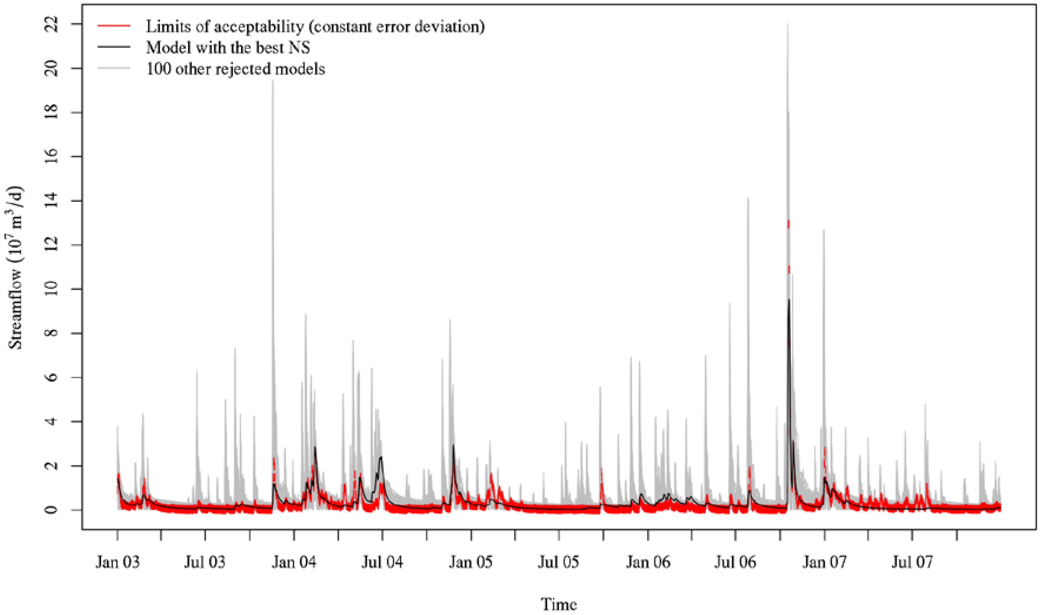
Figure 2 shows the simulated streamflows from the best NS and 100 other rejected models along with the limits of acceptability using the constant error deviation. As can be seen in this figure, TOPMODEL either highly overestimated or underestimated peak flows and simulated flows often fell outside the acceptable limits defined by the error estimator. The lack of any behavioral models may be attributed to the fact that we did not explicitly consider uncertainties in other sources than the observed data in the likelihood measure itself. We examined how much the acceptable range should be expanded to classify the model with the highest NS coefficient value (the “best” model) as behavioral. We divided the absolute error by the constant error deviation estimator to compute the error ratio relative to the error estimator (ER). About 28% of all time steps were found outside the acceptable range (ER > 1). Even after stretching the acceptable range two times wider, we found about 11% of all time steps outside the wider acceptable range (ER > 2). The largest deviation of the simulated flow from the observed flow was about 23 times larger than the error estimator (ER ≈ 23). However, this largest deviation relative to the error estimator occurs at the highest peak flow and does not necessarily mean that the model failed to simulate other time steps altogether. We found that we needed to widen the acceptable range 2.1 times the initial range to find about 90% of time steps within the widened acceptable range. However, even in this case, about 10% of the time, simulated flows fell outside the 2.1 times wider acceptable range. In other words, incorporating more uncertainties from other sources into the acceptable range implicitly by expanding it by 2.1 times would not result in any behavioral models either. Provided that the constant error deviation estimator is 65.6 times greater than the mean observed data and 1.3 times greater than the maximum observed data, more than doubling the observational error to implicitly consider other sources of uncertainty might overestimate the total uncertainty. That is, even explicitly incorporating other sources of uncertainty into the acceptable range might have not resulted in any behavioral models either even after ignoring the 10% worst simulated flows. We needed to expand the limits of acceptability by 23 times to find any behavioral models. The non-parametric error deviation estimator
in Equation (16) tries to estimate error deviations locally using local information at any time step in the observed time series. However, when there are very similar flows in consecutive time steps, the error estimator estimates a very small error deviation, which makes it even more challenging to accept any model as behavioral.
The two absolute model residual methods in Equations (19) and (20) were not very different in this regard. As mentioned above, the reason why all models were rejected as non-behavioral might be attributed to a long simulation period of 5 years, so we conducted another set of experiments using the two absolute model residual methods for two sets of 1-year calibration (2003 and 2004) and validation (2009 and 2010). However, the results for these simulations have not produced any behavioral models either. For these methods, we estimated the time of concentration as 112 hours or 4.7 days using the TR-55 method for identifying disinformative data. For comparison, we calculated this hydrologic parameter using the best behavioral model from ISPSO-GLUE (NS = 0.80). The internal subcatchment routing velocity vr was found to be 1038 m/h. By dividing the longest flow path 124 km by this routing velocity, we obtained the time of concentration of 119 hours or 5 days. Even using daily time steps, TOPMODEL agreed well with the TR-55 method within a 7% difference when estimating the time of concentration. We believe that this cross validation between TR-55 and TOPMODEL, and 5 days of the time of concentration, imply that the coarse daily temporal scale had minimal impacts on the estimated contributing areas.
This total failure of the four likelihood methods might have revealed the weakness and challenge of evaluating model predictions using the fuzzy AND operator (the minimum likelihood of all time steps), especially in long simulations in such a restrictive way. At the same time, it brings up a question about how we can effectively incorporate input uncertainty into the effective observational error without making unjustifiable statistical assumptions about the structure of the input error. All these questions are left for future research at this point.
We did not run ISPSO-GLUE using these four likelihood methods in this study. Unlike random sampling for GLUE, in case of ISPSO-GLUE, since parameter samples (particles) respond differently to different objective function surfaces, it is necessary to conduct separate optimization runs using these likelihood methods for comparing ISPSO-GLUE and GLUE, but limited computational resources and time constraints prohibited us from performing this comparison using the limits of acceptability. However, it is not impossible to run ISPSO-GLUE using this fuzzy-set-based objective function with one modification. Unlike random samples that are independent on each other, particles from ISPSO-GLUE depend strongly on information from their own past experience and other particles when evolving, and identification of “better” models with a higher likelihood measure is a crucial requirement for the exploration and exploitation of the search space. With the current limits of acceptability, two non-behavioral models would get assigned a likelihood measure of 0 and an optimization run would not be able to tell in which direction particles should evolve. This information loss occurs because the limits of acceptability function is truncated at 0. The fuzzy membership function (limits of acceptability function) would need to be extended below 0 indefinitely to be able to “sort” the performance of non-behavioral models to produce the necessary information for swarm evolution. Investigating this simulation is left for future research.
3.2. Wall-Clock Time of Simulations
At the end of each method, the total wall-clock times were 725 min for ISPSO-GLUE and 730 min for GLUE. The mean run times per model run were 0.087 s for ISPSO-GLUE and 0.088 seconds for GLUE. GLUE was marginally faster than ISPSO-GLUE until about 364,000 model runs, but later ISPSO-GLUE became slightly faster than the GLUE method. On average, the overhead by particle evolution was almost negligible at the beginning and ISPSO-GLUE finished its simulation about 5 min earlier than GLUE. The wall-clock times of both methods were comparable and may not be one of major factors when choosing ISPSO-GLUE over GLUE.
3.3. Model Performance
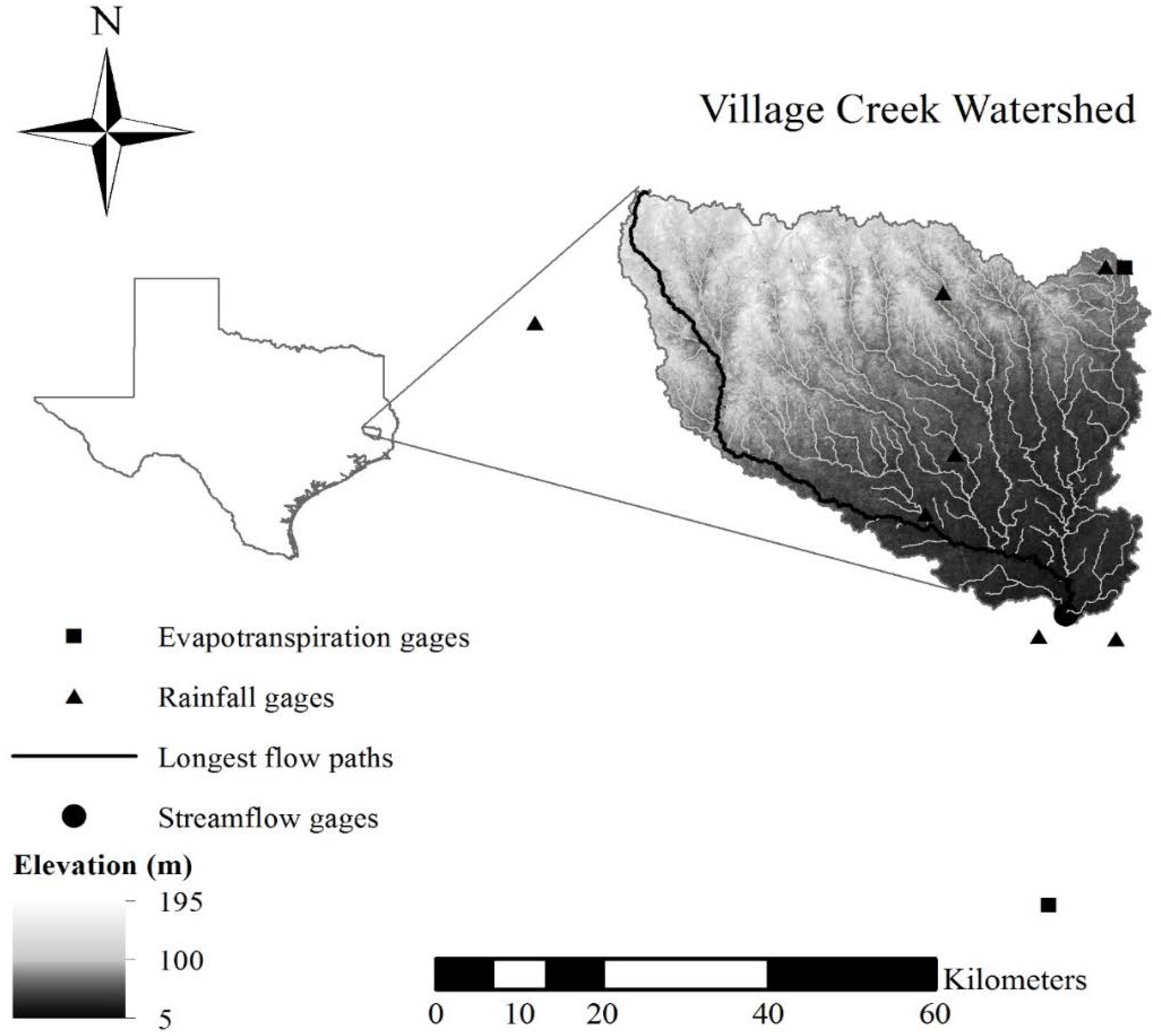
Since a half million random samples failed to make predictions with the limits of acceptability and absolute model residual methods, at this point we asked ourselves if those samples would really be all useless in estimating predictive uncertainties in hydrologic modeling for the Village Creek watershed. We believe that it is a valid question because we obtained decent NS coefficient values for the same 5-year simulation (2003–2007 with GLUE).
Table 2 summarizes the results of ISPSO-GLUE and GLUE. As can be seen in this table, the maximum NS coefficient was 0.80 for the 5-year GLUE calibration and the number of behavioral models was 28,289 out of a half million. The NS coefficient is an aggregated performance measure where it summarizes all simulated flows and observed flows in a single performance index rather than treating those simulated flows individually and taking the worst performing simulated flow as the representative performance measure just like in the limits of acceptability approach. For this reason, any periods where the model performs poorly can be compensated for by other periods where the model performs very well. This kind of performance compensation may not be acceptable for the limits of acceptability approach, but, sometimes, we may not be able to afford to reject a half million models as non-behavioral just because some portions of the entire simulation period were not simulated acceptably. In this study, we made that compromise and chose to use the NS coefficient as the likelihood measure to compare the two uncertainty analysis methods.
However, even the NS coefficient approach has produced a small number of behavioral models only for 3 out of 5 calibration periods for GLUE (1.3% to 5.7% of all model runs) and both methods failed to find any behavioral models for the 2003–2004 and 2003–2005 simulations. ISPSO-GLUE found a lot more behavioral models for the same calibration periods (98.3% to 99.5% of all model runs), but most of those models were found around a small region of the search space, especially on the axes of a few sensitive parameters such as lnTe, m, and vr, which will be discussed later in
Section 3.4.
ISPSO-GLUE required up to two orders of magnitude fewer model runs to obtain a similar NS coefficient when both methods found any behavioral models. GLUE outperformed ISPSO-GLUE in terms of the percentage of enclosed observed flows at the expense of more model runs, but the maximum NS coefficients for both methods were comparable. The mean observed flow for the 5-year calibration period (2,598,131 m3/d) is more than two times that for the 5-year validation period (1,124,422 m3/d). Also, the variability of the observed flow in the calibration period is much higher than in the validation period. These two simulation periods exhibit very different characteristics of the observed time series and those models that performed well in the calibration period have failed to show similar performance in the validation period for this reason. However, running all half a million random models—not just those behavioral models from the calibration period—in the validation period has produced the maximum NS coefficient of 0.45 for the GLUE method, which is smaller than the threshold NS value of 0.6. In other words, for the GLUE method, if we used the validation period (2009–2013) for calibration, we would have obtained no behavioral models at all from half a million random samples and there would be no behavioral models left to simulate the validation period (2003–2007). We performed a separate set of optimization runs using ISPSO-GLUE for the validation period and obtained the maximum NS coefficient of 0.45. This result confirms that the performance of TOPMODEL in the validation period may not exceed the threshold NS coefficient of 0.6.
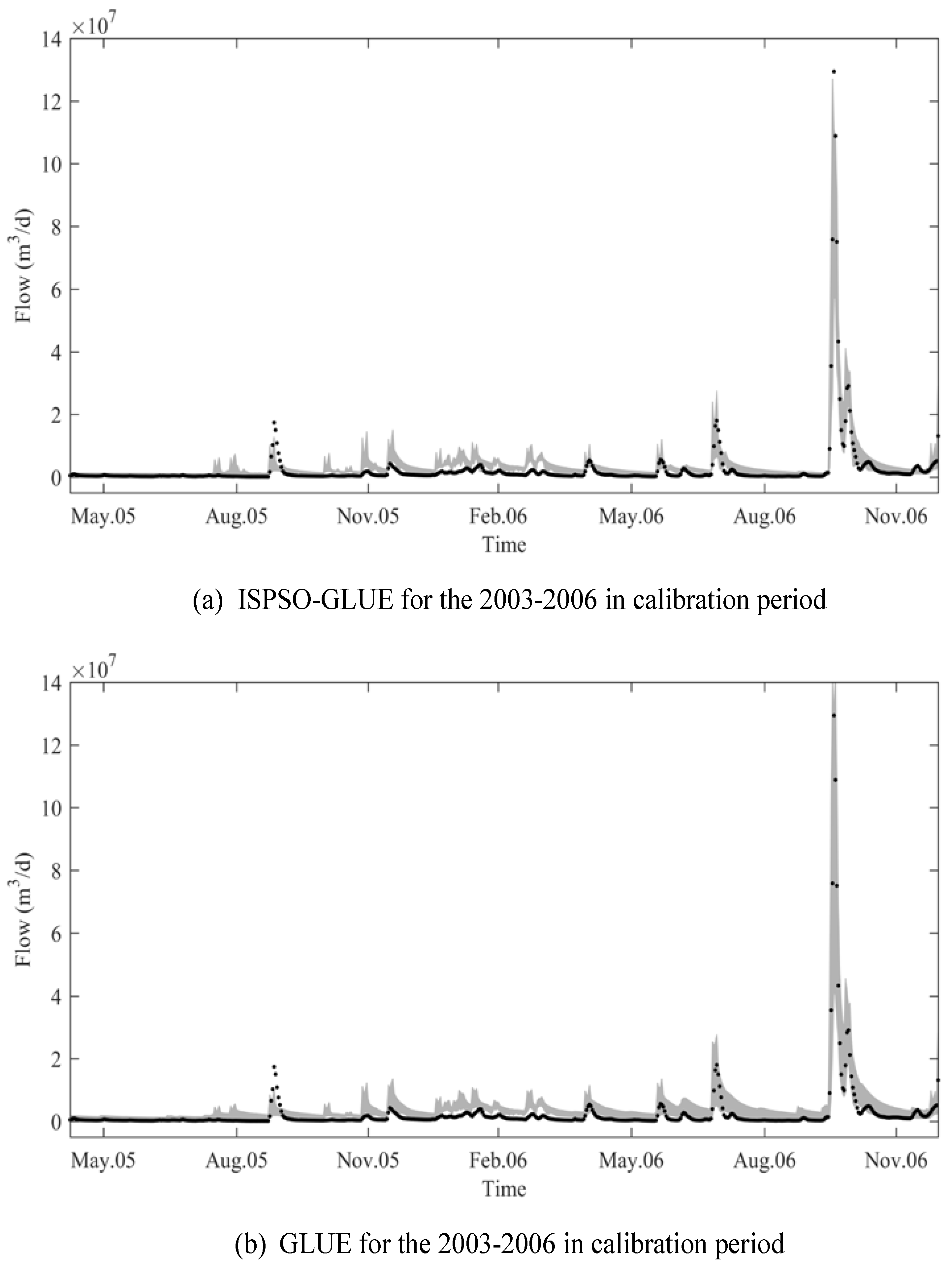
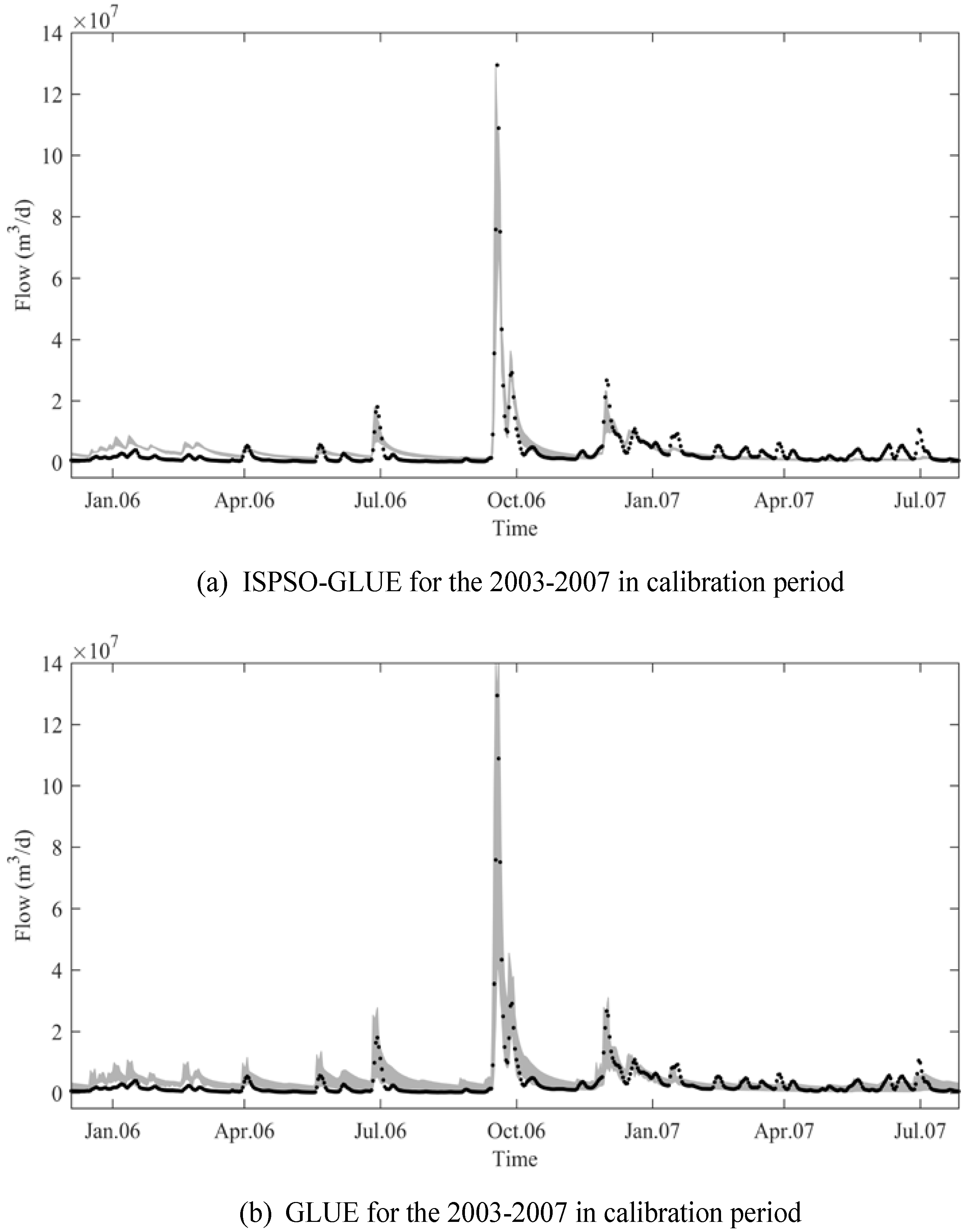
The major increase in model performance between the 2003–2005 and 2003–2006 calibration periods can be explained by the highest peak flow on 19 October 2006 and the higher mean observed flow because of this peak flow. A higher NS coefficient indicates that a model performs relatively better than the mean observed flow. As shown in
Figure 3 and
Figure 4, both methods predicted the peak flow really well while they did not perform well during the low flow seasons. Since the peak flow was well simulated, its squared residual did not contribute much to the sum of squared residuals in the numerator of Equation (21) while it increased the mean observation and, consequently, the denominator. As a result, the NS coefficient increased significantly, but it does not mean that both methods made good predictions even during the low flow seasons. We could have excluded these high peak flows from NS evaluation from the beginning and rejected all models as non-behavioral based on lower NS coefficient values. This strategy is well aligned with the concept of disinformative data in the absolute model residual methods. Using only informative data to evaluate the NS coefficient after filtering out extremely high peak flows may address this issue with the NS coefficient, but, in our study, we did not explore this NS coefficient approach with informative data only because of computational and time constraints. However, we believe that this approach is worth an investigation in the future.
Overall, the performance of the behavioral models was not great because validation has failed for all five simulation periods. This result was unexpected in the beginning because we assumed that half a million samples should be enough to generate behavioral models for those five sets of calibration and validation periods at least for the GLUE method. For the ISPSO-GLUE method, half a million particles may have been over-conditioned to the calibration data, which can result in poor performance in the validation period. Comparing the maximum NS coefficients for the validation periods between the two methods, we found weak evidence of over-conditioning of particles to the calibration data because ISPSO-GLUE performed marginally worse than GLUE for all validation periods (difference in NS varies from −0.04 to −0.02). However, at the same time, ISPSO-GLUE enclosed fewer observed flows than GLUE did. This observation reveals that finding most models from favorable regions of the search space and weighting them based on the inverse geometric mean of the number of samples may not adequately address the over-sampling bias caused by selective sampling through optimization. The threshold value for the NS coefficient of 0.6 might have been too high when the highly wet period in 2006 inflated the NS coefficient for 2003–2006 and 2003–2007. However, the threshold value represents the modeler’s expectation before analysis and we believe that lowering the threshold value just to obtain more behavioral models is not the correct way to perform uncertainty analysis. The failure of validation for all simulation periods suggests that other likelihood measures might work better for this specific watershed or a rather coarse daily time step due to limited available data may have affected surface runoff produced by infiltration excess or saturation excess. This complete failure in validation can also mean that the model structure of TOPMODEL might not be good enough to describe this catchment. We observed one potential problem in how TOPMODEL routes the total flow to the outlet. If the main channel within a subcatchment is long enough that more than one time step is required to drain the flow, the contributing area of the subcatchment is divided proportionally to the time step. As a result, the flow generated within the subcatchment is also divided in the same way and routed to the outlet. This proportional contribution of the total flow may or may not work depending on the structure of the stream network within the subcatchment and increases the model structural uncertainty in the simulated output.
3.4. Behavior of Parameter Samples
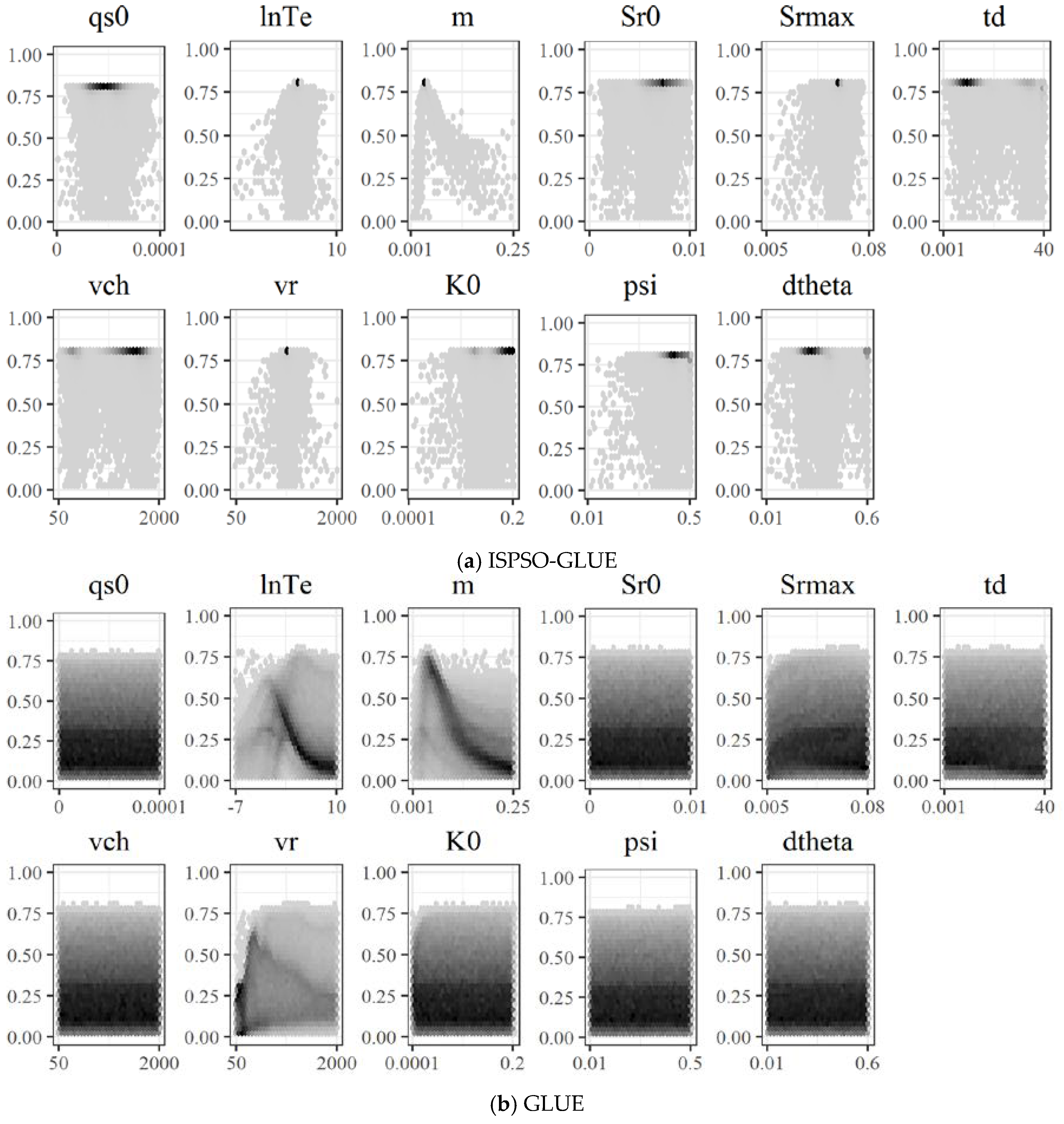
The objective function surface needs to be examined to investigate how sensitive the model performance is to parameter values. We used the 5-year calibration and validation periods for this analysis because both methods performed well in the calibration period. Because the dimension of the problem is 11, two-dimensional projections of the objective function surface are presented as the hexagonal bin plots [
56] of NS versus each parameter as shown in
Figure 5. We chose to plot samples on a hexagonal bin plot because there are half a million points that overlap significantly in a small scatterplot and cannot be represented well in terms of densities if they were plotted individually. For our study, a hexagonal plot was created by first drawing imaginary hexagons in the 2-dimensional space of the NS coefficient versus each parameter, counting the number of samples falling in each hexagon, and color-coding those hexagons with some samples. The color of the hexagons represents the sample density.
Figure 5b shows the parameter distributions of random samples from GLUE, which represent the overall shape of the parameter space better than those of selective particles from ISPSO-GLUE as shown in
Figure 5a.
The parameters lnTe, m, and vr showed a similar tendency of random samples clustering around a certain value. The parameter Srmax performed worse closer to the lower limit, but overall, the model performance was not highly sensitive to this parameter. Comparing the two sets of hexagonal bin plots for ISPSO-GLUE and GLUE, we can clearly see that random samples in GLUE were more likely to cluster around regions of low likelihood, as the bottom portion of the plots in
Figure 5b is much darker than in
Figure 5a. At the same time, particles from ISPSO-GLUE show a tendency to move toward regions with higher likelihood as darker hexagons are more focused around the maximum NS coefficient. In other words, most random samples in GLUE were found in regions of low likelihood while particles in ISPSO-GLUE explored and exploited the search space in regions of high likelihood. Another important observation is that the lnTe, m, and vr parameters exhibit single modality in general, which causes particles from ISPSO-GLUE to cluster around a small region of single optimal parameter values in the search space. This particle behavior reduces the diversity of behavioral models significantly and limits the width of uncertainty bounds, which will be discussed later.
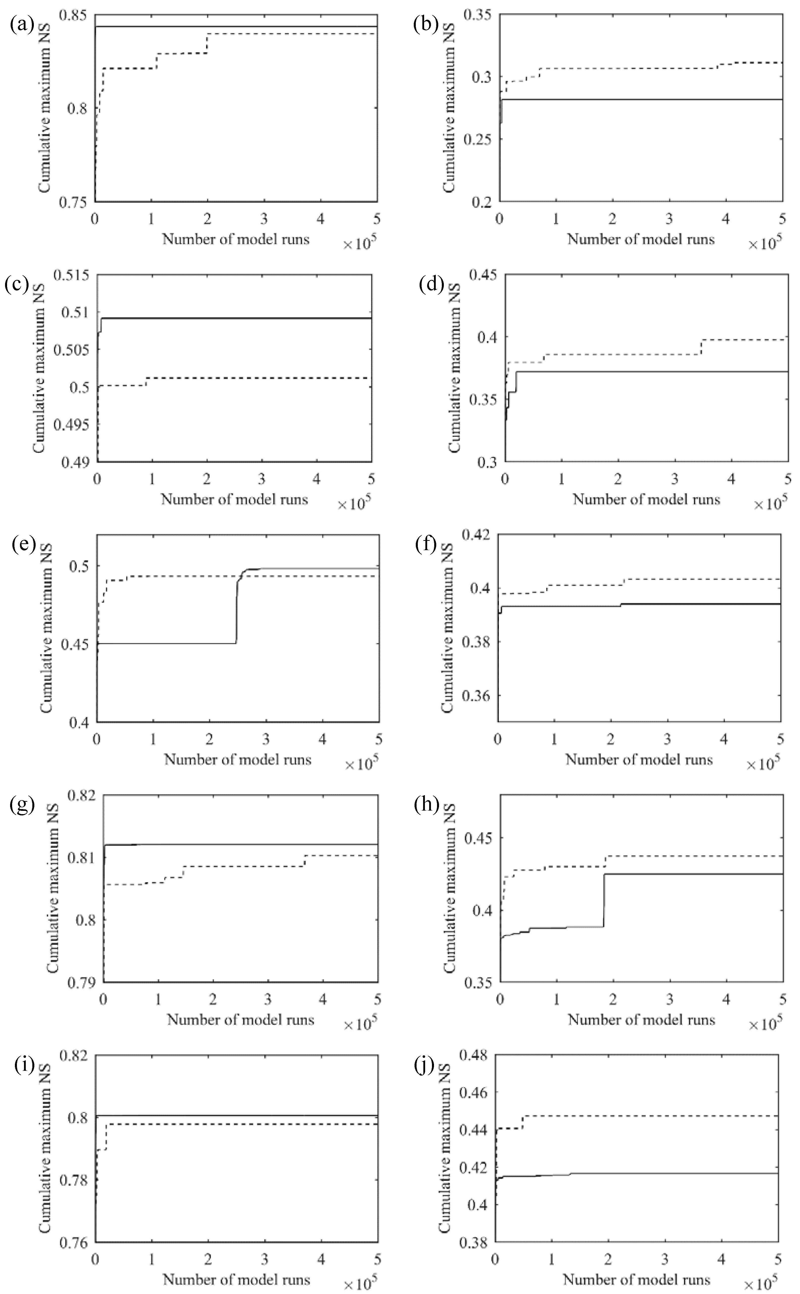
Figure 6 shows the convergence rate of the NS coefficient with respect to the number of model runs for different simulation periods. The validation plots were created using both behavioral and non-behavioral models to see how both methods perform as the number of model runs increases. The cumulative maximum NS coefficient is obtained from the best model found so far at each iteration and indicates how fast the performance of each method converges to the final state. Overall, the convergence rate of ISPSO-GLUE was faster than GLUE. Although ISPSO-GLUE found better samples than GLUE at the very beginning of the simulation in the 2003–2005 calibration as shown in
Figure 5e, GLUE took a small number of model runs to move ahead of ISPSO-GLUE. After about 250,000 model runs, ISPSO-GLUE started outperforming GLUE. This observation suggests that taking random samples from the parameter space can be more beneficial initially until the strategic evolution of particles reaches an optimal solution eventually. To investigate the effect of randomness in sampling on the performance, a bootstrapping analysis without replacement was conducted 1000 times with the GLUE samples for the 3-year calibration period. All re-sampled parameter sets exceeded the performance of ISPSO-GLUE before about 5000 model runs. However, after the initial discovery of a good solution, GLUE had never experienced a significant performance improvement afterward. This analysis shows that random sampling may find good solutions early by luck depending on the landscape of the objective function surface, but it takes more strategic efforts to explore the search space and find better optimal solutions. The number of model runs in ISPSO-GLUE to exceed the performance of GLUE depends on the study area and hydrologic data used. For example, for the Village Creek watershed, the number of required model runs in ISPSO-GLUE varied from 250,000 runs for the 3-year calibration period to less than 1000 runs for the other calibration periods.
3.5. Uncertainty Bounds
The number of behavioral models in
Table 2 shows biased sampling of ISPSO-GLUE towards optimal solutions with more than 98% of 500,000 models being behavioral while GLUE only found 1%–6% in the calibration periods. Because of a sampling bias in ISPSO-GLUE, the higher number of behavioral samples does not necessarily mean that this method has found that many unique samples that are significantly different from each other. However, the “nesting radius” in ISPSO makes sure that no samples are duplicated within this distance. Also, the weighting method in Equation (3) penalizes highly dense regions with a lot of samples that are similar.
As can be seen in
Table 2, even with more behavioral models, the uncertainty bounds for ISPSO-GLUE enclosed less observed flows as compared to those for GLUE. The average percentages of enclosed observed flows for ISPSO-GLUE and GLUE are 16.6% and 30.2%, respectively. Overall, the ISPSO-GLUE uncertainty bounds enclosed 13.6 pp (percentage points) less observed flows than the GLUE uncertainty bounds. However, Cho et al. [
24] found contradictory results using TOPMODEL for another Texas watershed during a dry period where ISPSO-GLUE enclosed 79 pp more observed daily streamflows than GLUE. Behavioral models in their GLUE method using random sampling performed worse than those in the ISPSO-GLUE method because of low baseflows. In this study, this relative performance of the uncertainty bounds is reversed and GLUE performed better than ISPSO-GLUE. One of the major differences between this study and their study is the total number of samples. Compared to their study, the total number of samples is 50 times larger, and evolving the particle swarm 50 times more can result in extremely highly populated regions with good likelihood. These over-populated regions can give too much weight to good simulations, which closely simulate observed flows, but may not encompass a lot of them together as an ensemble. In other words, behavioral models from GLUE showed a higher variability than those from ISPSO-GLUE and produced highly variable model outputs with small to large errors surrounding the observed flows. This higher variability of the performance of GLUE was translated into wider uncertainty bounds, which enclose more observed flows.
Figure 3 and
Figure 4 show the 95% uncertainty bounds for the wettest period of the 4-year and 5-year calibration periods, respectively. The ISPSO-GLUE uncertainty bounds were generally narrower and missed extreme peak flows as compared to those of the GLUE method. These plots show that, even if ISPSO-GLUE produced uncertainty bounds with a narrow prediction band, and their predictive accuracy was not high enough to enclose a reasonable amount of the observed data when compared to GLUE. This result clearly reveals the weakness of a hybrid uncertainty analysis method like ISPSO-GLUE, where samples are taken to calibrate the model parameters as well as to perform uncertainty analysis. The result presented in this study is less desirable than the result of Cho and Olivera [
20] using SWAT, which is highly multi-modal with many spatially distributed parameters.
Figure 5 shows the single modality of TOPMODEL in the parameters lnTe, m, and vr, and the insensitivity of the other parameters to the NS coefficient. While single modality makes it easier to calibrate the model parameters, it reduces the diversity of particle sampling once the optimization algorithm found the global solution. Reduced diversity in parameter sampling can lead to low variability in simulated flows in ensemble predictions and cause the uncertainty bounds to miss more observed data.
3.6. Suggestions
Particles from the ISPSO-GLUE method successfully identified sensitive parameters and found regions with behavioral models. However, the strategic evolution of the particle swarm resulted in over-sampling of good behavioral models around preferable solutions even with low-discrepancy sampling, which increases the diversity of samples across the parameter space. Weighting the likelihood measure based on the population density of particles somehow alleviated the adverse effects of over-sampling bias, but the small variability of their high performance led to smaller intervals of the uncertainty bounds compared to those of the GLUE uncertainty bounds. On average, ISPSO-GLUE enclosed about 13.6 pp less observed data than GLUE did. It does not necessarily mean that ISPSO-GLUE will always enclose a lot less observed data than GLUE as shown by Cho and Olivera [
20] and Cho et al. [
24], but it is advised that the objective function surface be closely inspected after an ISPSO-GLUE run to interpret and understand the uncertainty analysis results of the ISPSO-GLUE method. Since the single modality of the objective function surface adversely affects the performance of ISPSO-GLUE, the likelihood weighting method should be improved to gain better coverage of the observed data while particle samples are allowed to find optimal solutions. Lastly, it would be worth trying to evaluate an aggregated likelihood measure without disinformative data so that any extreme or abnormal hydrologic responses to forcing data do not highly affect the single index of the model performance in an adverse manner.
4. Conclusions
We investigated the use of four likelihood approaches with GLUE including two limits of acceptability and two absolute model residual methods. Half a million random samples were used to evaluate the four likelihood approaches. All these methods did not produce any behavioral models because it was very challenging for any models to make predictions within the acceptable effective observational error for all time steps. This failure highlighted the challenge of the limits of acceptability approach, especially in long simulations, and moved our attention to how we can better take into account different sources of uncertainty in model evaluation without strong statistical assumptions.
We also examined the applicability of ISPSO-GLUE to TOPMODEL by comparing its results to those of GLUE. A half million samples were taken randomly for the GLUE method to provide unbiased random reference samples for comparison and the same number of samples were generated by ISPSO. We used the NS coefficient for comparing the ISPSO-GLUE and GLUE methods. We split 10 years of data into 5 sets of calibration and validation periods, and performed ISPSO-GLUE and GLUE with random sampling for each calibration period. Behavioral models found during calibration were evaluated for the validation period. ISPSO-GLUE was able to identify sensitive parameters, but both methods failed to find any behavioral models for the 2–3 years’ calibration periods. More importantly, both methods failed in all the validation periods given an NS coefficient value of 0.6 as the behavioral threshold, which suggests that other likelihood measures might work better for this watershed or TOPMODEL might not be good enough to describe our watershed. For calibration, it was shown that random sampling may perform better in the beginning because of uniformly distributed samples, but after a certain number of iterations, particles in ISPSO-GLUE started outperforming the random samples with the help of strategic evolution of the particle swarm. ISPSO-GLUE achieved similar performance to GLUE in terms of the maximum NS value with up to two orders of magnitude fewer model runs for the simulations with any behavioral models. However, the uncertainty bounds of ISPSO-GLUE were generally narrower than those of GLUE and, consequently, its uncertainty bounds enclosed 13.6 pp less observed flows on average as compared to the GLUE uncertainty bounds. These relative differences were mainly caused by different parameter sampling strategies employed by the two methods that are highly affected by the shape of the objective function surface, and the length and characteristics of observed data. While the GLUE method randomly takes parameter samples from the search space, the ISPSO-GLUE method takes more samples from regions with high likelihood in the parameter space, leading to a much smaller variability of their model outputs and, hence, narrower uncertainty bounds. The single modality of TOPMODEL for the study area exaggerated this effect as compared to a similar study using SWAT, which exhibits multi-modality.
These findings suggest that an uncertainty analysis method for hydrologic modeling should be chosen carefully by considering the hydrological properties of the study area and observed data, because all these factors eventually affect the landscape of the objective function surface and the uncertainty bounds. At the same time, since the choice of a likelihood measure also strongly affects the performance of calibration and validation, other likelihood measures will need to be evaluated including aggregated performance measures without disinformative data and different limits of acceptability approaches. Future work on the ISPSO-GLUE method will include addressing the small variability of simulation outputs by further diversifying the search for single-modal problems and the investigation of the time complexity depending on its optimization parameters.


