Article

Optimizing the Water Treatment Design and Management of the Artificial Lake with Water Quality Modeling and Surrogate-Based Approach

1
POWERCHINA Chengdu Engineering Corporation Limited, Chengdu 610072, China
2
College of Environment and Civil Engineering, Chengdu University of Technology, Chengdu 610059, China
3
State Key Laboratory of Geohazard Prevention and Geoenvironment Protection, Chengdu University of Technology, Chengdu 610059, China
4
Institute of Water Sciences, College of Engineering, Peking University, Beijing 100871, China
*
Author to whom correspondence should be addressed.
Water 2019, 11(2), 391; https://doi.org/10.3390/w11020391
Submission received: 28 December 2018 / Revised: 16 February 2019 / Accepted: 19 February 2019 / Published: 23 February 2019
(This article belongs to the Section Water Quality and Contamination)

Abstract

:
The tradeoff between engineering costs and water treatment of the artificial lake system has a significant effect on engineering decision-making. However, decision-makers have little access to scientific tools to balance engineering costs against corresponding water treatment. In this study, a framework integrating numerical modeling, surrogate models and multi-objective optimization is proposed. This framework was applied to a practical case in Chengdu, China. A water quality model (MIKE21) was developed, providing training datasets for surrogate modeling. The Artificial Neural Network (ANN) and Support Vector Machine (SVM) were utilized for training surrogate models. Both surrogate models were validated with the coefficient of determinations (R2) greater than 0.98. SVM performed more stably with limited training data sizes while ANN demonstrated higher accuracies with more training samples. The multi-objective optimization model was developed using the genetic algorithm, with targets of reducing both engineering costs and target aquatic pollutant concentrations. An optimal target concentration after treatment was identified, characterized by the ammonia concentration (1.3 mg/L) in the artificial lake. Furthermore, scenarios with varying water quality in the upstream river were evaluated. Given the assumption of deteriorated upstream water quality in the future, the optimal proportion of pre-treatment in the total costs is increasing.

1. Introduction

The artificial lake at the city center is an integral and glamorous component of municipal landscapes, which plays a key role in the water quality management, ecological maintenance and contamination control [1,2]. The water environment conservation of artificial lakes has attracted considerable attention from governments and has huge market potentials, guided by the Chinese policy of environment conservation. Artificial lakes have high engineering plasticity, which means lake parameters could be adjusted flexibly due to intense human intervention and limited watershed scales [3]. However, at the present stage, the calculation of engineering costs for artificial lake design mainly concerns aesthetics and water quality without considering the interactions between costs and other design parameters. Therefore, reliable and accurate designs and decision-making based on robust quantification are necessary instead of just referring to experiences and subjective judgments.
Physically based numerical water quality models and optimization play an increasingly important role in the engineering design of artificial lakes because of their abilities to provide accurate and reliable proposals [4]. However, incorporating optimization with complex physically based numerical models would be extremely time-consuming, and thus this scheme is not widely used for engineering problems. Therefore, surrogate modeling, which mimics the behavior of complex numerical models with much computationally cheaper mathematical relationships, becomes a more suitable solution for optimization problems [5,6]. Using surrogate models, the computation cost of numerical models only concentrates on the training step, which could save considerable computation costs compared with directly using numerical models for optimization. Likewise, the real-time simulation for emergencies of water quality management also needs a surrogate model calculation to meet the extremely limited time requirement. Recent studies show that using surrogate models for the optimization based on numerical models has been a promising direction, which has higher extensibility and flexibility in selecting variables and better-calibrated models with a lower uncertainty [4,7].
Machine learning has been widely applied for training surrogate models in hydrological processes and water resources management issues [4,6]. The Artificial Neural Network (ANN) and Support Vector Machine (SVM) are two of the most popular and powerful algorithms [8]. The structure of ANNs is developed from imitating the communication systems of human neurons, which is able to learn general rules from training data by determining the connection weights between neurons [9,10]. ANNs have been used in soft-computing-based model construction for simulating water qualities [11,12,13], groundwater levels forecasting [14,15,16] and hydrological model parameter estimation [17]. The SVM is a two-layer structure including a nonlinear kernel weighting on input variables and a weighted sum of the kernel outputs based on the statistical learning theory [18,19]. SVM has also been widely applied in predicting river discharges [20], estimating groundwater pollution [21], simulating rainfall-runoff production [22]. However, few applications were reported for urban water quality management optimization using surrogate models trained by ANNs or SVMs because the management of urban artificial lakes is a newly developing area. ANNs implement the empirical risk minimization principle to minimize the training error while SVMs implement the structural risk minimization principle to minimize the upper bound of the generalization error [19]. Although SVMs were reported more efficient due to its higher generalization ability than ANNs [23], the criteria of selecting ANNs and SVMs have still not been determined when applying to specific problems, especially for the artificial lake design.
The combination of surrogate models and multi-objective optimization provides promising opportunities to solve tradeoff problems [24], e.g., maximizing water treatment abilities while minimizing construction cost at the same time. A set of alternatives (comprising the Pareto optimal solutions and the Pareto front) were generated by multi-objective optimization, which means no solution could be further improved according to both objectives [25,26]. The Pareto-optimal solutions yielded by genetic algorithms (GAs) need a huge number of iterations. Therefore, considering multiple demands and limited computational time, optimization models based on surrogates and GAs are preferred to reach the Pareto front [27]. The Pareto-optimal curve exported by multi-objective optimization can provide a multi-dimensional mapping relationship between decisions and results, which has stronger practical implications to decision-makers than that by the single-objective optimization.
In the present study, an artificial lake in a developing urban area was taken as an example, and surrogate models built based on a physically based numerical water quality model and coupled with multi-objective optimization were used to support decision-making on the water quality management and engineering designs. The study aims to seek an optimal scheme of economic efficiency and corresponding target pollution concentrations, supplementing the recognition of sphere of the intelligent system application and providing a case of water environment management with surrogate models and multi-optimization.

2. Modeling Roadmap

The overall roadmap is presented in Figure 1. The three major parts in the framework are the numerical model construction, surrogate model training, and multi-objective optimization modeling. The calibration of the numerical model and sensitivity analysis are conducted to guarantee the accuracy of simulation and the representativeness of selected input variables. After the batch operation of the numerical model, a set of input–output data are generated to train surrogate models, with an ANN and an SVM being used to conduct the training step. In the step of optimization modeling, the minimum engineering costs and minimum pollutant concentrations of lake water are set as objectives. The validated surrogate models can precisely interpret the nexus between input variables and output water quality indicators, while the nexus between input variables and the total cost can be deduced through the cost estimation. Then, the Pareto-optimal solutions calculated by the multi-objective optimization using a GA can demonstrate the tradeoff between different objectives.

2.1. Introduction to MIKE21

MIKE21 (DHI, Copenhagen, Denmark) is a physically based numerical hydrodynamic and water quality model developed by the Danish Hydraulic Institute (DHI) (https://www.mikepoweredbydhi.com/). In this study, the two-dimensional computer program MIKE21 was used to build the numerical model in the roadmap. MIKE21, coupled with the ECO Lab (DHI, Copenhagen, Denmark) module, was used to simulate the hydrodynamic and water quality processes of the artificial lake. MIKE21 can generate unstructured grids, enabling depiction of the complex unnatural shape of the artificial lake. This modeling system has been widely used in engineering and environmental fields with a flexible and interactive menu system facilitating data handling, model input and program execution [28].

2.2. ANN and SVM

Two different machine learning algorithms, ANN and SVM, were used to train surrogate models in this study.
The ANN is composed of an input layer, a hidden layer and an output layer. Within each layer, several neuron elements collect input information from multiple sources and produce output information in accordance with a predetermined non-linear function [9,29]. In this study, the Back Propagation (BP) Neural Network was used in surrogate model training. The learning process reforms the interconnections between neurons in different layers based on prepared input and output datasets. In the learning processes, the backpropagation (BP) technique is used by the gradient descent optimization algorithm to adjust the weights of neurons by calculating the gradient of the loss function [11,15].
The SVM is another popular machine learning algorithm used for classification and regression tasks [20,21]. The general expression of SVM is shown as the following equation:
f ( x ) = w , x + b
where f(x) represents an SVM surrogate model; x represents the input variable vector of training points; · , · is the inner product operator; w and b are coefficients determined in the training process based on the Novel Structural Risk Minimization Principle [30]:
min   0.5 w 2 + C i = 1 n ( ξ i + ξ i )
y i ( w , x + b ) ε + ξ i
( w , x + b ) y i ε + ξ i
ξ i 0
ξ i 0
where the tradeoff between the two terms in the objective function (2) is balanced by the constant C; n is the number of training samples; y i is the ith output yielded from the numerical model; ε , ξ i , and ξ i are used to define the feasible and infeasible regions. Once an SVM surrogate model is built, the output y can be calculated more efficiently than by the original numerical model. In this study, the radial basis kernel function was introduced to convert high-dimensional computing into low-dimensional computing.

3. Data and Methods

3.1. Study Site

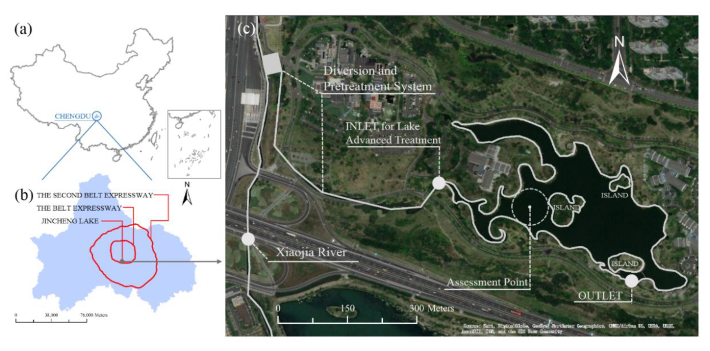
The Jincheng Lake is an artificial lake in the city of Chengdu, which is located in Southwestern China and has a subtropical monsoon humid climate (Figure 2). The annual average precipitation, temperature and wind speed here are about 1100 mm/year, 16 °C and 1.1 m/s, respectively.
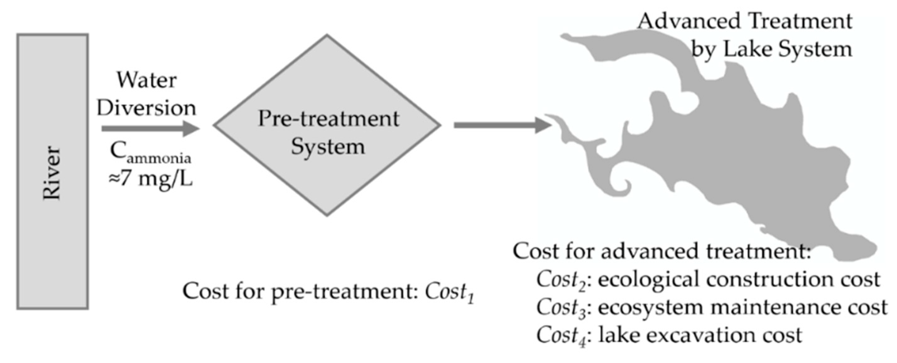
The integrated water treatment system at the Jincheng Lake is composed of a pre-treatment system and an advanced treatment system (the Jincheng Lake), as shown in Figure 3. The Xiaojia River, polluted by sewage, is the major recharge for the whole system. The polluted river water is diverted and firstly purified by the pre-treatment system consisting of a settling tank, a reaction pool, magnetic separation, and aeration. Then, the pre-treated water flows into the Jincheng Lake for the next advanced treatment, which is mainly accomplished by the self-purification capacity of the lake, further reducing contaminants in water.
The Jincheng Lake is still under construction, and the lake area was designed to be 11.3 × 10⁴ m2. The inlet is set in the west boundary, which pre-treated water is diverted in as the recharge of the lake, and the outlet is set in the southeastern part (Figure 2c). Rainfall-runoff generated around the Jincheng Lake is collected by municipal pipes. The artificial lake bed is covered by clay and an impermeable membrane to prevent seepage from the lake to groundwater, which is different from the natural water body closely connected with groundwater [31]. The decreasing rate of water level caused by evapotranspiration is approximately 1.1 cm/day according to the water level records in the Jincheng Lake during April and May in 2018. The midpoint of the southwestern lake was selected as the water quality assessment point by the management agency, as this open area is directly affected by the pre-treated water and can effectively reflect the self-purification capacity of the lake (Figure 2c). The ammonia concentration was chosen as the water quality indicator because ammonia is a critical nutrient of aquatic ecosystems that can lead to the death of animals, plants and plankton at a high concentration.

3.2. Numerical Model Calibration and Sensitivity Analysis

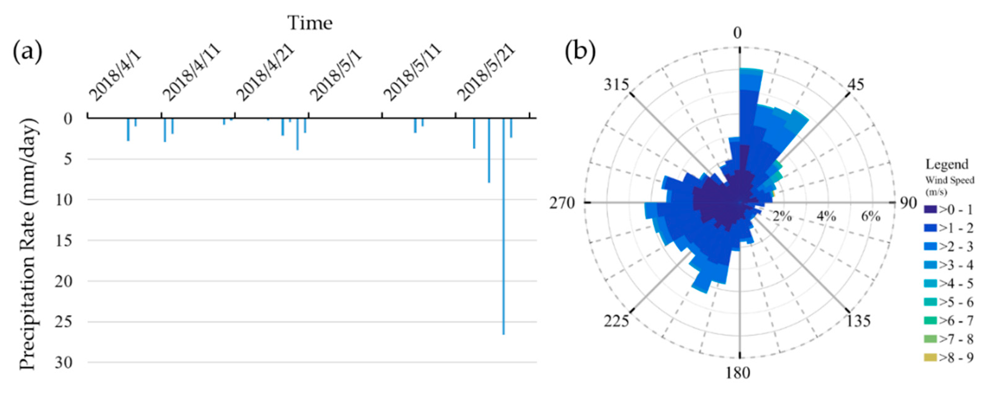
The simulation of hydrodynamic and water quality processes through MIKE21 needs various types of driving data. Elevation data were extracted from the blueprint, and the digital elevation mesh data were further generated by interpolating the discrete elevation data using the kriging method. Meteorological data were downloaded from the China National Meteorological Information Center (http://data.cma.cn/). Figure 4 shows the precipitation and wind data from 0:00:00 on 1st April, 2018 to 0:00:00 on 31st May, 2018 with a temporal resolution of 120 s. Water pressure data loggers (Schlumberger Water Services, Canada) were placed on the lake bed at the assessment point to measure the sum of barometric and water pressure (P1), and on the island to measure the barometric pressure (P2). Hence, water depths at the assessment point can be calculated from measured pressure data (described as: depth = P1/ρg − P2/ρg, where ρ and g are water density and gravitational acceleration, respectively). The resolution of pressure was 2.0 cm H2O with an accuracy of ±5.0 cm H2O. The temporal resolution was set to 10 min for these two loggers. Both observed water level and ammonia concentration data were collected at the assessment point during the simulation period. Water samples were collected every 3 days and the ammonia concentration was measured in the water quality analysis lab of POWERCHINA Chengdu Engineering Corporation Limited. The calibration of the numerical model was operated manually in a trial-and-error manner. The objective of this calibration was not to optimize the goodness-of-fit while it was to adequately regenerate the spatiotemporal patterns of the lake water table and ammonia concentrations.
In this study, four input variables were defined as determining parameters in optimization modeling: the water flow diverted from the upstream river into the pre-treatment system (Q, m3/s), the ammonia concentration after pre-treatment (C, mg/L), the designed water depth in the assessment point (D, m) and the biological respiration intensity (P, day−1) in MIKE21 (characterizing the designed density of animals and plants in the lake). These variables should have a significant sensitivity and engineering controllability, which means that they could be adjusted by engineering activities. To examine the magnitude of input data impacts on the model outputs, a sensitivity analysis was conducted for these four input variables (Q, C, D, and P). Because the calibrated current situation of construction period is absolutely different with the design of operation period, benchmarks of Q, C, D, and P were set as 0.03 m3/s, 2 mg/L, 1.95 m and 3 day−1, respectively. For the sensitivity analysis, each input varied ±50% on the basis of the base value to see the change of daily averaged ammonia concentration during the steady state, only one input was altered at a time and the other three were kept unchanged.

3.3. Surrogate Model Training

The surrogate models generated by the SVM and the ANN were trained and validated by the data collected from the numerical model. The training samples were generated by running the numerical model for specified times using different sets of input data. A MATLAB (Mathworks, Natick, MA, USA) program was developed to generate input files for MIKE21 and a script was prepared to invoke MIKE21 automatically. The numerical models were run in parallel at seven cloud servers (HUAWEI Cloud, https://www.huaweicloud.com/). The parameters of surrogate models were tuned and validated to maximize the coefficient of determination (R2). During the tuning of surrogate models, a total of 600 samples of training data were used while more than 400 samples were generated for the validation, which needed approximately 5 days for computation on seven cloud servers. The Latin Hypercube Sampling (LHS) [32] was applied to conduct the sampling scheme, enabling relatively better representativeness for the total samples with a limited size.
For surrogate models trained with ANNs, with more neurons used in the hidden layer, the response surface performs more accurately. However, it may lead to overfitting, with generation ability decreasing. Therefore, numerical experiments with different numbers of neurons and various data sizes were designed in our study. Since the initial weight values of ANN were randomly set at the beginning of the training, different ANN models were created for each training process, yielding varying performances. Hence, the evaluation of ANN performances in this study depends on the average R2 calculated by repeating the ANN model generation process 100 times.

3.4. Multi-Objective Optimization

In this study, the balance between the total cost and the water treatment ability of Jincheng Lake was concerned. A coupled simulation-optimization model was developed to explore the optimal design strategy for the Jincheng Lake with two main objectives: minimizing the expected engineering total costs in 10 years and the target pollutant concentration at the assessment point. The GA was used to catch the Pareto front. MATLAB solver “gamultiobj” was used to invoke the surrogate model and solve the optimization problem. The cost objective was formulated as follows:
Minimized Cost = Cost1(Q,C) + Cost2(P) + Cost3(P) + Cost4(D)
where Minimized Cost is the total quantified cost in the integrated system including the engineering construction cost (Cost2 + Cost4) and the operation cost (Cost1 + Cost3), Cost1 represents the expenses generated during the sewage treatment of the pre-treatment system, Cost2 is for building the lake ecosystem such as planting reeds, Cost3 indicates the expense for environmental maintenances like replanting vegetation, clearing silt and labor costs in the Jincheng Lake, and Cost4 is the expense spent on the lake excavation according to municipal planning. As a whole, Cost1 occurs in the pre-treatment system while Cost2, Cost3, and Cost4 take place in the lake construction and operation. These four terms were calculated as follows:
Cost1(Q,C) = Q × F1(C) × time
Cost2(P) = area × unitPriceEcoC × (P/P0)
Cost3(P) = area × F2(P) × time
Cost4(D) = unitPriceExcav × area × (DD0)
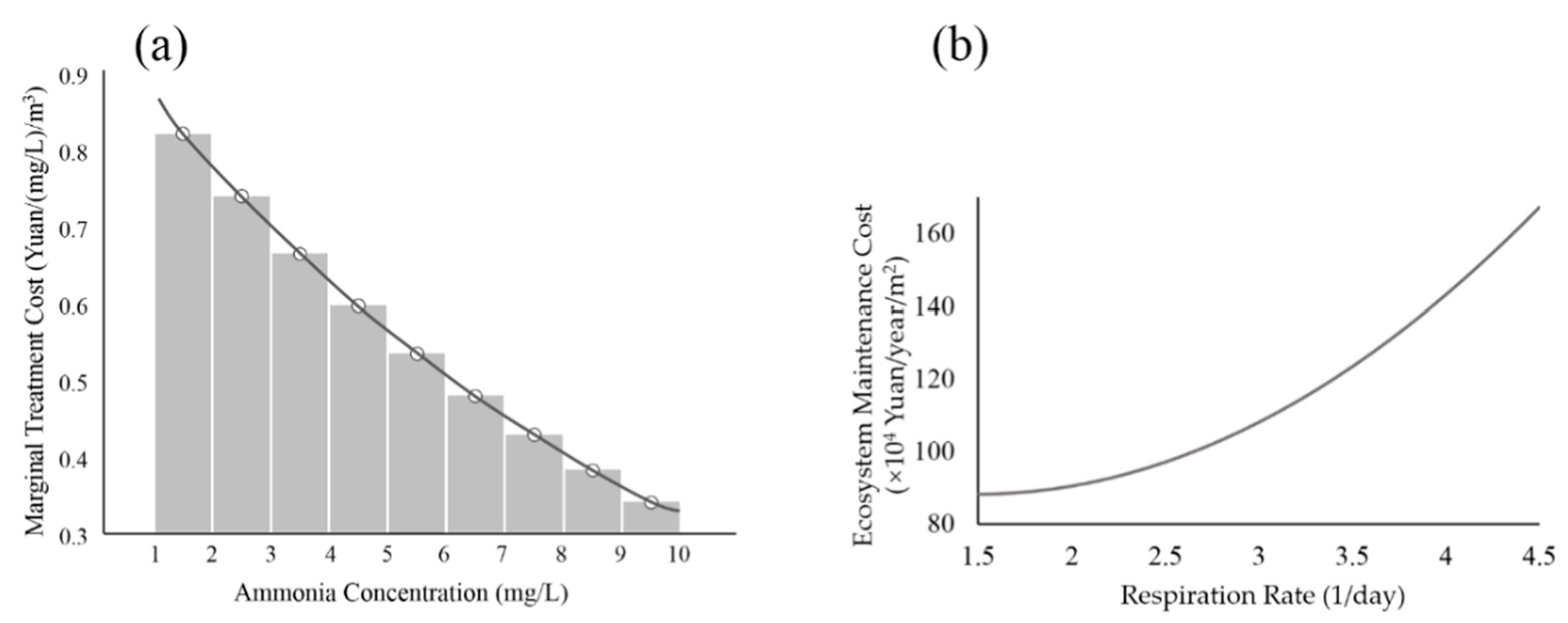
where parameters unitPriceEcoC (32.0 yuan/m2) in Cost2 and unitPriceExcav (10.7 yuan/m3) in Cost4 represent the unit prices of ecological construction and excavation costs, respectively; P0 and D0 are the maximum biomass and water depth under the present construction schemes; F2(P) is used to identify the maintenance cost reflected by P in the lake ecosystem. For water resources with different ammonia concentrations, Cost1 is obtained by the integral over the marginal cost curve of the pre-treatment system which is estimated based on the engineering cost database of traditional sewage treatment measures (Figure 5a). For instance, under the current condition (the ammonia concentration in the upstream is 7 mg/L), the unit cost of purification (F1(C)) to reduce the upstream ammonia concentration to midterm target concentrations (C) should be calculated as the integral of the marginal curve from 7 mg/L to C. This curve reflects that the unit cost of water treatments would rapidly increase with an improving water quality. The current common solution to solving this problem is to conduct advanced water purification by combining artificial lakes and wetlands with traditional sewage treatments.
As Figure 5b shows, when the respiration rate is beyond a certain value, the marginal ecosystem maintenance cost will increase rapidly with the rise of replanting and labor costs. It is noteworthy that the maintenance cost will not decrease even at a very low respiration rate. This is because the lake ecosystem with a lower density of species is easier to cause biological invasion, resulting in increasing costs to deal with it.
In summary, Q, C, P and D were defined as input variables. The relationship between input variables and total costs was calculated as above. The water treatment ability of the whole system characterized by the target pollutant concentration of the artificial lake was simulated by surrogate models based on these input variables.

4. Results and Discussion

4.1. Model Calibration and Sensitivity Analysis

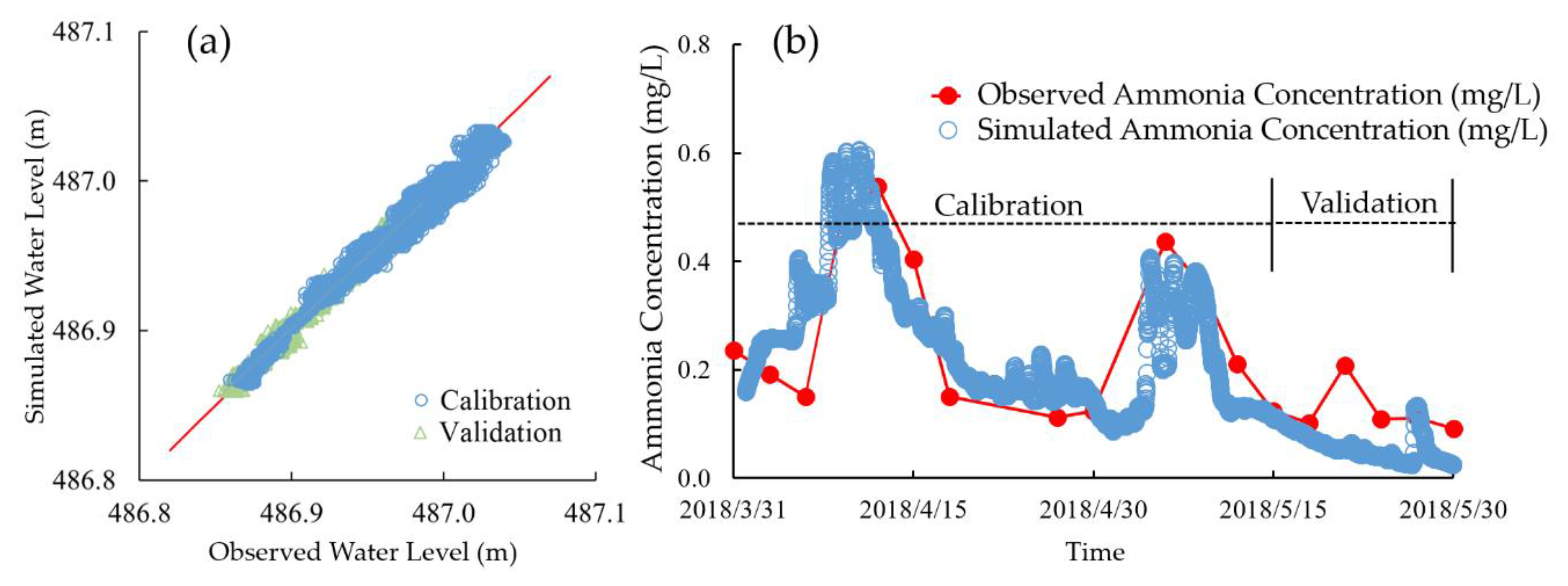
The comparison between simulated and observed water levels at the assessment point indicated a reasonable match with R2 of 0.981 in calibration and 0.977 in validation (Figure 6a). Meanwhile, the simulated ammonia concentrations also effectively exhibited the temporal variation of observed ammonia concentrations (Figure 6b). Both results revealed that the calibrated numerical model can properly interpret patterns of water levels and the water quality in this artificial lake. The setting of input data and calibrated parameters are presented in Table 1.
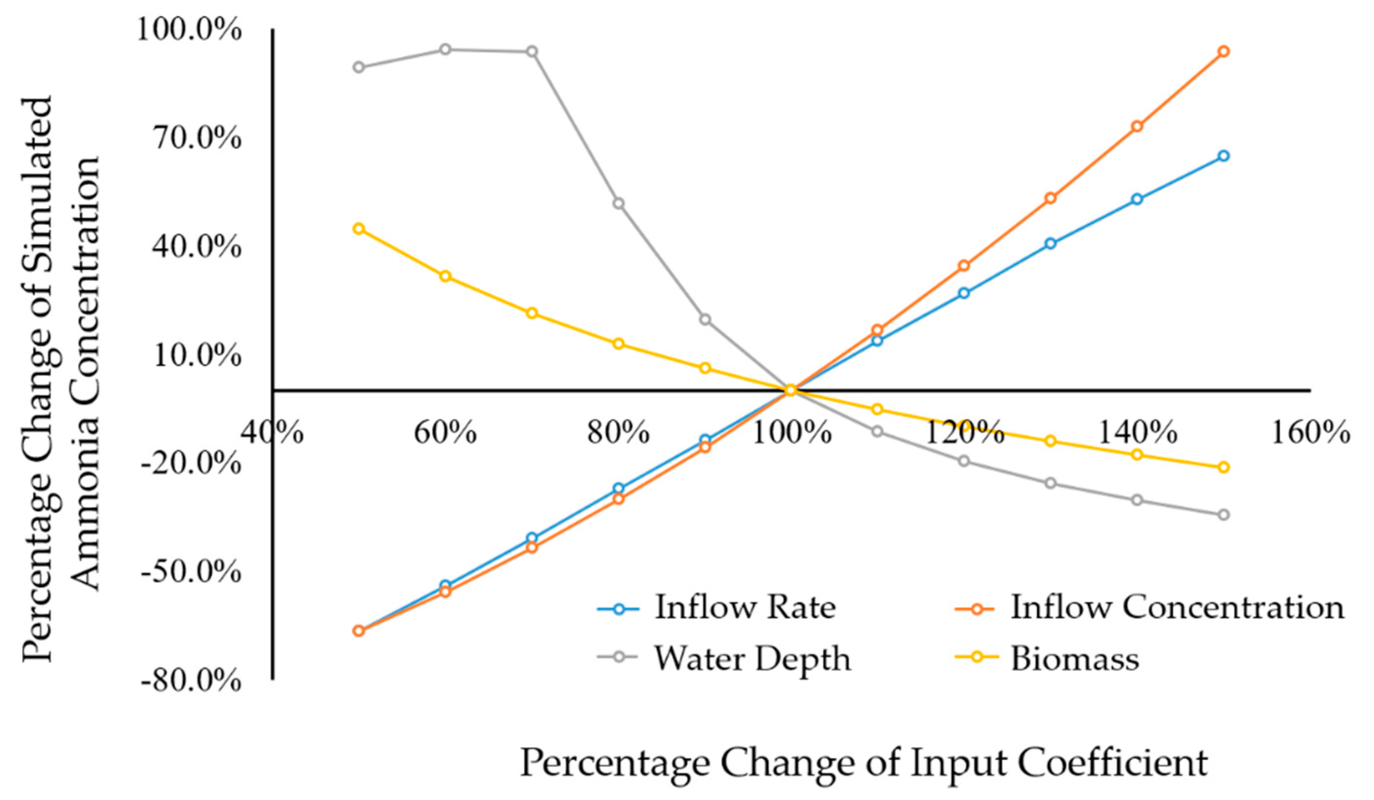
With input values varying ±50%, results of ammonia concentrations change in the ranges −66.7%–64.8% for Q, −66.7%–93.5% for C, 89.2%–−34.5% for D and 44.4%–−21.3% for P (Figure 7). Among these four variables, Q and C display evident positive correlations with the ammonia concentration, because the quantity and concentration of pollutants flowing into the lake are directly controlled by these two inputs. In contrast, the lake ammonia concentration decreases as D and P increase, indicating an improvement of the lake water quality accompanied by increased water environmental capacities and self-purification abilities. It should be noticed that the lake ammonia concentration will not continuously increase with decreasing water depth, because the absorption of pollutants by plants is suppressed at a very low level when the water depth is shallower than a certain value. In addition, much gentler slopes in D and P indicate that water depth and respiration rate have much less impact on the ammonia concentration than the inflow recharge rate and ammonia concentration. Overall, the remarkable impacts for all four input variables on the outputs further support the feasibility of subsequent surrogate model construction.

4.2. Surrogate Model Performances and Comparisons

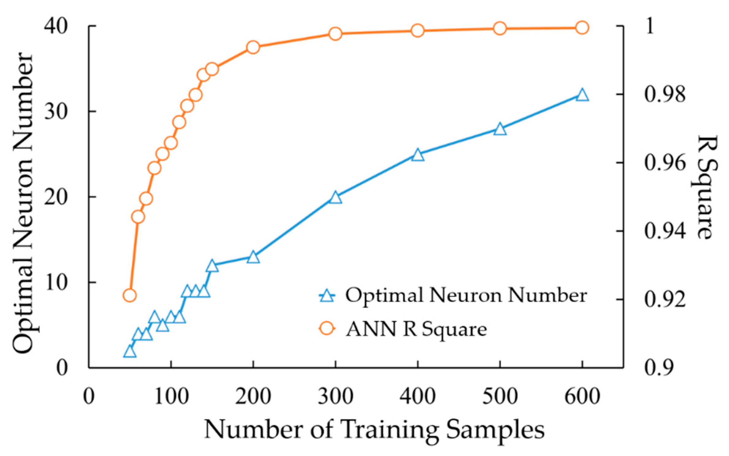
Performances of surrogate models by the ANN and the SVM were analyzed and compared with each other. For the ANN, a total of 544 surrogate models were built with 2 to 25 neurons in the hidden layer and the number of training data changing from 50 to 600. Results in Figure 8 demonstrate that for low-dimensional models like this study, with 4 inputs and only 1 output, the number of neurons which generates the optimum performance is changing with different sizes of training data. Generally, as the volume of training data increases, the optimal neuron number increases and the optimal network displays better performances. However, when the number of training samples exceeds 200 in this case, the optimal network does not significantly outperform the sub-optimal network, with the increasing risk of overfitting. The ANN has the linear time complexity (O(n)) and the SVM has the quadratic polynomial time complexity (O(n2)), where n represents the number of training samples. Both the ANN and the SVM has the linear space complexity (O(n))
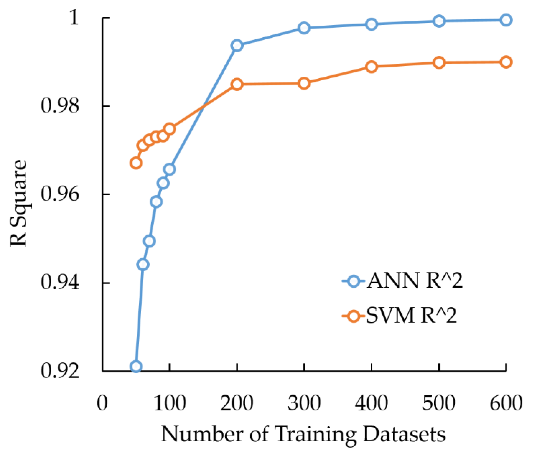
When 200 to 500 training samples are used, both the ANN and the SVM obtain good performances with R2 more than 0.98 (Figure 9). However, once the number of training datasets falls below 100, the training performance of ANN dramatically turns bad while SVM performs more steadily. The R2 of SVM can maintain over 0.95 using 50 to 100 sets of training data.
As reported in previous studies, response performances between ANN and SVM with different modeling dimensionalities and data sizes are different. As response surface surrogates of physically based numerical models, SVM has been reported having comparative performances as ANN in groundwater quality simulation (MT3D, nitrate), approximating the Soil and Water Assessment Tool (SWAT) model and computational fluid dynamics modeling [21,33,34]. These cases usually have smaller input data sizes at surrogates training steps compared with cases in this study. Furthermore, another kind of empirical model construction, which directly combines input and observed output data using learning machines to generate response relationships, gives close results. These black-box models generally have less modeling dimensions in rainfall-runoff modeling, river discharge prediction, water quality forecasting and related hydrological modeling fields [8,19,35]. In consequence, for this kind of low-dimensional (only one output and four input variables) water quality modeling projects, ANN should be preferred against SVM by a slim advantage of the fitting accuracy, in the premise of sufficient training data and time constraints.
The practical engineering is normally very time-sensitive, and computational analysis is the most time-consuming part in engineering designing. Hence, the comparison of the applicability of ANN and SVM utilized in engineering optimization has practical significance. For example, if the time for one model run is 30 min, the period of running the model for 100 times is about 2 days. With 100 sets of training data, SVM can generate acceptable results while the performance of ANN is not satisfying. On the other hand, ANN would be a better choice when about 300 sets of training data can be prepared within an ampler time (about 6 days). In the early design stage of an actual engineering project, SVM should be performed for the surrogate model construction with limited time (about 2–3 days) while ANN would be a better choice in a more relaxed time condition.

4.3. Multi-Objective Optimization of the Lake Design and Operation

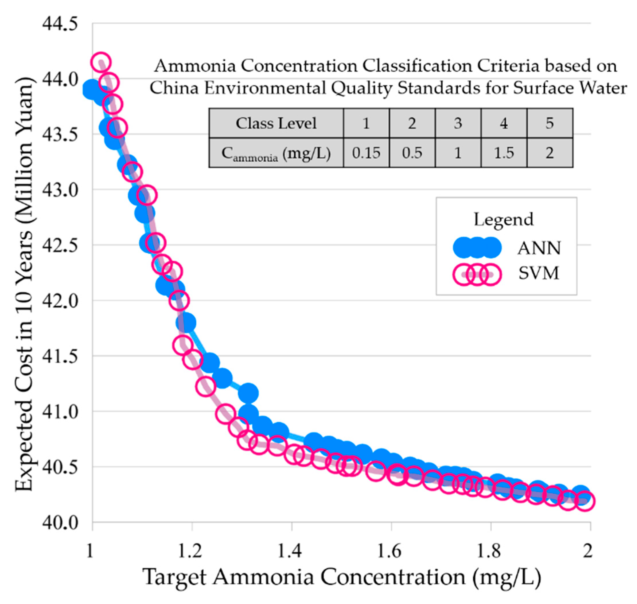
Under the current river pollution status (the ammonia concentration in the river is approximately 7 mg/L), the tradeoff between target ammonia concentrations at the assessment point and expected costs in 10 years is interpreted by the Pareto front (Figure 10). The slope of the curve reveals how much costs increase with a unit of target ammonia concentrations decreasing. The slope in low target ammonia concentrations is much higher than that in high target ammonia concentrations due to significantly increased construction and management costs. Hence, the turning point can be easily found at about 1.3 mg/L, indicating distinct kinds of economic efficiencies. For example, five water quality classifications from Class I to Class V with different uses have usually been used in traditional design for water treatment projects [36]. The criteria of ammonia concentrations in each class are shown in Figure 10. Classes III, IV and V were often set as treatment targets with ammonia concentrations being 1, 1.5 and 2 mg/L, respectively. The expected costs in 10 years were calculated as about 44.0, 40.5 and 40.2 million yuan using both ANN and SVM when the target was set as Classes III, IV and V, respectively. It means that only additional 0.3 million Chinese yuan needs to be spent in improving the water quality from Class V to Class IV. For water quality improvement from Class IV to Class III, a much higher cost with the value of 3.5 million Chinese yuan is needed. In addition, for more refined water quality management, the ammonia concentration target around 1.3 mg/L could be an optimal choice.
To provide scientific suggestions for future situations, a series of scenarios with the ammonia concentration of upstream river ranging from 4 to 10 mg/L were conducted. As expected, when the ammonia concentration of the upstream river increases, the Pareto front curve will move up, revealing that an upstream river water quality degradation results in larger costs under the same target ammonia concentration of lake water. On the other hand, the turning points of different scenario curves are all located at the concentration of about 1.3 mg/L, coinciding with the current situation. The result also demonstrates the validity of the optimal scheme even if the environmental background changes. With the target ammonia concentrations fixed at about 1.3 mg/L as discussed above, the simulated optimal expected costs increase by about 6 million yuan when ammonia concentrations of the upstream river increase by each 1 mg/L, ranging from 21.9 to 55.7 million yuan. Furthermore, as shown in optimal schemes in Table 2, the fractional costs of pre-treatment increase from 28% to 59% with ammonia concentrations of the upstream river varying from 4 to 10 mg/L, illustrating that the improvement of background environment would cut down relative costs of pre-treatments. When the environment around the lake has effectively improved, additional investments of the pre-treatment system will have less and eventually zero impact on lake water quality purification. Therefore, this study supports that more investments should be budgeted in the pre-treatment system operation instead of advanced treatments of the lake with deteriorated upstream river water qualities.

5. Conclusions

A new surrogate based approach was developed for an urban lake, the Jincheng Lake, to optimize the design and management strategies of artificial lakes. The core approach reconciles physically based numerical water quality models (like MIKE21 in this case) and surrogate models that make multi-objective optimization feasible and tractable in engineering projects. Machine learning approaches, specifically ANN and SVM, were used to train surrogate models for replacing complex numerical models. This greatly decreased computational costs of the proposed modeling-optimization paradigm, and obtained acceptable performance at the same time. The method we proposed offers scientific quantifications to make tradeoffs between engineering costs and water treatment.
The decision of setting the target criterion of ammonia concentrations of lake water as 1.3 mg/L was found optimal. With lower target pollutant concentrations (i.e., more strict criteria), expected total costs of the water treatment and ecosystem maintenance in 10 years rapidly rise, leading to an economically inefficient decision. In addition, considering further environmental background changes, multiple scenarios with different ammonia concentrations of the upstream river were set up and simulated. The simulation suggested that increasing upstream pollutant concentrations would lead to higher expected costs while the optimal ammonia concentrations in all scenarios were found unchanged at about 1.3 mg/L. Meanwhile, the allocations of total costs also exhibit higher ratios of water purification costs in the pre-treatment system with deteriorating water qualities of the upstream river. These results can offer specific and available guidance for the sustainable development of urban ecosystems under a changing environment.
Traditional approaches to optimization in water treatment industry are mainly based on experiences of designers. In traditional approaches, only a few examples would be settled and analyzed manually, which is obviously a rough method with limited ability to reach the real global optimal scheme. Compared with traditional measures of water environment planning and management, this mathematically based approach proposed in this study performs more scientifically and matches the tight schedule of engineering project at the same time. However, the approach proposed in this study faces challenge when dealing with high-dimensional surrogate modeling problems. More temporal and spatial assessment points will be needed for higher representativeness, leading to much higher dimensions of output features in surrogate modeling. For this kind of complicated surrogate model, more powerful training methods like deep learning should be developed.

Author Contributions

C.L. (Chuankun Liu), Y.H., T.Y., Q.X., and C.L. (Chaoqing Liu) conceived and designed the work plan; Y.H. and C.L. (Chuankun Liu) completed the modeling part; Y.H. and C.L. (Chuankun Liu) wrote the paper; C.S. and X.L. revised the manuscript. All authors have made contributions to this work.

Funding

This research was funded by the National Natural Science Foundation of China (NSFC, grant No.: 41807407).

Conflicts of Interest

The authors declare no conflicts of interest.

References

  1. Mortimer, C.H. Chemical Exchanges between Sediments and Water in the Great Lakes-speculations on Probable Regulatory Mechanisms. Limnol. Oceanogr. 1971, 16, 387–404. [Google Scholar] [CrossRef]
  2. Shutes, R.B.E. Artificial wetlands and water quality improvement. Environ. Int. 2001, 26, 441–447. [Google Scholar] [CrossRef]
  3. Moon, H.B.; Choi, M.; Yu, J.; Jung, R.H.; Choi, H.G. Contamination and potential sources of polybrominated diphenyl ethers (PBDEs) in water and sediment from the artificial Lake Shihwa, Korea. Chemosphere 2012, 88, 837–843. [Google Scholar] [CrossRef] [PubMed]
  4. Razavi, S.; Tolson, B.A.; Burn, D.H. Review of surrogate modeling in water resources. Water Resour. Res. 2012, 48, W07401. [Google Scholar] [CrossRef]
  5. Cai, X.; Zeng, R.; Kang, W.H.; Song, J.; Valocchi, A.J. Strategic planning for drought mitigation under climate change. J. Water Res. Plan. Manag. 2015, 141, 04015004. [Google Scholar] [CrossRef]
  6. Maier, H.R.; Kapelan, Z.; Kasprzyk, J.; Kollat, J.; Matott, L.S.; Cunha, M.C.; Marchi, A. Evolutionary algorithms and other metaheuristics in water resources: Current status, research challenges and future directions. Environ. Model. Softw. 2014, 62, 271–299. [Google Scholar] [CrossRef] [Green Version]
  7. Wang, C.; Duan, Q.; Gong, W.; Ye, A.; Di, Z.; Miao, C. An evaluation of adaptive surrogate modeling based optimization with two benchmark problems. Environ. Model. Softw. 2014, 60, 167–179. [Google Scholar] [CrossRef] [Green Version]
  8. Malekmohamadi, I.; Bazargan-Lari, M.R.; Kerachian, R.; Nikoo, M.R.; Fallahnia, M. Evaluating the efficacy of SVMs, BNs, ANNs and ANFIS in wave height prediction. Ocean Eng. 2011, 38, 487–497. [Google Scholar] [CrossRef]
  9. ASCE Task Committe. Artificial neural networks in hydrology. I: Preliminary concepts. J. Hydrol. Eng. 2000, 5, 115–123. [Google Scholar] [CrossRef]
  10. ASCE Task Committe. Artificial neural networks in hydrology. II: Hydrologic applications. J. Hydrol. Eng. 2000, 5, 124–137. [Google Scholar] [CrossRef]
  11. Ostad-Ali-Askari, K.; Shayannejad, M.; Ghorbanizadeh-Kharazi, H. Artificial neural network for modeling nitrate pollution of groundwater in marginal area of Zayandeh-rood River, Isfahan, Iran. KSCE J. Civ. Eng. 2017, 21, 134–140. [Google Scholar] [CrossRef]
  12. Sarkar, A.; Pandey, P. River water quality modelling using artificial neural network technique. Aquat. Procedia 2015, 4, 1070–1077. [Google Scholar] [CrossRef]
  13. Su, J.; Wang, X.; Zhao, S.; Chen, B.; Li, C.; Yang, Z. A structurally simplified hybrid model of genetic algorithm and support vector machine for prediction of chlorophyll a in reservoirs. Water 2015, 7, 1610–1627. [Google Scholar] [CrossRef]
  14. Gong, Y.; Wang, Z.; Xu, G.; Zhang, Z. A comparative study of groundwater level forecasting using data-driven models based on ensemble empirical mode decomposition. Water 2018, 10, 730. [Google Scholar] [CrossRef]
  15. Mohanty, S.; Jha, M.K.; Raul, S.; Panda, R.; Sudheer, K. Using artificial neural network approach for simultaneous forecasting of weekly groundwater levels at multiple sites. Water Resour. Manag. 2015, 29, 5521–5532. [Google Scholar] [CrossRef]
  16. Pan, C.C.; Chen, Y.W.; Chang, L.C.; Huang, C.W. Developing a Conjunctive Use Optimization Model for Allocating Surface and Subsurface Water in an Off-Stream Artificial Lake System. Water 2016, 8, 315. [Google Scholar] [CrossRef]
  17. Karahan, H.; Ayvaz, M.T. Simultaneous parameter identification of a heterogeneous aquifer system using artificial neural networks. Hydrogeol. J. 2008, 16, 817–827. [Google Scholar] [CrossRef]
  18. Cristianini, N.; Shawe-Taylor, J. An Introduction to Support Vector Machines; Cambridge University Press: Cambridge, UK, 2000. [Google Scholar]
  19. Liu, M.; Lu, J. Support vector machine—An alternative to artificial neuron network for water quality forecasting in an agricultural nonpoint source polluted river? Environ. Sci. Pollut. Res. 2014, 21, 11036–11053. [Google Scholar] [CrossRef] [PubMed]
  20. Lin, J.Y.; Cheng, C.T.; Chau, K.W. Using support vector machines for long-term discharge prediction. Hydrol. Sci. J. 2006, 51, 599–612. [Google Scholar] [CrossRef] [Green Version]
  21. Khalil, A.; Almasri, M.N.; McKee, M.; Kaluarachchi, J.J. Applicability of statistical learning algorithms in groundwater quality modeling. Water Resour. Res. 2005, 41, W05010. [Google Scholar] [CrossRef]
  22. Asefa, T.; Kemblowski, M.; Lall, U.; Urroz, G. Support vector machines for nonlinear state space reconstruction: Application to the Great Salt Lake time series. Water Resour. Res. 2005, 41, W12422. [Google Scholar] [CrossRef]
  23. Granata, F.; Gargano, R.; Marinis, G. Support vector regression for rainfall-runoff modeling in urban drainage: A comparison with the EPA’s storm water management model. Water 2016, 8, 69. [Google Scholar] [CrossRef]
  24. Tsoukalas, I.; Makropoulos, C. Multiobjective optimisation on a budget: Exploring surrogate modelling for robust multi-reservoir rules generation under hydrological uncertainty. Environ. Model. Softw. 2015, 69, 396–413. [Google Scholar] [CrossRef]
  25. Galán-Martín, Á.; Vaskan, P.; Antón, A.; Esteller, L.J.; Guillén-Gosálbez, G. Multi-objective optimization of rainfed and irrigated agricultural areas considering production and environmental criteria: A case study of wheat production in Spain. J. Clean. Prod. 2017, 140, 816–830. [Google Scholar] [CrossRef]
  26. Makropoulos, C.; Butler, D. A multi-objective evolutionary programming approach to the ‘object location’ spatial analysis and optimisation problem within the urban water management domain. Civ. Eng. Environ. Syst. 2005, 22, 85–101. [Google Scholar] [CrossRef]
  27. Brockhoff, D.; Zitzler, E. Objective reduction in evolutionary multiobjective optimization: Theory and applications. Evol. Comput. 2009, 17, 135–166. [Google Scholar] [CrossRef] [PubMed]
  28. Warren, I.; Bach, H.K. MIKE 21: A modelling system for estuaries, coastal waters and seas. Environ. Model. Softw. 1992, 7, 229–240. [Google Scholar] [CrossRef]
  29. Iturrarán-Viveros, U.; Parra, J.O. Artificial Neural Networks applied to estimate permeability, porosity and intrinsic attenuation using seismic attributes and well-log data. J. Appl. Geophys. 2014, 107, 45–54. [Google Scholar] [CrossRef]
  30. Shawe-Taylor, J.; Bartlett, P.L.; Williamson, R.C.; Anthony, M. Structural risk minimization over data-dependent hierarchies. IEEE Trans. Inf. Theory 1998, 44, 1926–1940. [Google Scholar] [CrossRef] [Green Version]
  31. Yao, Y.; Huang, X.; Liu, J.; Zheng, C.; He, X.; Liu, C. Spatiotemporal variation of river temperature as a predictor of groundwater/surface-water interactions in an arid watershed in China. Hydrogeol. J. 2015, 23, 999–1007. [Google Scholar] [CrossRef]
  32. Stein, M. Large sample properties of simulations using Latin hypercube sampling. Technometrics 1987, 29, 143–151. [Google Scholar] [CrossRef]
  33. Stephens, D.; Gorissen, D.; Crombecq, K.; Dhaene, T. Surrogate based sensitivity analysis of process equipment. Appl. Math. Model. 2011, 35, 1676–1687. [Google Scholar] [CrossRef] [Green Version]
  34. Zhang, X.; Srinivasan, R.; Van Liew, M. Approximating SWAT Model Using Artificial Neural Network and Support Vector Machine. J. Am. Water Resour. Assoc. 2009, 45, 460–474. [Google Scholar] [CrossRef] [Green Version]
  35. Behzad, M.; Asghari, K.; Eazi, M.; Palhang, M. Generalization performance of support vector machines and neural networks in runoff modeling. Expert Syst. Appl. 2009, 36, 7624–7629. [Google Scholar] [CrossRef]
  36. China EPA. Environmental Quality Standards for Surface Water; National Environmental Protection Agency of China: Beijing, China, 2002. (In Chinese)
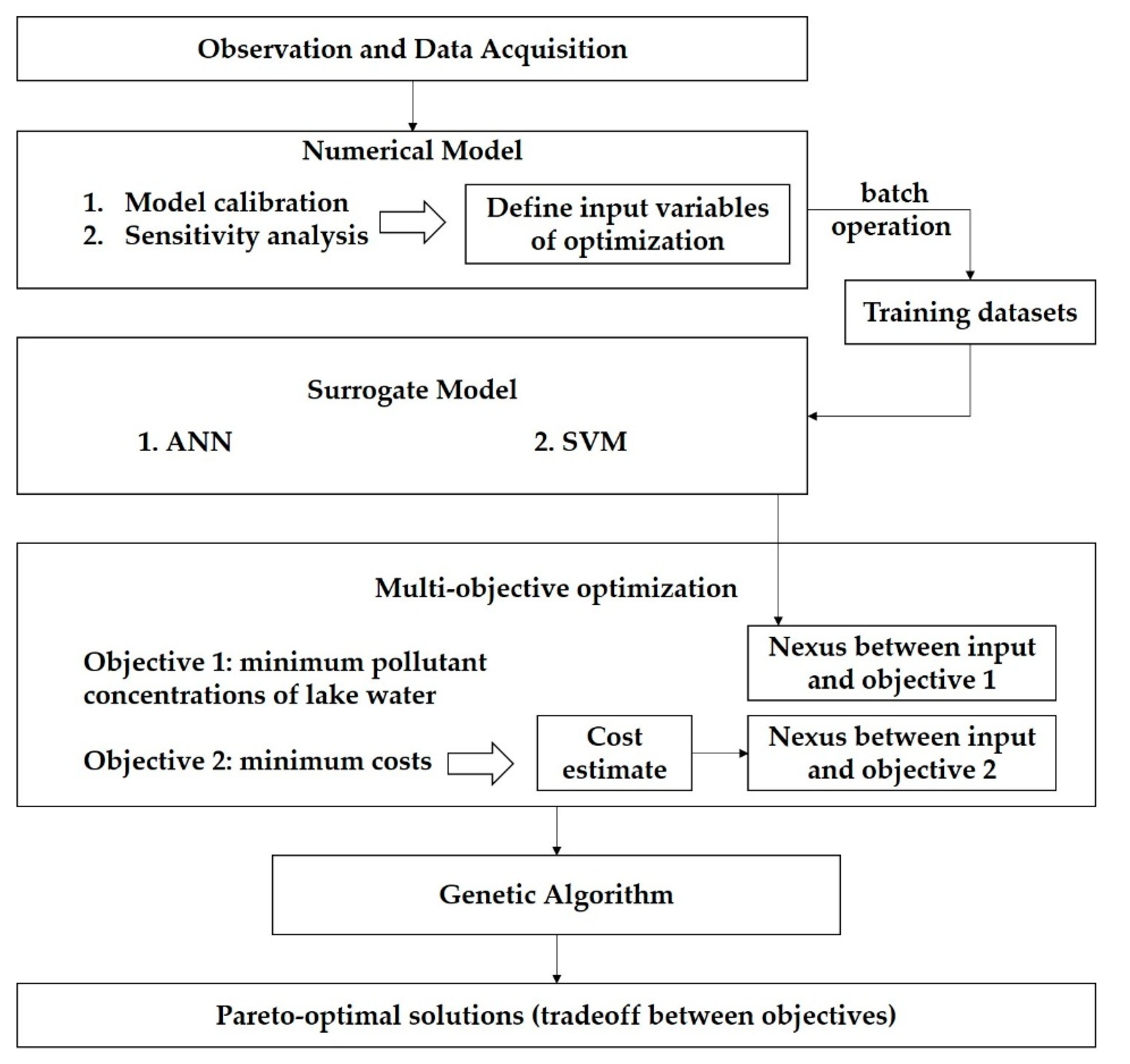
Figure 1. The modeling roadmap integrating a numerical model, surrogate models, and multi-objective optimization.
Water 11 00391 g001
Figure 2. Locations of (a) Chengdu City in China and (b) the Jincheng Lake in Chengdu, and (c) the satellite image of the integrated water system at the Jincheng Lake.
Water 11 00391 g002
Figure 3. The flow chart of the integrated water treatment system at the Jincheng Park, including the upstream river, a pre-treatment system and an advanced treatment system (the lake).
Water 11 00391 g003
Figure 4. The distribution of precipitation (a), wind speeds and directions (b) of the Jincheng Lake during the observing period.
Water 11 00391 g004
Figure 5. The marginal cost curves of the pre-treatment cost as a function of ammonia concentrations (a), and the ecosystem maintenance cost as a function of respiration rates (b).
Water 11 00391 g005
Figure 6. The model calibration and validation results of water levels (a) and ammonia concentrations (b) of lake water at the assessment point in the Jincheng Lake.
Water 11 00391 g006
Figure 7. Sensitivity analysis of the numerical model of the Jincheng Lake.
Water 11 00391 g007
Figure 8. The variations of the optimal neuron number in the hidden layer and R2 value of training performances as a function of the number of training samples changes.
Water 11 00391 g008
Figure 9. The comparison of surrogate model performances between ANN and SVM with the number of training datasets varying.
Water 11 00391 g009
Figure 10. The Pareto front of target ammonia concentrations vs. expected costs in 10 years using ANN and SVM, respectively.
Water 11 00391 g010
Table 1. Model parameters for the MIKE21 numerical model.
ItemValueUnitItemValueUnit
No. of time steps43200-Ammonia decay rate at 20 °C0.5day−1
Time step interval120sRecharge rate0.033m3/s
Simulation start date2018/4/1 0:00:00-Recharge ammonia concentration0.58mg/L
Simulation end date2018/5/31 0:00:00-Water depth at the assessment point1.95m
Smagorinsky eddy viscosity0.28-Respiration rate of animals and plants0.5day−1
Manning coefficient32m1/3/sMax. oxygen production by photosynthesis0.7day−1
The ration of ammonia released at BOD decay0.29gNH4/gBODUptake of ammonia in bacteria0.02-
Uptake of ammonia in plants0.03-
Table 2. The optimal target ammonia concentration of the lake and fractional costs of the pre-treatment system based on different ammonia concentrations of upstream river water.
The Ammonia Concentration of Upstream River Water (mg/L)The Optimal Target Ammonia Concentration (million yuan)The Fractional Costs of the Pre-Treatment SystemThe Ammonia Concentration of Upstream River Water (mg/L)The Optimal Target Ammonia Concentration (million yuan)The Fractional Costs of the Pre-Treatment System
421.928%846.554%
528.839%951.457%
635.245%1055.759%
741.250%