Modelling Snowmelt in Ungauged Catchments

1
Institute for Hydrology and Water Management (HyWa), University of Natural Resources and Life Sciences, 1190 Vienna, Austria
2
Department of Civil Engineering, University of Bristol, Bristol BS8 1TR, UK
Water 2019, 11(2), 301; https://doi.org/10.3390/w11020301
Submission received: 20 December 2018
/
Revised: 23 January 2019
/
Accepted: 29 January 2019
/
Published: 11 February 2019
(This article belongs to the Special Issue Study for Ungauged Catchments—Data, Models and Uncertainties)
Abstract
:Temperature-based snowmelt models are simple to implement and tend to give good results in gauged basins. The situation is, however, different in ungauged basins, as the lack of discharge data precludes the calibration of the snowmelt parameters. The main objective of this study was therefore to assess alternative approaches. This study compares the performance of two temperature-based snowmelt models (with and without an additional radiation term) and two energy-balance models with different data requirements in 312 catchments in the US. It considers the impact of: (i) the meteorological forcing, by using two gridded datasets (Livneh and MERRA-2), (ii) different approaches for calibrating the snowmelt parameters (an a priori approach and one based on Snow Data Assimilation System (SNODAS), a remote sensing-based product) and (iii) the parameterization and structure of the hydrological model used for transforming the snowmelt signal into streamflow at the basin outlet. The results show that energy-balance-based approaches achieve the best results, closely followed by the temperature-based model including a radiation term and calibrated with SNODAS data. It is also seen that data availability and quality influence the ranking of the snowmelt models.
1. Introduction
Snow has a hydrological impact beyond the areas on which it accumulates as it can dominate the river regime hundreds of kilometers downstream of snow-covered areas [1]. The importance of snow-related processes can be grasped when considering that in the year 2000 about 1/6 of the world’s population was estimated to live in areas where most of the discharge was snow-derived [2]. This indicates that enhancing our abilities for modelling snow accumulation and melt can result in widespread benefits.
Snowmelt modelling is important in mountainous areas, which are characterized by a lower density of measurement stations in comparison to more densely populated valley areas [1]. This explains why there are often no observed data available for setting up and validating hydrological models. The lack of climate data can be tackled by resorting to gridded climate datasets, which provide interpolated values onto a grid. These datasets might, however, have large uncertainties, especially in mountainous areas, where the complex topography and large elevation gradients constitute an additional challenge for interpolating climate variables [3]. Nevertheless, as temperature data provided by gridded datasets tend to have a good quality, they still can be a useful data source for temperature-based snow models [3]. These models rely on parameters relating air temperature to the phase of precipitation and the snowmelt rate. Ideally, the parameters would be estimated a priori based on the catchment properties. However, as it has not yet been possible to identify relationships between the catchment properties and the parameter values (e.g., [4,5,6]), they need to be calibrated [4,7]. While this can be best done with snow measurements (e.g., snow depth or snow water equivalents), it is also possible to use discharge data. In fact, this is the approach for calibrating snow parameters adopted by many operational hydrological models due to the scarcity of direct snow measurements. As ungauged basins lack discharge data, it is necessary to resort to other sources of snow-related information that can aid in the estimation of snow parameters. A viable option is using remote sensing imagery [8,9], which is expected to become more important as the coverage and resolution of remote sensing data increases and as better techniques for extracting useful information from them are developed.
Another approach for modelling snowmelt in ungauged catchments is to use physically based models as they do not require calibration. On the other hand, they are more complex and tend to have higher data requirements than temperature-based models. This is, however, not always the case as there are multiple ways of describing and parameterizing the terms of the energy-balance equation, which results in some degree of flexibility for adjusting to the available data. An extreme example is an energy-balance model that only uses the minimum and maximum daily temperatures as inputs [10].
This study was motivated by the need for a reliable approach for modelling snowmelt in ungauged basins. While previous studies have reported a similar performance for temperature and physically based models in gauged basins [4,11,12], their relative performances have not been assessed in ungauged catchments. It is, however, reasonable to expect that energy-balance models will have a better performance than temperature-based models as the latter will run with uncalibrated parameters. On the other hand, it is possible that the parameters of the temperature-based models can be successfully calibrated with the help of remote sensing data in which case there might be only small differences between energy and temperature-based snowmelt models. The main objective of this study is to compare different snowmelt approaches that can be applied in ungauged basins and to identify which of them should be used. The study considers the impact of: (i) using different forcing datasets, (ii) calibrating the snowmelt parameters with different approaches and (iii) the complexity of the hydrological model. For obtaining more representative results, the study is carried out for 312 catchments in the US.
2. Modelling Snow Accumulation and Melt
This section reviews with some detail the alternatives for modelling snow accumulation and snowmelt using temperature-based models. It emphasizes the values and ranges of the parameters describing these processes as it is later necessary to define a priori values for these parameters. A brief overview of the used energy-balance snowmelt models is presented for completeness.
2.1. Snow Accumulation
Although there are many factors influencing the precipitation phase, such as humidity and air pressure [13,14], only the near-surface air temperature tends to be used for modelling snow accumulation in hydrological models. In these cases, the precipitation phase can be estimated with a single temperature threshold or a linear or S-shaped curve transition between two threshold temperatures [14]. Numerous studies have been carried out for defining these thresholds. An analysis of 502 SNOTEL (SNOwpack TELemetry) stations, for instance, found that a threshold of 0 °C underestimated snowfall [14], as shown by a bias of −7%. Another study involving 15,000 land stations found that almost 95% of the precipitation falls as snow at −2 °C. This decreases to about 80%, 20% and 0% of snow at temperatures of 0 °C, 2 °C and 6.5 °C, respectively [13]. This agrees well with a literature survey recommending a rain/snow threshold of 1.7 °C considering that 97% of precipitation fell as snow below −0.5 °C and that 81% of the precipitation was rainfall when temperature was above 2.8 °C [5]. This is also consistent with studies in mountainous areas, which observed that about 90% of the precipitation was solid at 0 °C [15].
It was also observed that most precipitation events produce either rain or snowfall and that mixtures between both phases were rather uncommon [13]. It might be thus advisable to use a single threshold or to assign a single phase to all precipitation based on the probability of occurrence of each phase when considering two thresholds.
Since there is not much available data for validating more complex approaches, this study models snow accumulation as a function of a single threshold, . Incoming precipitation is assumed to be in a liquid state when the air temperature is above the threshold; otherwise, it is regarded as snowfall.
2.2. Snowmelt
The methods for modelling snowmelt are usually classified as either temperature-index [4,16] or energy-balance approaches. This study uses two temperature-based and two energy-balance snowmelt models which are described in the next sections.
2.2.1. Classic Temperature-Based Approaches (Tb)
Temperature-index approaches take advantage of the high correlation between temperature and snowmelt [4,17] and the relatively easy access to temperature data. Snowmelt (M in mm·day−1), is proportional to the difference between air temperature ( in °C) and a base temperature ( in °C). The air temperature can be defined either as the average or maximum daily temperature [5]. The factor of proportionality ( in mm·°C−1·day−1) is called melt or day-degree factor [4]:
The melt factor depends on the importance of individual components of the energy budget equation [4,18]. A higher fraction of shortwave radiation (found at higher elevations) is linked to higher day-degree factors. On the contrary, locations with high sensible heat fluxes tend to have lower day-degree factors. Sublimation, which might consume high amounts of energy, explains the lower day-degree factors that can be found in dry locations with high radiation. As the importance of different energy-balance components varies across seasons, it can be expected that this will be reflected in a seasonal variability of the day-degree factors. While this could be identified at plot scale studies, this is not necessarily the case at the catchment scale. A study involving 380 catchments showed, for instance, that a seasonally varying day-degree factor did not result in significant increases in model performance [19].
It is important to mention that some temperature-based snowmelt approaches might consider additional processes (e.g., refreezing, cold content). As their inclusion does not lead to important or consistent performance improvements at the catchment scale [19,20], they are not considered in the present study.
In general, it is considered that the day-degree approach is only valid for “average” conditions [18]. From a spatial point of view, it means the approach is not suitable for small areas, as the heat balance equation could be strongly affected by local characteristics. From a temporal point of view, it means that it is not suitable for sub-daily scales, but that it should be implemented for timescales covering the variability of “typical” weather and when conditions are close to average.
Regarding the parameter values, several reviews and studies have found that the day-degree factor tends to vary between 2.7 and 12 mm·°C−1·day−1 (e.g., between 3.5 and 6 mm·°C−1·day−1 [21]; 2.7 mm·°C−1·day−1 for a watershed in Alaska [22]; 2.7 and 11.6 mm·°C−1·day−1 with a median of 4.5 to 5 mm·°C−1·day−1 [4]). The authors of a study reviewed the parameter ranges used in recent simulation studies and then decided to consider a variation range between 0 and 20 mm·°C−1·day−1 [23]. The base temperature is often assumed to be 0 °C [24], but also varies across studies (e.g., from −2 °C to 5.5 °C in a study considering 24 basins [6]).
2.2.2. Temperature-Based Approaches with Radiation (Enhanced Temperature-Based Approaches) (TR)
These models attempt to benefit from the good results obtained with the simple temperature-index approaches and to address one of their main drawbacks by making them more physically based through the inclusion of radiation data [21]. One difference between applications is the considered radiation component, since some approaches use the total net radiation [21,25,26], while others consider the net shortwave radiation [22,27,28] or the incoming clear-sky shortwave radiation [29]. Another difference is that some models use measured radiation data as input, while others parameterize the radiation terms. As the incoming solar radiation shows consistent patterns with topography (e.g., slope, aspect), time of the year (e.g., sun declination) and location (latitude, elevation), there are some interesting approaches for getting distributed inputs that do not require additional climate observations [29,30,31]. This indicates that these combined approaches might not necessarily require more input data than temperature-index models [27]. This study implements the model described in Kustas et al. [21]:
with R representing the total net radiation (W·m−2) obtained from the input datasets. The parameter is a factor for converting the energy flux density to snowmelt depth. It is about 0.026 cm·day−1·(W·m−2)−1 and can be easily derived from the specific latent heat of water (334 kJ·kg−1). With respect to the melt factor, it is expected that it will be smaller than the one in the classical day-degree approach, since the radiation term already accounts for part of the melt. There is, however, not much information about the ranges of this factor, which is partly explained by the fact that its value will depend on the considered radiation terms. When using the shortwave radiation it was found that a value of about 2 to 2.5 mm·°C−1·day−1 provided good results for a Swiss catchment [26], while a melt factor of 2.3 mm·°C−1·day−1 was obtained for a watershed in Alaska [22]. Using the total net radiation a value of 5 mm·°C−1·day−1 was observed in a catchment in Vermont [25] and a value of 1.8 mm·°C−1·day−1 was obtained at a site in Switzerland [21].
2.2.3. Classic Energy and Mass Balance Approach (Eb)
While there are complex snow physics models providing information about the macroscopic (e.g., density, water content) and microscopic (e.g., ice grain size and shape) properties of various snow layers [32] most snow energy-balance models focus only on the energy balance in the snowpack. This can be represented by:
where U (kJ·m−2) stands for the energy. The terms in the energy balance are: (net shortwave radiation); (net longwave radiation), (advected heat from precipitation), (ground heat flux), (sensible heat flux) and (latent heat flux). The sign convention used here defines (i) all radiation fluxes as being positive when they are directed to the surface and (ii) the remaining energy fluxes (latent and sensible heat) as positive when directed away from the surface [33]. With respect to the relative importance of the energy-balance terms, and account usually for 60–90%, and for 5–40%, for 2–5% and for 0–1% of it [24]. The low impact of the last two terms explains why they are often neglected. Most of the approaches and equations adopted in this study are taken from Tarboton et al. [34], where more detailed information can be found.
The net solar radiation and longwave radiation were obtained directly from the input datasets. The turbulent fluxes of sensible and latent heat between the snow surface and the air above are proportional to the difference in temperature and vapor pressure, respectively. The proportionality constants are known as turbulent transfer coefficients or diffusivities:
with and (dimensionless) being the transfer coefficients, k is the dimensionless von Karman constant, z is the height at which the wind velocity is measured (m) and is the roughness height (m).
The sensible and latent heat fluxes are then calculated as:
where is the air density (kg·m−3) estimated with the atmospheric pressure derived from the elevation using the barometric formula and the air temperature ( in K). is the specific air capacity (1.005 kJ·kg−1·°C−1) and u is the wind speed (m·day−1), is the dry gas constant (287 J·kg−1·K−1) and is the latent heat of sublimation (2834 kJ·kg−1). is the air vapor pressure and the vapor pressure at the snow surface which is assumed saturated at the temperature . Many authors consider stability correction factors for the turbulent fluxes based on the Richardson number [22,35]. However, as some studies found that they might lead to unreasonable values [34,36,37], they are not included here. Since and are neglected, the surface temperature is obtained by minimizing the absolute sum of the four remaining terms in the energy-balance equation. This temperature is then used for estimating the energy available for snowmelt and the snowmelt (mm) is obtained with:
with being the heat of fusion (334 kJ·kg−1) and the density of water (kg·m−3).
2.2.4. Energy and Mass Balance Approach with Reduced Input Data Requirements (Wa)
This model was first presented by Walter et al. [10] and requires only the timeseries of the daily precipitation and temperature extremes. The equations are similar to the ones presented in the previous section. They are described in detail in Walter et al. [10] and were also implemented in an R package [38]. For the terms that had a different parameterization in both sources, the most recent was adopted (i.e., the one from the R package [38]). The incoming radiation S (kJ·m−2·day−1) is estimated as a function of the albedo A (dimensionless), the atmospheric transmissivity (dimensionless) and the potential extraterrestrial solar radiation (kJ·m−2·day−1):
The albedo ranges between 0.25 (ground albedo when there is no snow) to a value close to 1 assigned to new snow. A simple decay function is used for modelling the decrease in albedo of snow in time. The transmissivity is estimated using the approach outlined in Bristow and Campbell [39]:
with B being an empirical coefficient depending on the difference between the daily minimum and maximum temperatures . The extraterrestrial solar radiation is estimated as a function of the latitude (radians) and the solar declination angle (radians) estimated according to Rosenberg [40]:
with J being the day of the year. The terrestrial longwave radiation (kJ·m−2·day−1) is estimated with the Stefan-Boltzmann equation:
with being the surface emissivity (dimensionless) estimated with the daily temperature and the fraction of cloud cover obtained as a function of the transmissivity; is the Stefan-Boltzmann constant and the temperature T (in K). The sensible and latent heat fluxes are estimated with the same equations shown above for the classic energy-balance approach. Instead of the daily wind speed the approach presented here relies either on the long-term average at the respective location or on the geometric mean value of the nearest catchments with wind data. The vapor density was approximated as the saturation density at the minimum daily air temperature. For the ground heat flux a constant value of 173 kJ·m−2·day−1 was assumed, and the advected heat from precipitation was estimated with:
With being the heat capacity of water (in kJ·m−3·°C−1); P the rain depth (m) and the air temperature (°C).
3. Materials and Methods
3.1. Study Areas
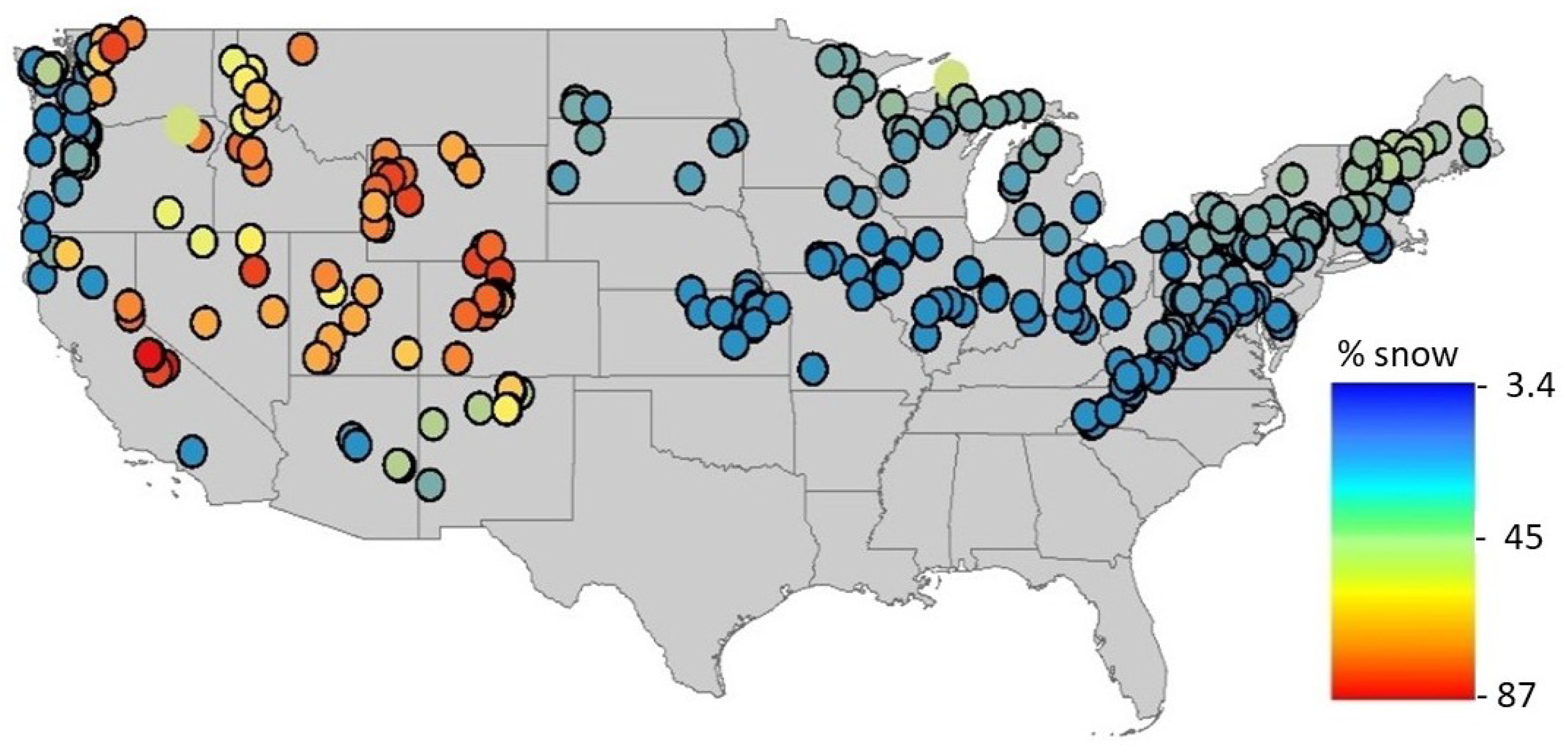
This study was carried out for a set of 312 GAGES II (Geospatial Attributes of Gages for Evaluating Streamflow, version II) reference basins (Figure 1, Table 1). The catchments were selected based on the presence of snow (fraction of snow in the total precipitation >2%) and in the performance of the hydrological model. The intention behind filtering the catchments according to the achieved performance was to remove from the analysis the catchments that could not be well modelled. The study considers therefore only the catchments that achieved a Nash–Sutcliffe coefficient larger than 0.4 in a previous study based on 574 GAGES II catchments using the same hydrological models considered here, albeit for a different period and calibration approach. It might be further important to be aware that snow constitutes a seasonal feature in most catchments, but that 22 of them have areas permanently covered with ice or snow.
3.2. Datasets
This section presents the data used in this study: two datasets used as model forcings (Livneh and MERRA-2), one dataset used as calibration target for the snow parameters (SNODAS) and the discharge data (from the United States Geological Survey, USGS) used as calibration target for the rainfall-runoff model.
3.2.1. Livneh Dataset
The Livneh dataset [42] is an updated version of the Maurer dataset [43]. It provides daily precipitation, temperature (minimum and maximum) and wind velocity data for the conterminous US between the years 1915 and 2011. The data lies on a 1/16 degrees grid and has a temporal resolution of 3 h. Data for following variables was downloaded for this study: total precipitation rate (mm), near-surface (2 m) air temperature (K), near-surface (10 m) wind speed (m·s−1), near-surface (2 m) relative humidity (%), downward solar radiation (W·m−2), net solar radiation (W·m−2), downward longwave radiation (W·m−2) and net longwave radiation (W·m−2).
3.2.2. MERRRA-2 Dataset
The first version of the MERRA dataset aimed at modelling the atmospheric water balance [44]. An updated version (MERRA-2) was produced for addressing some weaknesses of the original product and for updating the input data sources [45]. The grid has a spatial resolution of 0.625 × 0.5 degrees and was downloaded for each hour. The variables used in this study were: the specific humidity at 2 m (kg·kg−1), the air temperature at 2 m (K), the net longwave and shortwave radiation (W·m−2), the total bias corrected precipitation over land (kg·m−2·s−1) and the surface wind speed (m·s−1). As the spatial resolution of the climate data has a large influence on the snow processes it was decided to downscale the MERRA-2 data to the Livneh grid using monthly temperature, precipitation, and relative humidity correction factors. The monthly value of each variable in the Livneh grid was obtained from the ClimateNA tool [46]. The relationship between the mean value of the corresponding variable for the entire MERRA-2 cell and each of the smaller Livneh grid cells contained in it, was then used for estimating the value of each cell in the Livneh grid. Further information about this procedure can be found in the Supplementary Materials.
3.2.3. SNODAS Dataset
The SNODAS (SNow Data Assimilation System) dataset [47,48] provides estimates about the snow cover and associated snow variables in a 1km grid. It combines data from a weather model, a physically based spatially distributed snow model and observations of the snow-covered area and snow water equivalents (from satellites, airborne equipment, and ground stations). It is produced by the NOAA National Weather Service National Operational Hydrologic Remote Sensing Center (NOHRSC) and covers the conterminous US at a daily timestep from September 2003 to the present. One aspect that needs to be considered when using this dataset is that its quality has not been thoroughly assessed, as all data at a 1 km scale that could be used for validation are already used as model input [47]. Some studies have evaluated the quality of some SNODAS variables, mainly the SWE and snow depth, using field measurements [49,50]. This is, however, a highly resource intensive approach which provides information for only a small area. Other studies compared SNODAS variables with the results from other airborne and satellite derived data [50,51] or carried out evaluations at the basin scale using discharge measurements [49,52]. The outcomes of these experiments are variable and do not allow an overall estimate of the quality of the dataset.
3.2.4. Discharge Data
This study aims at comparing the performance of different snowmelt models. This would be ideally done by comparing the output of the snow models directly to snowmelt data, for instance, the SNOTEL data which is collected by the NRCS (US Natural Resources Conservation Service). Since there are, however, only a few stations delivering all forcing data required by the hydrological models, it would have been necessary to use gridded forcing data for estimating snowmelt at the point scale (i.e., the SNOTEL station). Since the value of climate variables at a specific point might not correlate well with the value of the gridded cell, this study uses discharge data for evaluating the snow models. An advantage of this approach is that the spatial scales of the input data (gridded input) and the output variables (basin discharge) have a better match, as both describe aereal averages. Another positive aspect it that it allows to consider a large number of catchments, instead of only a few SNOTEL stations.
The daily discharge data between the 1 January 1980 and the 31 December 1980 was downloaded from the USGS webpage. No additional checks on this data were carried out, as the USGS data undergoes detailed QM/QA (quality management/quality assurance) procedures (see chapter 502.2 of the USGS Survey Manual: Fundamental Science Practices: Planning and Conducting Data Collection and Research).
3.3. Snowmelt and Hydrological Models
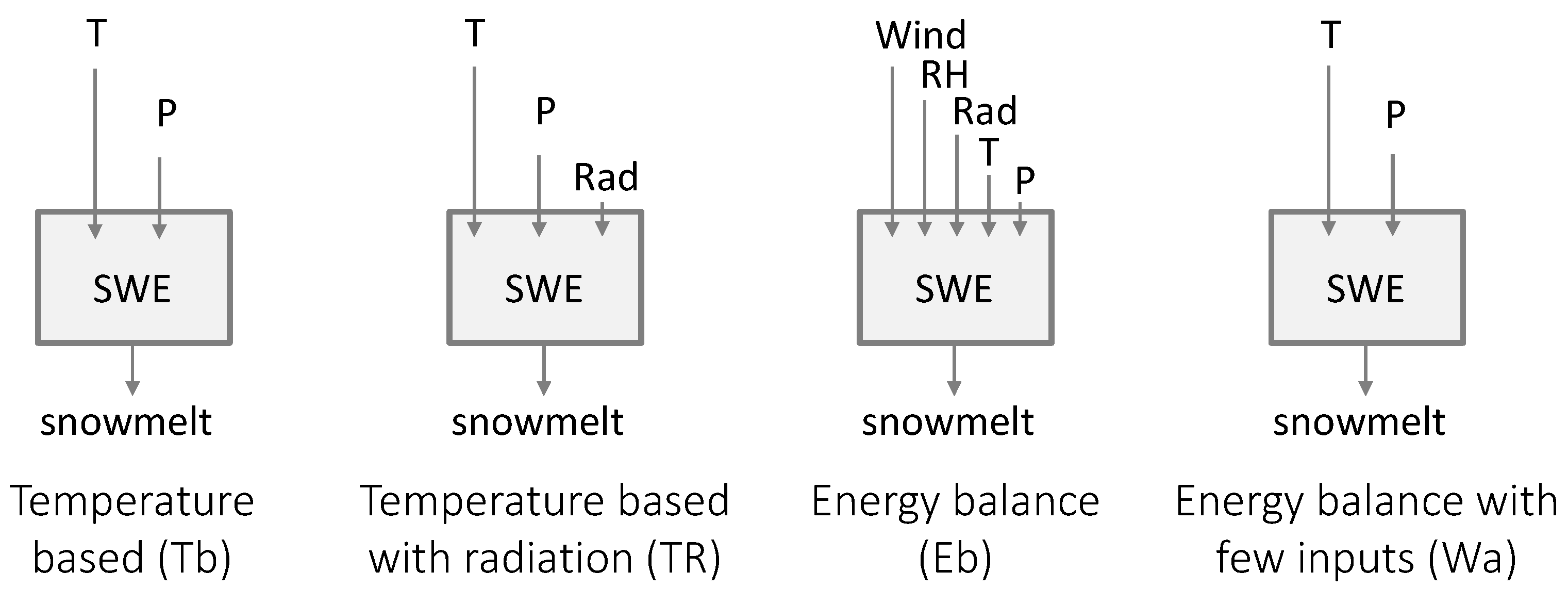
This study assesses the performance of different snow models against stream discharge. It is, therefore, necessary to use a hydrological model for transforming the modelled snowmelt signal into streamflow at the basin outlet. Regarding snowmelt, this study considers (Figure 2):
- a classic temperature-index-based approach (Tb)
- a temperature-index-based approach with radiation data (TR)
- a classic energy-balance approach (Eb)
- an energy-balance approach that only requires temperature data as described by Walter et al. (2005) [10] (Wa)
The temperature-index models were implemented for 100-m elevation bands that had their air temperature adjusted using a constant environmental lapse rate of −0.0064 °C·m−1. The energy-balance models were run for each grid cell covering the catchment. The snowmelt and effective precipitation were then averaged for the complete catchment and used as lumped input to the hydrological model.
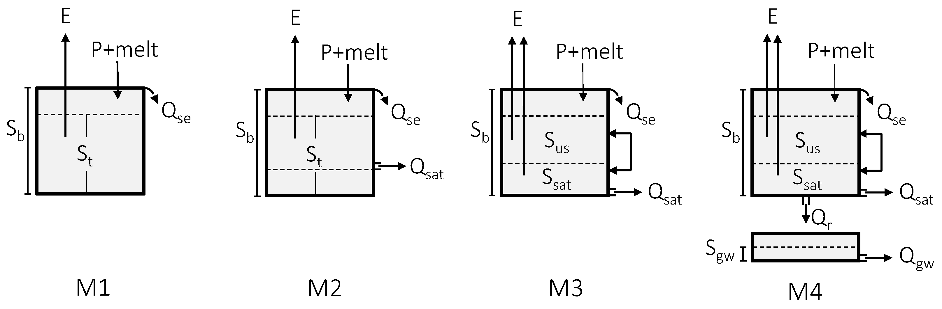
The hydrological models used in this study were developed by Atkinson et al. [53] and Farmer et al. [54] and later modified by Bai et al. [55] (Figure 3). The objective of using four hydrological models is to test if the main results and conclusions are sensitive to the hydrological model used. The results chapter focuses thus on the results of the most complex model (M4) and only considers the results obtained with the three simpler models in the final stage. Figure 3 shows a scheme of the models. Model M4 consists of a soil bucket which loses water through evapotranspiration (Esat and Eus), saturation excess flow (Qse), subsurface flow (Qsat) and percolation flow (Qr). The percolated water is captured by a groundwater reservoir and released as baseflow (Qgw). Evapotranspiration is modelled separately for the parts of the catchment covered by deep-rooted vegetation and the parts covered by bare soil and shallow roots. The soil bucket further distinguishes a saturated and an unsaturated zone, which interact differently with the potential evapotranspiration (PET) and therefore result in different actual evapotranspiration estimates. The PET was calculated in a previous study according to the Hargreaves and Samani [56] approach and used directly as input to the hydrological models. The PET does therefore not vary with the considered forcing. More information about models M1 to M3, which are basically simpler versions of this model, can be found in the studies referenced above.
3.4. Model Setup, Calibration and Evaluation
Model performance is analyzed in three stages, allowing a stepwise assessment of the changes in performance when moving from gauged to ungauged catchments. In the first step discharge data is used for calibrating all (snow and soil) parameters. The second step uses the soil parameters calibrated in the previous step but estimates the snow parameters without making use of the discharge data. In the final step, the discharge data is not used as all parameters are estimated based on other data sources. A sketch of the workflow is shown in Table 2 and a more detailed account of each step is presented below.
First step: Calibration of all parameters using discharge data (SCE parameters). For an initial assessment of model performance, the M4 hydrological model was calibrated with each combination of snowmelt model and forcing. The calibration was carried out with the SCE algorithm [57] using the mean absolute error (MAE) of the daily streamflow as objective function. The reason for choosing the MAE is that it gives the same weight to all observations, while an objective function squaring the error terms would have assigned a higher weight to the larger errors often observed at the hydrograph peaks. As in the current study many of these peaks will be caused by snowmelt, it was deemed a good idea to choose an objective function which does give such a large focus to the peaks (as it is the task of the snow models to correctly reproduce the snowmelt peaks). Instead, the calibration should focus on achieving a good performance during the periods less affected by snowmelt. These parameter values obtained by calibration to the discharge values will be identified as SCE parameters.
Second step: Estimation of the snow parameters without using discharge data. This stage informs about the model performance that can be achieved with the soil parameters calibrated in the previous step and with snow parameters estimated without using discharge data. The snow parameters were estimated with three approaches:
- An a priori estimate (Ap) based on literature data. A value of 1.7 °C was assigned to the snow/rain accumulation threshold () and the melt temperature () was set at 0 °C. Day-degree factors of 6 and 2 mm·°C−1·day−1 were used with the temperature-based and enhanced temperature-based approaches, respectively.
- An estimation of the snow parameters using the SNODAS data. Since this data is available for the whole US it represents a viable alternative for estimating the snow parameters in ungauged basins. For estimating the melt temperature, all days with snowmelt need to be identified. The minimum and maximum temperatures provided by each forcing (Livneh, MERRA-2) on these days are then retrieved. For ensuring that the identified temperatures are representative of the temperature at which snowmelt starts, only the temperature in the first day is considered when considered when melt takes place on consecutive days. The median temperature was assumed to be the melt temperature. A similar approach was used for the snow accumulation temperature, estimated as the median temperature for the days with a positive increase in the snow water equivalent. The day-degree factor was calibrated by fitting the snowmelt to the SNODAS melt. These parameters, obtained by calibrating the SNODAS data to the average daily temperatures, are identified as SD_av parameters.
- While snow parameters are usually estimated for the mean daily temperature, some studies suggest that the maximum temperature could be more appropriate [5,14]. Therefore, the snow parameters were additionally estimated using the same approach outlined above, but considering the maximum, instead of the mean daily temperatures. These parameters are abbreviated as SD_x parameters.
Third step: All parameters are estimated without using discharge data In the third step all parameters were estimated without relying on discharge data, which would be the situation encountered when modelling ungauged basins. As the snow parameters were already estimated in the previous step, it was only necessary to estimate the soil parameters. These were estimated a priori following the approaches described in Table 3.
Regarding the metrics for assessing model performance, the initial intention was to analyze the three components into which the Nash–Sutcliffe efficiency (NSE) can be decomposed [64]. These are the bias (simulated minus observed values), correlation, and standard deviation error. However, since the correlation between the bias and standard deviation (0.89) as well as the correlation between the NSE and the correlation (0.95) turned out to be high, only the results for the bias and correlation are presented here. A brief overview about the obtained NSE values is available in the Supplementary Materials.
4. Results
4.1. Performance of Snowmelt Models for Gauged Basins
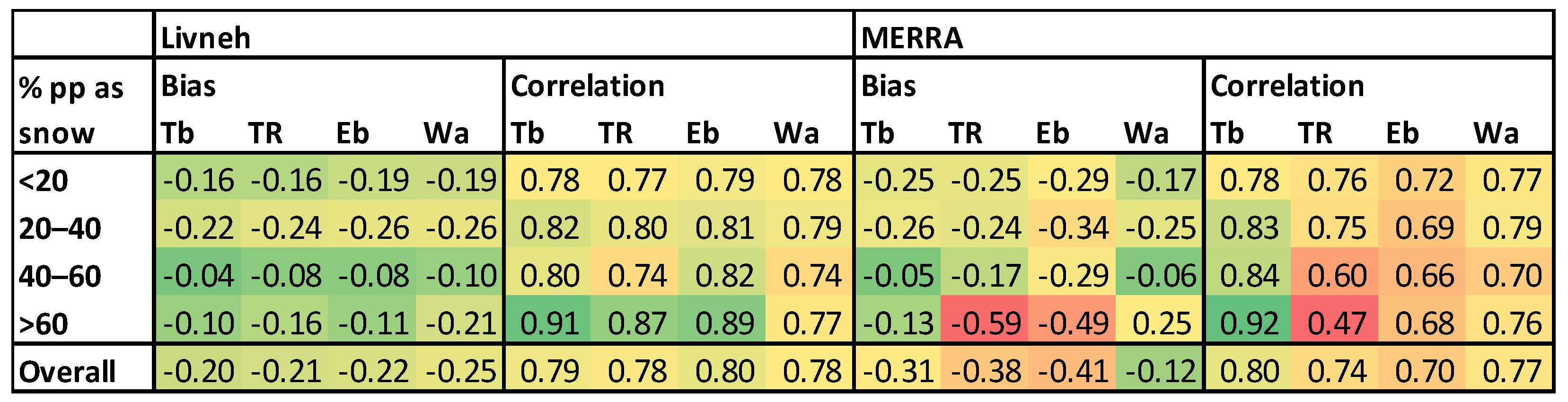
The performance (bias and correlation) achieved by the model M4 with the calibrated SCE parameters is presented in Figure 4. As expected, there are only small differences between models when the percentage of precipitation falling as snow is small, but the differences become more pronounced as the importance of snow increases.
The best results for the Livneh forcing are achieved with the temperature-based (Tb and TR) and the energy-balance (Eb) models, while the Walter (Wa) model has the worst performance, especially in catchments with much snow, reaching a median correlation of 0.77 and a mean annual bias of 77 mm (= 0.21 mm × 365 days) in catchments with over 60% of snow.
With the MERRA-2 forcing the Tb and Walter models reach a similar performance to the one obtained with the Livneh forcing. The TR and Eb models, on the other hand, show a marked decline in performance, especially in catchments with a high influence of snow. Since both models use radiation data, this suggests that there might be a problem with the radiation of the MERRA-2 forcing. While a detailed comparison of both forcings is beyond the scope of this study, it is helpful to have a detailed look at the net radiation, melt and modelled discharge in at least one catchment (Figure 5). Panel A shows that the net radiation estimated by the MERRA forcing starts to increase earlier after the winter and at a slower rate than the radiation from the Livneh forcing. This results in an earlier start of snow melt, smaller peaks (Panel B) and a hydrograph (red line) that does not match well the observed discharge (black line) (Panel C).
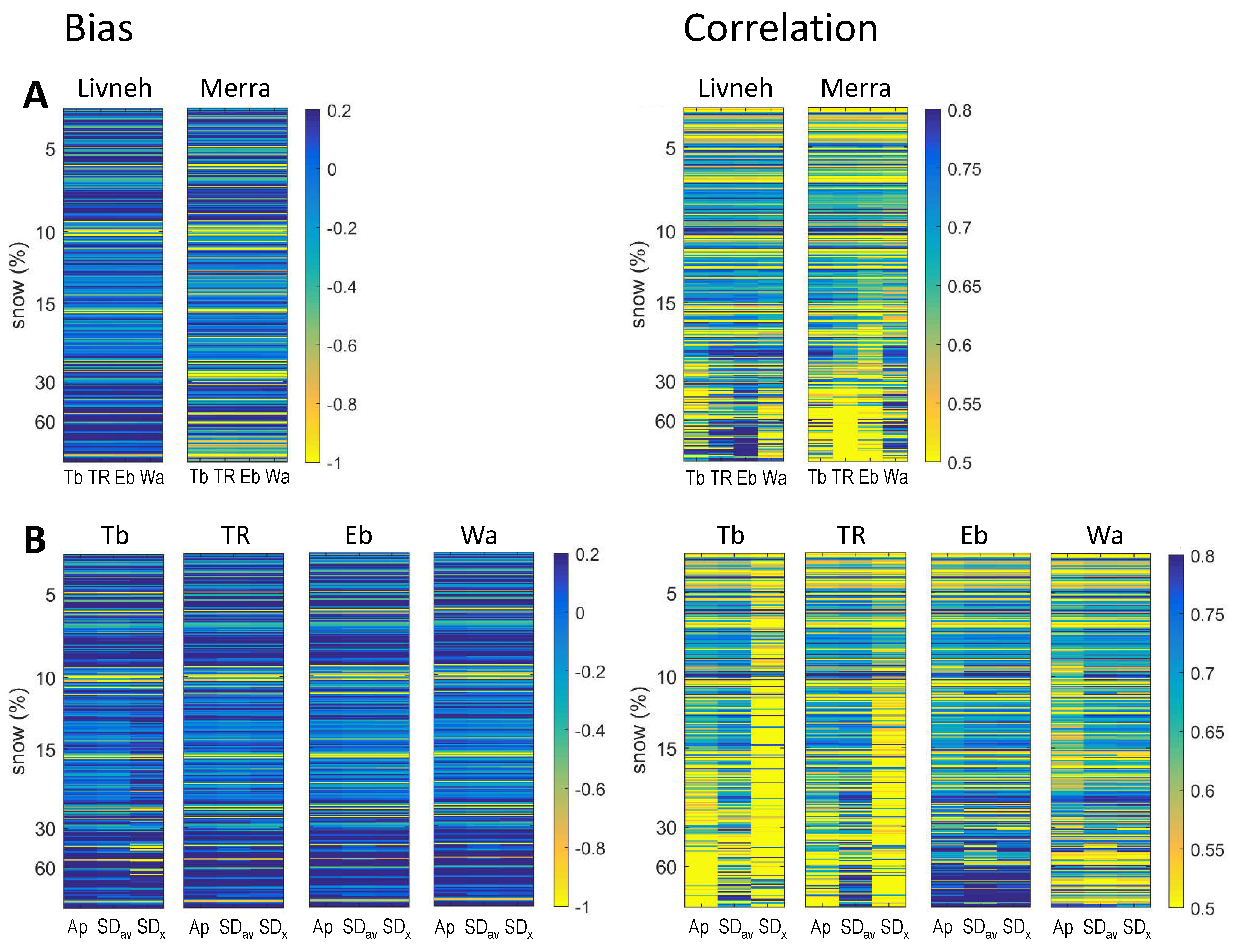
4.2. Performance of Snowmelt Models with Snow Parameters Estimated Without Using Discharge Data
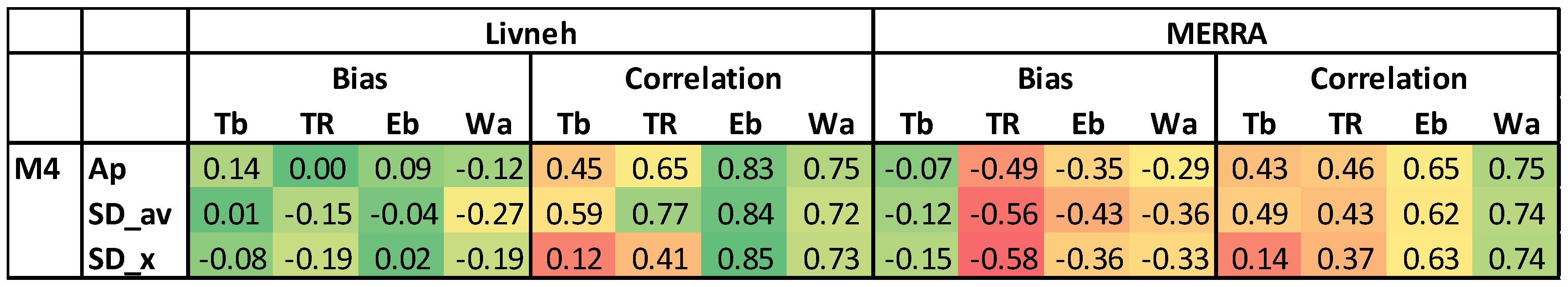
Figure 6 shows a summary of model performance when using the SCE calibrated soil parameters (from Section 4.1) and estimating the snow parameters in three different ways without using discharge data. The differences in bias and correlation between Figure 4 and the first row in Figure 6 show the decrease in performance observed when using a priori snowmelt parameters instead of calibrated parameters. It can be seen that the differences in bias are in most cases smaller than 0.2 mm. The decrease in correlation is small when considering energy-balance models, but temperature-based models, and here especially the traditional model (Tb), show large reductions in correlation.
The second row of Figure 6 allows assessing the impact of using the SNODAS data and the mean temperature (SD_av) for calibrating the snow parameters. In comparison with the a priori parameters there is in most cases an improvement in the correlation coefficient for the temperature snow models, while there is no positive effect on the correlation of the energy-balance models. For the bias, on the contrary, there is in most cases a decrease in performance.
Estimating the snow parameters using SNODAS and the maximum daily temperature (third row of Figure 6) does not result in any improvement, either in bias nor correlation, compared to the a priori estimated parameters.
Figure 7 shows the improvements in performance achieved when the snow parameters are estimated using the SNODAS dataset instead of using a priori estimates. It is seen that the a priori parameters result in large overestimations of the snowmelt peaks, especially for the temperature-based models. This can be successfully remedied using parameters estimated with the SNODAS data. The impact of using SNODAS calibrated parameters on the energy-balance models is much smaller. This can be explained by the number of calibrated parameters. While energy-balance models have only one snow parameter requiring calibration (accumulation temperature), temperature-based models have additionally the melt temperature and day-degree factor. This means that there is a larger potential for having a bad estimate if the a priori estimates are inadequate; on the other hand, there is also a larger potential for improvement.
4.3. Performance of Snowmelt Models for Ungauged Basins
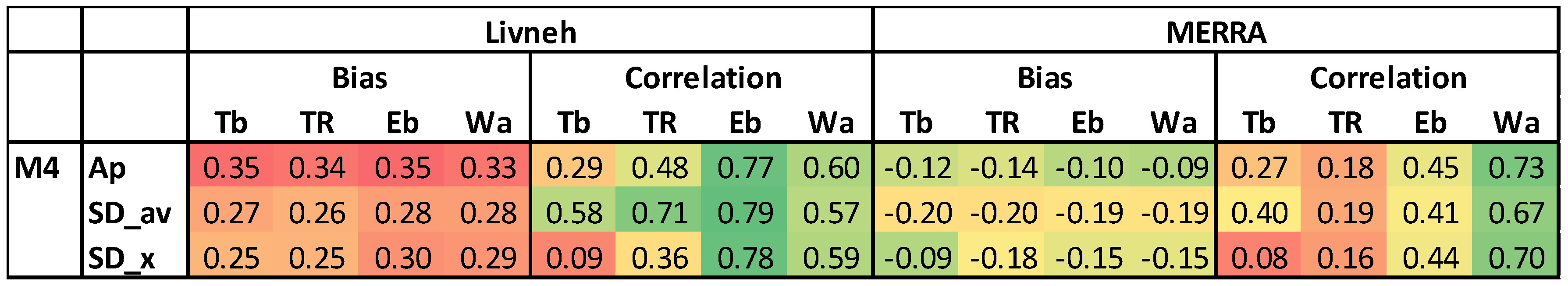
Figure 8 shows the results when modelling ungauged basins, i.e., when estimating snow and soil parameters without relying on discharge data. Bias has rather small differences between snow models and different approaches for estimating the snow parameters. There are, however, important differences between forcings, as the Livneh forcing results in positive biases, while the MERRA forcing gives negative ones.
When trying to rank the snow models with respect to correlation, it becomes clear that the adequacy of a given model will depend on (i) the quality of the input data (forcings) and (ii) the availability of additional data (SNODAS). The best correlation with the Livneh forcing is achieved with the energy-balance (Eb) model, which is the second-best model depends on the access to additional data. If the snow parameters can be calibrated using SNODAS data (SD_av), it is possible to achieve a good performance with the temperature-based models. In this case, the enhanced temperature model (TR) would be a better choice than the Walter model. If this were not the case, the Walter model would be preferred.
The situation is different when using the MERRA forcing. Because the radiation data seems to have some problems, neither the energy-balance (Eb) nor the enhanced temperature-based (TR) models can achieve high correlations. The best alternative then is to use the Walter model (Wa) which estimates the energy balance using only temperature data. Analogously to the results in Figure 6, the snow parameters estimated with the SNODAS data and the maximum daily temperatures (SD_x) do not improve model performance.
Figure 6 shows only the median performance for catchments with more than 40% of precipitation falling as snow. For analyzing the performance of all catchments and getting an idea about the variability in performance, the results of all catchments are shown in Figure 9. As already seen before, there are almost no differences in bias between the snow models and snow calibration approaches, but there are differences between the forcings, especially in catchments with a high influence of snow (Panel A). Correlation shows only a small variability between forcings and snow models when snow is not important (Panel A). For catchments with a high influence of snow, we see larger differences in the performance between forcings. Depending on how the snow parameters were estimated, there can be large differences in correlation even for catchments with a small impact of snow (Panel B). This is especially evident for the temperature-based models (Tb and TR).
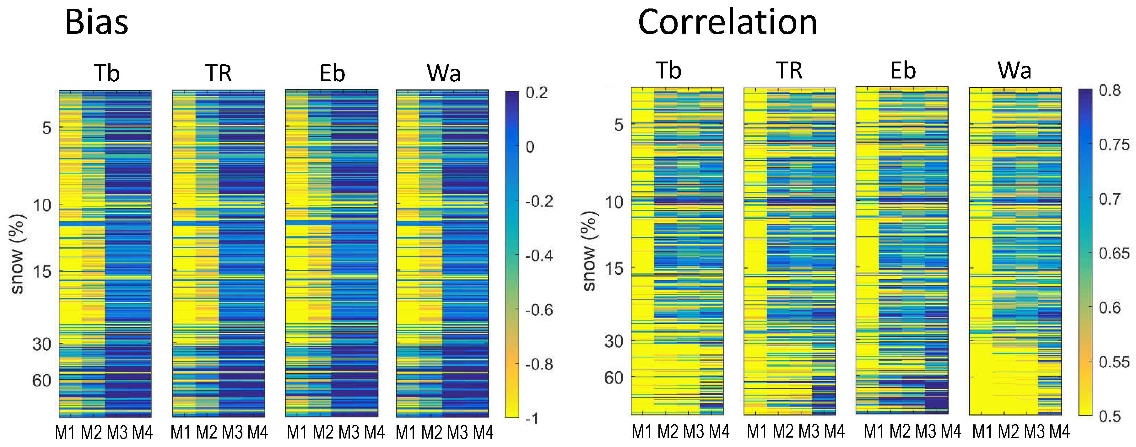
4.4. Consistency of Results for other Hydrological Models
This section looks at the impact of using other hydrological models. Figure 10 shows that bias is more affected by the choice of the hydrological model than by the choice of the snowmelt model. Specifically, it is seen that the biases in models M1 and M2 tend to be large in comparison to models M3 and M4. Also, for the correlation it is possible to see a clear impact of the hydrological model, as correlation is low for all catchments when using model M1. The remaining models do not exhibit large correlation differences between in catchments with little impact of snow. For the catchments with a higher proportion of snow there is a clear impact of the choice of the hydrological model on the achieved correlation.
5. Discussion
This study compared the performance of two temperature-index-based and two energy-balance models regarding their ability for reproducing the correlation and the bias between the observed and simulated discharge in 312 US catchments. The analysis considers the impact of using different forcings, approaches for calibrating the snow models and hydrologic models.
5.1. Performance with Respect to Correlation
An important result of this study is that the performance with respect to correlation depends on both: the snow and the hydrologic model. It can be seen that a hydrologic model that is too simple does not allow achieving a good correlation regardless of the considered snow model. The highest correlation was observed when using the most complex hydrologic model, stressing the need for using a model that has an adequate complexity.
The differences in correlation between the snow models are small when there is discharge data for calibrating the parameters and the input data is of good quality. This agrees with previous studies stating that the differences between temperature and energy-balance models are small when modelling gauged basins. As this study considered two forcings, one of which seems to have problems with the radiation data, it was possible to see the impact of having low quality data. The results clearly show that radiation data of low quality has a negative impact on performance in the models that use radiation data as input.
In ungauged catchments modelled with good quality climate data, the best correlation is achieved with energy-balance models. Classic temperature-based models (Tb), followed by the TR model, have the lowest correlations. The performance of the temperature-based models can be, however, considerably improved when SNODAS data is used for calibrating the snow parameters.
5.2. Performance with Respect to Bias
Bias is only marginally affected by the choice of the snowmelt model when modelling gauged basing with high quality forcing data. On the contrary, if radiation data is not of good quality, there can be large differences in bias between the snowmelt models, depending on their reliance on measured radiation data (Figure 4). While the impact of the snow parameters on bias is not large (compare Figure 4 and Figure 6), the soil parameters do have a large influence (compare Figure 6 and Figure 8). This is not surprising, as snowmelt models affect primarily the timing of snowmelt, and not the amount of melted water. The large impact of the structure (Figure 10) and parameterization (compare Figure 6 and Figure 8) of the hydrologic models can be explained by differences in the water balance caused by variations in the distribution and timing of flow. This results in specific soil moisture patterns interacting differently with the potential evapotranspiration which are finally reflected in unequal fractions of evapotranspiration and runoff.
Another factor affecting bias is the precipitation input. Figure 8 shows, for example, that the model driven by the Livneh and MERRRA-forcing data using a priori parameters have an average bias of about 0.35 and −0.11 mm·day−1, respectively. While bias is also affected by differences in temperature (as temperature influences the a priori snow parameters), it was previously shown that the impact of the snowmelt models was minor, so most of the differences in bias can be attributed to the precipitation input and differences in the evaporation. A comparison of the mean annual precipitation for the basins with more than 50% of solid precipitation between 1 October 2003 and 31 November 2011 showed that the mean annual precipitation of these basins reached 596 and 507 mm for the Livneh and MERRA-2 forcings, respectively. This is consistent with the sign of the bias as the Livneh forcing has a positive bias, indicating the simulated discharge is larger than the observed discharge. The MERRA-2 forcing, on the other hand, has a negative bias, meaning that the simulated discharge is smaller than the observed one.
An analysis of the precipitation input of the SNODAS product suggests, however, that both datasets (MERRA-2 and Livneh) might be underestimating precipitation. The sum of the rain- and snowfall of the hydrological models used as input for the SNODAS product, indicate that the average annual precipitation equals 491 mm. However, the sum of the inferred rainfall and melt—which is estimated using SWE values corrected by remote sensing data (among other data sources)—is 1040 mm. Since the Livneh forcing was obtained by interpolating measured observations from about 20,000 US climate stations with observation records larger than 20 years, its results will depend partly on the quality of the measured precipitation. Studies carried out in the US have found that gauges have an undercatch bias between 3% and 10% for rainfall and between 20% to 50% for snowfall [65,66]. Since snow undercatch tends to increase with increasing wind velocities, its impact increases at higher elevations and in mountainous areas. Snow undercatch in the stations used for deriving the Livneh forcing could be, therefore, responsible for the lower precipitation compared to the SNODAS product. The MERRA-2 dataset is the result of a reanalysis, i.e., it is the output of a climate model, which tend to have difficulties in getting good precipitation estimates. One reason for this is that precipitation estimates depend strongly on the model physics, known to have parameterization errors, and which can be very sensitive to small changes in the temperature and moisture fields [45]. Also the fact that precipitation is not a control variable in climate reanalyses, but a derived variable [44], explains the larger errors. The situation is different for the MERRA-2 dataset, as it delivers a bias corrected precipitation dataset besides the precipitation of the climate model output [67]. As this study uses the bias corrected precipitation, the precipitation amounts are similar to the precipitation of the Livneh dataset and it is expected that also the MERRA-2 precipitation might be affected by snow undercatch.
The large uncertainties in the precipitation estimates of the Livneh and MERRA-2 forcings due to snow undercatch and the important differences between the precipitation estimated by these datasets and the SNODAS estimates, stress that we are far from having certainty about the relative importance and magnitude of different components of the water balance [68]. A reduction in the bias of discharge estimates in ungauged basins can be therefore only expected once we have better estimates of these components.
5.3. MERRA-2 Radiation
Section 5.1 discussed model performance when considering different sources of radiation data. The MERRA-2 radiation data was regarded as being of lower quality than the Livneh data, since it resulted in a considerably lower performance with respect to correlation. An independent evaluation of the quality of the MERRA-2 radiation was carried out with the EBAF (Energy Balanced and Filled) datasets. This dataset is obtained by post-processing satellite measurements which aim at improving our understanding of the earth’s radiation budget. The results of the analysis are presented in the Supplementary Materials. They show that the MERRA-2 radiation agreed better with the EBAF radiation than with the Livneh radiation. As the EBAF and the MERRA-2 datasets have a much lower spatial resolution than the Livneh forcing, it is possible that the higher performance of the latter dataset can be explained by a better reproduction of the local radiation patterns. The performance differences might thus be the result of the different spatial resolutions more than due to deficiencies of the MERRA-2 dataset.
5.4. Limitations of the Study
This study implemented simple energy-balance models. It is possible that more sophisticated energy-balance models and approaches for estimating parameters in ungauged basins could have resulted in higher correlation values. Previous studies found, however, that such simple models might be adequate for estimating snowmelt, indicating that the improvement in performance might not be that significant [69].
In this study, the TR and Eb models used the radiation obtained from the Livneh and MERRA datasets as input, while the Wa model estimated the radiation terms based on temperature data. A more detailed comparison between these three snowmelt approaches should compare model performance of each model using the radiation from the forcing datasets and estimating the radiation input.
This study neglected snow losses due to sublimation and evaporation in all models for making results more comparable. As latent heat fluxes are explicitly calculated in energy-balance models, they are often included in these models, but not in day-degree snow models.
Supplementary Materials
The following are available at https://www.mdpi.com/2073-4441/11/2/301/s1.
Funding
This research was funded by the Austrian Science Fund (FWF): project J-3689-N29.
Acknowledgments
Ross Woods was available for discussions, provided comments on the manuscript and helped in the development of the procedures for estimating the a priori parameters.
Conflicts of Interest
The author declares no conflict of interest.
References
- Ferguson, R.I. Snowmelt runoff models. Prog. Phys. Geogr. 1999, 23, 205–227. [Google Scholar] [CrossRef]
- Barnett, T.P.; Adam, J.C.; Lettenmaier, D.P. Potential impacts of a warming climate on water availability in snow-dominated regions. Nature 2005, 438, 303–309. [Google Scholar] [CrossRef] [PubMed]
- Behnke, R.; Vavrus, S.; Allstadt, A.; Albright, T.; Thogmartin, W.E.; Radeloff, V.C. Evaluation of downscaled, gridded climate data for the conterminous United States. Ecol. Appl. 2016, 26, 1338–1351. [Google Scholar] [CrossRef] [PubMed]
- Hock, R. Temperature index melt modelling in mountain areas. J. Hydrol. 2003, 282, 104–115. [Google Scholar] [CrossRef]
- Corps of Engineers U.S. Army. Snow Hydrology. In Summary Report of the Snow Investigations; North Pacific Division: Portland, OR, USA, 1956. [Google Scholar]
- Martinec, J.; Rango, A. Parameter values for snowmelt runoff modelling. J. Hydrol. 1986, 84, 197–219. [Google Scholar] [CrossRef]
- Martinec, J.; de Quervain, M.R. The effect of snow displacement by avalanches on snow melt and runoff. IAHS-AISH 1975, 104, 364–377. [Google Scholar]
- Nolin, A.W. Recent advances in remote sensing of seasonal snow. J. Glaciol. 2010, 56, 1141–1150. [Google Scholar] [CrossRef]
- Dietz, A.J.; Kuenzer, C.; Gessner, U.; Dech, S. Remote sensing of snow—A review of available methods. Int. J. Remote Sens. 2012, 33, 4094–4134. [Google Scholar] [CrossRef]
- Walter, M.T.; Brooks, E.S.; McCool, D.K.; King, L.G.; Molnau, M.; Boll, J. Process-based snowmelt modeling: Does it require more input data than temperature-index modeling? J. Hydrol. 2005, 300, 65–75. [Google Scholar] [CrossRef]
- Franz, K.J.; Hogue, T.S.; Sorooshian, S. Operational snow modeling: Addressing the challenges of an energy balance model for National Weather Service forecasts. J. Hydrol. 2008, 360, 48–66. [Google Scholar] [CrossRef]
- Debele, B.; Srinivasan, R.; Gosain, A.K. Comparison of process-based and temperature-index snowmelt modeling in SWAT. Water Resour. Manag. 2010, 24, 1065–1088. [Google Scholar] [CrossRef]
- Dai, A. Temperature and pressure dependence of the rain-snow phase transition over land and ocean. Geophys. Res. Lett. 2008, 35, L12802. [Google Scholar] [CrossRef]
- Rajagopal, S.; Harpold, A.A. Testing and improving temperature thresholds for snow and rain prediction in the Western United States. J. Am. Water Resour. Assoc. 2016, 52, 1142–1154. [Google Scholar] [CrossRef]
- L’Hôte, Y.; Chevallier, P.; Coudrain, A.; Lejeune, Y.; Etchevers, P. Relationship between precipitation phase and air temperature: Comparison between the Bolivian Andes and the Swiss Alps. Hydrol. Sci. J. 2005, 50, 989–997. [Google Scholar] [CrossRef]
- Martinec, J. Snowmelt—Runoff model for stream flow forecasts. Hydrol. Res. 1975, 6, 145–154. [Google Scholar] [CrossRef]
- Ohmura, A. Physical Basis for the Temperature-Based Melt-Index Method. J. Appl. Meteorol. 2001, 40, 753–761. [Google Scholar] [CrossRef]
- Lang, H.; Braun, L. On the information content of air temperature in the context of snow melt estimation. IAHS 1990, 190, 347–354. [Google Scholar]
- Valéry, A.; Andréassian, V.; Perrin, C. ”As simple as possible but not simpler”: What is useful in a temperature-based snow-accounting routine? Part 2—Sensitivity analysis of the Cemaneige snow accounting routine on 380 catchments. J. Hydrol. 2014, 517, 1176–1187. [Google Scholar] [CrossRef]
- Valéry, A.; Andréassian, V.; Perrin, C. ”As simple as possible but not simpler”: What is useful in a temperature-based snow-accounting routine? Part 1—Comparison of six snow accounting routines on 380 catchments. J. Hydrol. 2014, 517, 1166–1175. [Google Scholar] [CrossRef]
- Kustas, W.P.; Rango, A.; Uijlenhoet, R. A simple energy budget algorithm for the snowmelt runoff model. Water Resour. Res. 1994, 30, 1515–1527. [Google Scholar] [CrossRef]
- Kane, D.L.; Giek, R.E.; Hinzman, L.D. Snowmelt modeling at small Alaskan arctic watershed. J. Hydrol. Eng. 1997, 2, 204–210. [Google Scholar] [CrossRef]
- Kollat, J.B.; Reed, P.M.; Wagener, T. When are multiobjective calibration trade-offs in hydrologic models meaningful? Water Resour. Res. 2012, 48, W03520. [Google Scholar] [CrossRef]
- U.S. Department of Agriculture (USDA). National Engineering Handbook. Part 630 Hydrology, Chapter 11 Snowmelt; 2004. Available online: http://www.wcc.nrcs.usda.gov/ftpref/wntsc/H&H/NEHhydrology/ch11.pdf (accessed on 1 February 2019).
- Brubaker, K.; Rango, A.; Kustas, W. Incorporating radiation inputs into the snowmelt runoff model. Hydrol. Process. 1996, 10, 1329–1343. [Google Scholar] [CrossRef]
- Martinec, J. Hour-to-hour snowmelt rates and lysimeter outflow during an entire ablation period. IAHS 1989, 183, 19–28. [Google Scholar]
- Carenzo, M.; Pellicciotti, F.; Rimkus, S.; Burlando, P. Assessing the transferability and robustness of an enhanced temperature-index glacier-melt model. J. Glaciol. 2009, 55, 258–274. [Google Scholar] [CrossRef]
- Pelliccotti, F.; Brock, B.; Strasser, U.; Burlando, P.; Funk, M.; Corripio, J. An enhanced temperature-index glacier melt model including the shortwave radiation balance: Development and testing for Haut Glacier d’Arolla, Switzerland. J. Glaciol. 2005, 51, 573–587. [Google Scholar] [CrossRef]
- Hock, R. A distributed temperature-index ice-and snowmelt model including potential direct solar radiation. J. Glaciol. 1999, 45, 101–111. [Google Scholar] [CrossRef]
- Cazorzi, F.; Dalla Fontana, G. Snowmelt modelling by combining air temperature and a distributed radiation index. J. Hydrol. 1996, 181, 169–187. [Google Scholar] [CrossRef]
- Kumar, L.; Skidmore, A.K.; Knowles, E. Modelling topographic variation in solar radiation in a GIS environment. Int. J. Geogr. Inf. Sci. 1997, 11, 475–497. [Google Scholar] [CrossRef]
- Bartelt, P.; Lehning, M. A physical SNOWPACK model for the Swiss avalanche warning. Part I: Numerical model. J. Cold Regions Sci. Technol. 2002, 35, 123–145. [Google Scholar] [CrossRef]
- Shuttleworth, W.J. Terrestrial Hydrometeorology; Wiley & Sons: New York, NY, USA, 2012; p. 448. [Google Scholar]
- Tarboton, D.G.; Chowdhury, T.G.; Jackson, T.H. A Spatially distributed energy balance snowmelt model. In Biogeochemistry of Seasonally Snow-Covered Catchments; Proceedings of a Boulder Symposium, Boulder CO, USA, 3–14 July 1995; Tonnessen, K.A., Ed.; IAHS Publishing: Oxford, UK, 1995; Volume 228, pp. 141–155. [Google Scholar]
- Huintjes, E.; Sauter, T.; Schröter, B.; Maussion, F.; Yang, W.; Kropáček, J.; Buchroithner, M.; Scherer, D.; Kang, S.; Schneider, C. Evaluation of a coupled snow and energy balance model for Zhadang glacier, Tibetan Plateau, using glaciological measurements and time-lapse photography. Arct. Antarct. Alpine Res. 2015, 47, 573–590. [Google Scholar] [CrossRef]
- Herrero, J.; Polov, M.J.; Moñinov, A.; Losadav, M.A. An energy balance snowmelt model in a Mediterranean site. J. Hydrol. 2009, 371, 98–107. [Google Scholar] [CrossRef]
- Magnussonv, J.; Wever, N.; Essery, R.; Helbig, N.; Winstral, A.; Jonas, T. Evaluating snow models with varying process representations for hydrological applications. Water Resour. Res. 2015, 51, 2707–2723. [Google Scholar] [CrossRef]
- Fuka, D.R.; Walter, M.T.; Archibald, J.A.; Steenhuis, T.S.; Easton, Z.M. EcoHydRology: A Community Modeling Foundation for Eco-Hydrology. R Package Version 0.4.12. Available online: http://CRAN.R-project.org/package=EcoHydRology (accessed on 1 February 2019).
- Bristow, K.L.; Campbell, G.S. On the relationship between incoming solar radiation and daily maximum and minimum temperature. Agric. For. Meteorol. 1984, 31, 150–166. [Google Scholar] [CrossRef]
- Rosenberg, N.J. Microclimate: The Biological Environment; Wiley: New York, NY, USA, 1974; p. 495. [Google Scholar]
- Wolock, D.M. Base-Flow Index Grid for the Conterminous United States. USGS Report 2003-263; 2003. Available online: http://pubs.er.usgs.gov/publication/ofr03263 (accessed on 1 February 2019).
- Livneh, B.; Rosenberg, E.A.; Lin, C.; Nijssen, B.; Mishra, V.; Andreadis, K.M.; Maurer, E.P.; Lettenmaier, D.P. A long-term hydrologically based dataset of land surface fluxes and states for the conterminous United States: Update and extensions. J. Clim. 2013, 26, 9384–9392. [Google Scholar] [CrossRef]
- Maurer, E.P.; Wood, A.W.; Adam, J.C.; Lettenmaier, D.P.; Nijssen, B. A long-term hydrologically based dataset of land surface fluxes and states for the conterminous United States. J. Clim. 2002, 15, 3237–3251. [Google Scholar] [CrossRef]
- Rienecker, M.M.; Suarez, M.J.; Gelaro, R.; Todling, R.; Bacmeister, J.; Liu, E.; Bosilovich, M.G.; Schubert, S.D.; Takacs, L.; Kim, G.-K.; et al. MERRA: NASA’s Modern-Era Retrospective Analysis for Research and Applications. J. Clim. 2011, 24, 3624–3648. [Google Scholar] [CrossRef]
- Gelaro, R.; McCarty, W.; Suárez, M.J.; Todling, R.; Molod, A.; Takacs, L.; Randles, C.A.; Darmenov, A.; Bosilovich, M.G.; Reichle, R.; et al. The Modern-Era Retrospective Analysis for Research and Applications, Version 2 (MERRA-2). J. Clim. 2017, 30, 5419–5454. [Google Scholar] [CrossRef]
- Wang, T.; Hamann, A.; Spittlehouse, D.; Carroll, C. Locally downscaled and spatially customizable climate data for historical and future periods for North America. PLoS ONE 2016, 11, e0156720. [Google Scholar] [CrossRef] [PubMed]
- Barret, A.P. National Operational Hydrologic Remote Sensing Center SNOwData Assimilation System (SNODAS) Products at NSIC; Special Report 11; National Snow and Ice Data Center: Boulder, CO, USA, 2003. [Google Scholar]
- National Operational Hydrologic Remote Sensing Center. Snow Data Assimilation System (SNODAS) Data Products at NSIDC; National Snow and Ice Data Center: Boulder, CO, USA, 2004. [Google Scholar]
- Clow, D.W.; Nanus, L.; Verdin, K.L.; Schmidt, J. Evaluation of SNODAS snow depth and snow water equivalent estimates for the Colorado Rocky Mountains, USA. Hydrol. Process. 2012, 26, 2583–2591. [Google Scholar] [CrossRef]
- Hedrick, A.; Marshall, H.-P.; Winstral, A.; Elderv, K.; Yueh, S.; Cline, D. Independent evaluation of the SNODAS snow depth product using regional-scale lidar-derived measurements. Cryosphere 2015, 9, 13–23. [Google Scholar] [CrossRef]
- Artan, G.A.; Verdin, J.P.; Lietzow, R. Large scale snow water equivalent status monitoring: Comparison of different snow water products in the upper Colorado Basin. Hydrol. Earth Syst. Sci. 2013, 17, 5127–5139. [Google Scholar] [CrossRef]
- Guan, B.; Molotch, N.P.; Waliser, D.E.; Jepsen, S.M.; Painter, T.H.; Dozier, J. Snow water equivalent in the Sierra Nevada: Blending snow sensor observations with snowmelt model simulations. Water Resour. Res. 2013, 49, 5029–5046. [Google Scholar] [CrossRef]
- Atkinson, S.E.; Woods, R.A.; Sivapalan, M. Climate and landscape controls on water balance model complexity over changing timescales. Water Resour. Res. 2002, 38, 1314. [Google Scholar] [CrossRef]
- Farmer, D.; Sivapalan, M.; Jothityangkoon, C. Climate, soil, and vegetation controls upon the variability of water balance in temperate and semiarid landscapes: Downward approach to water balance analysis. Water Resour. Res. 2003, 39, 1035. [Google Scholar] [CrossRef]
- Bai, Y.; Wagener, T.; Reed, P. A top-down framework for watershed model evaluation and selection under uncertainty. Environ. Model. Softw. 2009, 24, 901–916. [Google Scholar] [CrossRef]
- Hargreaves, G.H.; Samani, Z.A. Estimating potential evapotranspiration. J. Irrig. Drain. Div. 1982, 108, 225–230. [Google Scholar]
- Duan, Q.; Sorooshian, S.; Gupta, V. Effective and efficient global optimization for conceptual rainfall-runoff models. Water Resour. Res. 1992, 28, 1015–1031. [Google Scholar] [CrossRef]
- Homer, C.; Dewitz, J.; Fry, J.; Coan, M.; Hossain, N.; Larson, C.; Herold, N.; McKerrow, A.; VanDriel, J.N.; Wickham, J. Completion of the 2001 National Land Cover Database for the Conterminous United States. Photogramm. Eng. Remote Sens. 2007, 73, 337–341. [Google Scholar]
- Wang-Erlandsson, L.; van der Ent, R.J.; Gordon, L.J.; Savenije, H.H.G. Contrasting roles of interception and transpiration in the hydrological cycle—Part 1: Temporal characteristics over land. Earth Syst. Dynam. 2014, 5, 441–469. [Google Scholar] [CrossRef]
- Pelletier, J.D.; Broxton, P.D.; Hazenberg, P.; Zeng, X.; Troch, P.A.; Niu, G.; Williams, Z.C.; Brunke, M.A.; Gochis, D. Global 1-Km Gridded Thickness of Soil, Regolith, and Sedimentary Deposit Layers; ORNL DAAC: Oak Ridge, TN, USA, 2016. [Google Scholar]
- Chaney, N.W.; Wood, E.F.; McBratney, A.B.; Hempel, J.W.; Nauman, T.W.; Brungard, C.W.; Odgers, N.P. POLARIS: A 30-meter probabilistic soil series map of the contiguous United States. Geoderma 2016, 274, 54–67. [Google Scholar] [CrossRef]
- Merz, R.; Blöschl, G. Regionalization of catchment model parameters. J. Hydrol. 2004, 287, 95–123. [Google Scholar] [CrossRef]
- Parajka, J.; Viglione, A.; Rogger, M.; Salinas, J.L.; Sivapalan, M.; Blöschl, G. Comparative assessment of predictions in ungauged basins—Part 1: Runoff-hydrograph studies. Hydrol. Earth Syst. Sci. 2013, 17, 1783–1795. [Google Scholar] [CrossRef]
- Gupta, H.V.; Kling, H.; Yilmaz, K.K.; Martinez, G.F. Decomposition of the mean squared error and NSE performance criteria: Implications for improving hydrological modelling. J. Hydrol. 2009, 377, 80–91. [Google Scholar] [CrossRef]
- Groisman, P.; Legates, D. The Accuracy of United States Precipitation Data. Bull. Am. Meteorol. Soc. 1994, 75, 215–227. [Google Scholar] [CrossRef]
- Rasmussen, R.; Baker, B.; Kochendorfer, J.; Meyers, T.; Landolt, S.; Fischer, A.; Black, J.; Thériault, J.; Kucera, P.; Gochis, D.; et al. How well are we measuring snow: The NOAA/FAA/NCAR winter precipitation test bed. Bull. Am. Meteorol. Soc. 2012, 93, 811–829. [Google Scholar] [CrossRef]
- Reichle, R.H.; Liu, Q.; Koster, R.D.; Draper, C.S.; Mahanama, S.P.; Partyka, G.S. Land surface precipitation in MERRA-2. J. Clim. 2017, 30, 1643–1664. [Google Scholar] [CrossRef]
- Oliveira, P.T.S.; Nearing, M.A.; Moran, M.S.; Goodrich, D.C.; Wendland, E.; Gupta, H.V. Trends in water balance components across the Brazilian Cerrado. Water Resour. Res. 2014, 50, 7100–7114. [Google Scholar] [CrossRef]
- Koivusalo, H.; Heikinheimo, M.; Karvonen, T. Test of a simple two-layer parameterisation to simulate the energy balance and temperature of a snow pack. Theor. Appl. Climatol. 2001, 70, 65–79. [Google Scholar] [CrossRef]
Figure 1.
Location of the considered catchments and percentage of precipitation falling as snow.

Figure 2.
Sketch of the snow models specifying the time series used as input (T: temperature; P: precipitation, R: radiation; RH: relative humidity).
Figure 2.
Sketch of the snow models specifying the time series used as input (T: temperature; P: precipitation, R: radiation; RH: relative humidity).

Figure 3.
Sketch of the hydrological models.

Figure 4.
Performance of snowmelt models (median of catchments) disaggregated by percentage of precipitation falling as snow (%pp as snow). Validation data for SCE calibration of model M4. The cells were color-coded using a green (good performance)—yellow—red (bad performance) scale.
Figure 4.
Performance of snowmelt models (median of catchments) disaggregated by percentage of precipitation falling as snow (%pp as snow). Validation data for SCE calibration of model M4. The cells were color-coded using a green (good performance)—yellow—red (bad performance) scale.

Figure 5.
Daily net radiation for each forcing in catchment 06622700 (Panel A). Daily snow melt (mm) for the enhanced temperature-based model (TR) estimated with both forcings using the SCE calibrated parameters (Panel B). Observed and modelled discharge using SCE calibrated parameters for both forcings and the a priori (Ap) estimated parameters for the MERRA forcing (see Section 4.2) (Panel C).
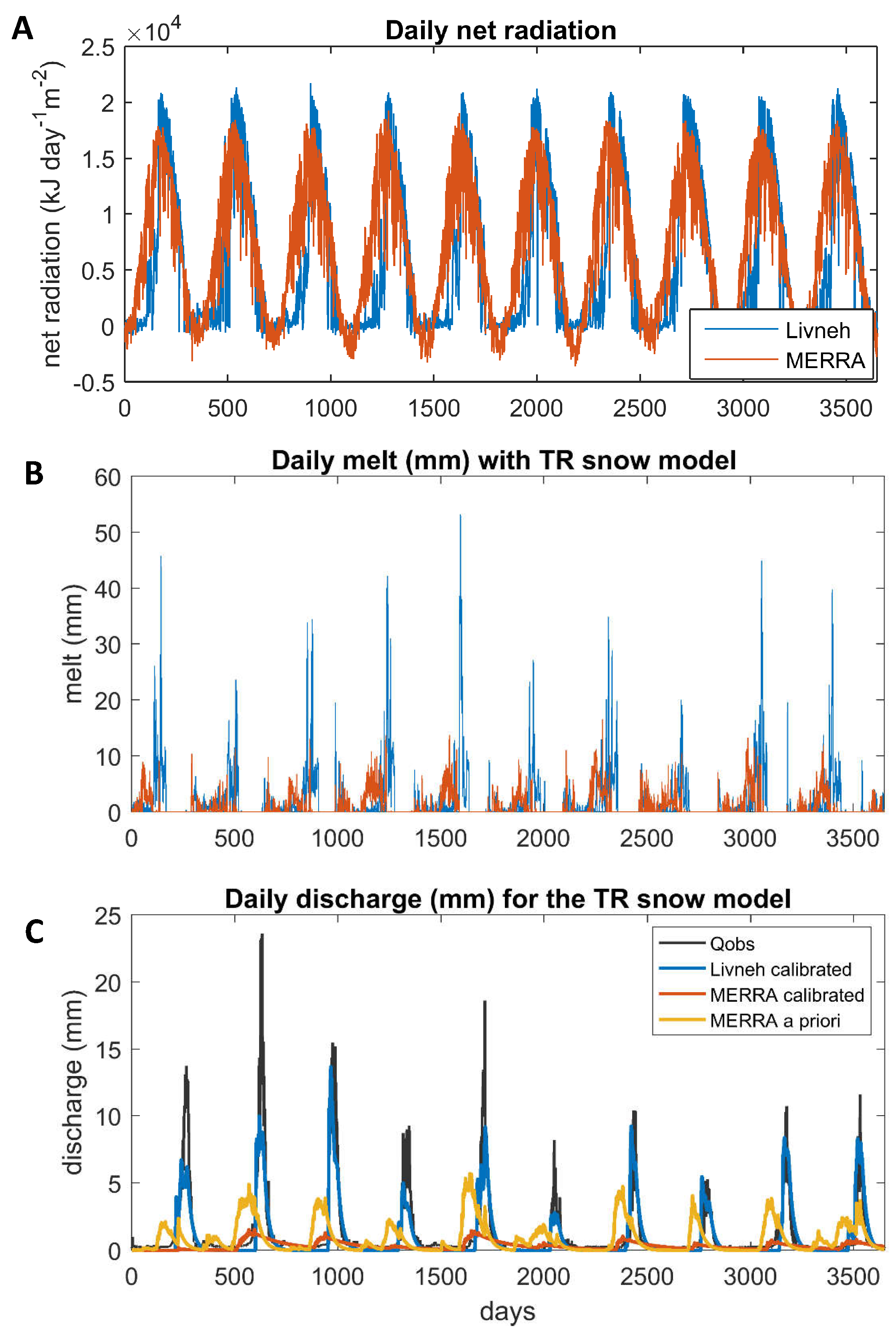
Figure 6.
Performance of snowmelt models (median of catchments) with the SCE calibrated soil parameters and with snow parameters estimated without using discharge data. Results for catchments with more than 40% of precipitation falling as snow. The cells were color-coded using a green (good performance)—yellow—red (bad performance) scale. The rows show the results using three approaches for estimating the snow parameters Ap (a priori); SD_av (using SNODAS data and the daily average temperature); SD_x (using SNODAS data and the daily maximum temperature).

Figure 7.
Hydrographs for all snow models with SCE calibrated soil parameters for catchment 12488500 which has 62% of precipitation falling as snow. The plots on the left use a priori estimated snow parameters; on the right, the snow models use the parameters estimated with SNODAS using the average daily temperature (SD_av).
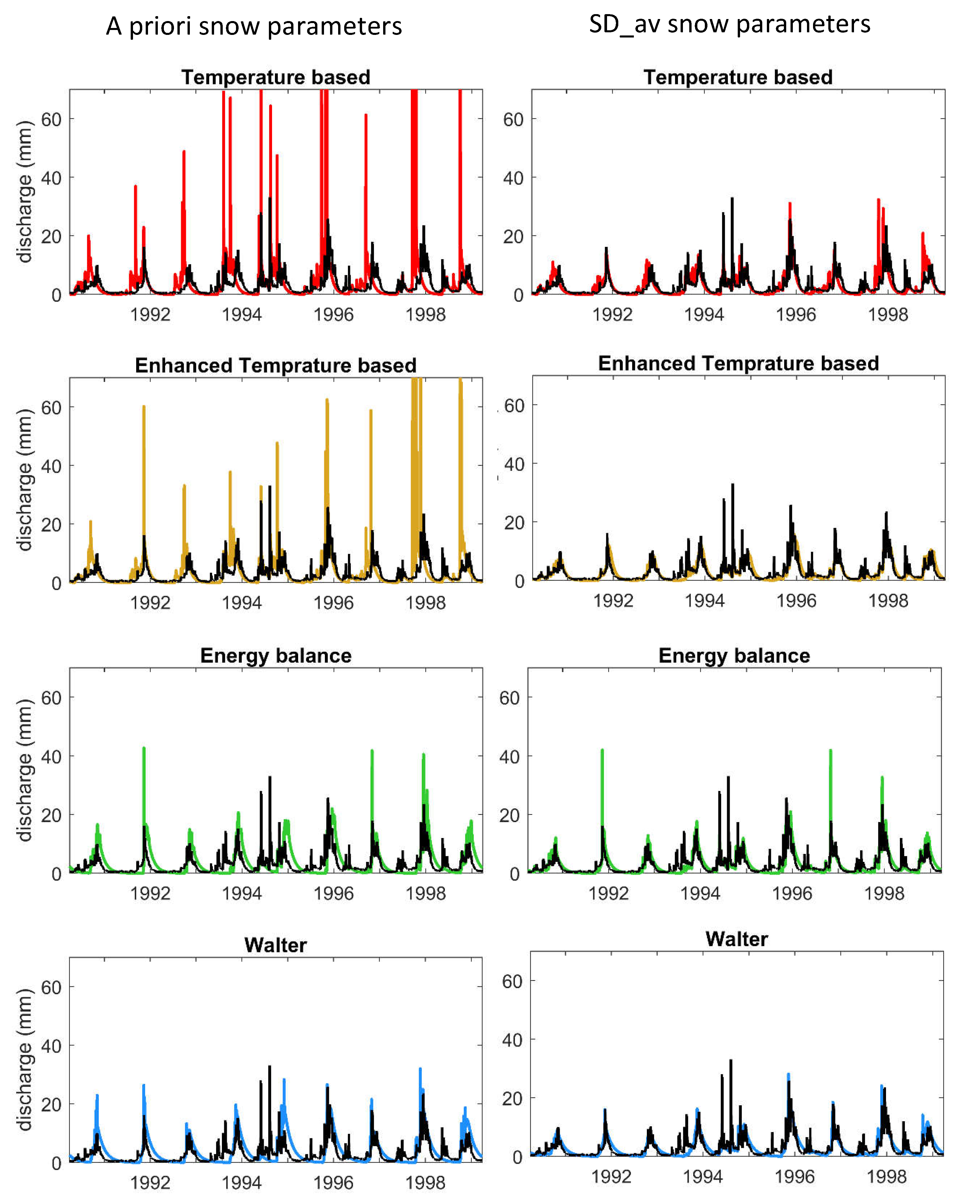
Figure 8.
Performance of snowmelt models (median of catchments) with soil and snow parameters estimated without using discharge data. Results for catchments with more than 40% of precipitation falling as snow. The cells were color-coded using a green (good performance)—yellow—red (bad performance) scale. The rows show the results using three approaches for estimating the snow parameters Ap (a priori); SD_av (using SNODAS data and the daily average temperature); SD_x (using SNODAS data and the daily maximum temperature).

Figure 9.
Bias and correlation for all catchments. Panel A: For both forcings and all snow models with the SD_av snow parameters. Panel B: For all snow models and all approaches for estimating the snow parameters. Unless otherwise stated, the M4 hydrological model driven by the Livneh forcing with a priori soil parameters was used.

Figure 10.
Bias and correlation for the snow models with the SD_av snow parameters and a priori soil parameters. All hydrological models are driven by the Livneh forcing.
Figure 10.
Bias and correlation for the snow models with the SD_av snow parameters and a priori soil parameters. All hydrological models are driven by the Livneh forcing.


Table 1.
Characterization of the considered catchments.
| Property | Unit | Min | Max | Median |
|---|---|---|---|---|
| snow | % | 3 | 87 | 15 |
| precipitation 1 | mm | 401 | 3314 | 1137 |
| temperature 1 | °C | −1.5 | 13.7 | 7.3 |
| PET 2 | mm | 615 | 1277 | 927 |
| area | km2 | 4 | 14,269 | 304 |
| elevation | m.a.s.l. | 14 | 3644 | 610 |
| forest | % | 0 | 99 | 69 |
| barren land | % | 0 | 40 | 0 |
| glacier | % | 0 | 52 | 0 |
| BFI 3 | - | 0.1 | 0.85 | 0.5 |
| discharge | mm | 14 | 3514 | 479 |
1 Estimated with Daymet 3 data; 2 Potential evaporation estimated using the Hargreaves and Samani formula; 3 Baseflow index provided by the USGS [41].
Table 2.
Summary of the options considered in the workflow.
| Analysis | Forcing | Snow Model | Soil Parameters | Snow Parameters |
|---|---|---|---|---|
| step 1 | Livneh MERRA | Tb TR Eb Wa | SCE calibration to discharge | SCE calibration to discharge |
| step 2 | Livneh MERRA | Tb TR Eb Wa | SCE calibration to discharge | 3 estimation approaches: a priori (Ap) and using SNODAS data (SD_av, SD_x) |
| step 3 | Livneh MERRA | Tb TR Eb Wa | A priori | 3 estimation approaches: a priori (Ap) and using SNODAS data (SD_av, SD_x) |
Table 3.
Description of the procedure estimating the soil parameters a priori.
| Parameter | Description of the a Priori Estimation Approach |
|---|---|
| M | Percentage of deep-rooted vegetation in the catchment Estimated as the percentage of the catchment covered by forests (evergreen, mixed and deciduous) according to the NLCD (National Land Cover Database) 2001 landcover [58]. |
| Interception coefficient Estimated as a function of the percentage of the catchment covered by different land use classes and the interception factors for each land use class provided by Wang-Erlandsson [59]. | |
| Size of soil storage The average thickness of the permeable rocks above bedrock was estimated using the Pelletier et al. [60] datasets. This was multiplied by the fraction of soil water between saturation and the permanent wilting point estimated with the POLARIS dataset [61]. | |
| Field capacity Estimated as a function of the soil properties obtained from the POLARIS datasets following the approach of [55]. | |
| Surface recession , recharge coefficient and baseflow recession Since there is no straightforward way of estimating these variables from the catchment properties we used the values from the nearest catchment (centroid) for which we had information. This is justified by previous studies indicating that geographical proximity provides good results when estimating parameters for ungauged basins [62,63]. |
© 2019 by the author. Licensee MDPI, Basel, Switzerland. This article is an open access article distributed under the terms and conditions of the Creative Commons Attribution (CC BY) license (http://creativecommons.org/licenses/by/4.0/).
Share and Cite
MDPI and ACS Style
Massmann, C. Modelling Snowmelt in Ungauged Catchments. Water 2019, 11, 301. https://doi.org/10.3390/w11020301
AMA Style
Massmann C. Modelling Snowmelt in Ungauged Catchments. Water. 2019; 11(2):301. https://doi.org/10.3390/w11020301
Chicago/Turabian StyleMassmann, Carolina. 2019. "Modelling Snowmelt in Ungauged Catchments" Water 11, no. 2: 301. https://doi.org/10.3390/w11020301
APA StyleMassmann, C. (2019). Modelling Snowmelt in Ungauged Catchments. Water, 11(2), 301. https://doi.org/10.3390/w11020301
Note that from the first issue of 2016, this journal uses article numbers instead of page numbers. See further details here.