Transmissibility Upscaling on Unstructured Grids for Highly Heterogeneous Reservoirs

Abstract

One critical point of modeling of flow in porous media is the capacity to consider parameters that are highly variable in space. It is then very challenging to simulate numerically fluid flow on such heterogeneous porous media. The continuous increase in computing power makes it possible to integrate smaller and smaller heterogeneities into geological models of up to tens of millions of cells. On such meshes, despite computer performance, multi-phase flow equations cannot be solved in an acceptable time for hydrogeologists and reservoir engineers, especially when the modeling considers several components in each fluid and when taking into account rock-fluid interactions. Taking average reservoir properties is a common approach to reducing mesh size. During the last decades, many authors studied the upscaling topic. Two different ways have been investigated to upscale the absolute permeability: (1) an average of the permeability for each cell, which is then used for standard transmissibility calculation, or (2) computing directly the upscaled transmissibility values using the high-resolution permeability values. This paper is related to the second approach. The proposed method uses the half-block approach and combines the finite volume principles with algebraic methods to provide an upper and a lower bound of the upscaled transmissibility values. An application on an extracted map of the SPE10 model shows that this approach is more accurate and faster than the classical transmissibility upscaling method based on flow simulation. This approach keeps the contrast of transmissibility values observed at the high-resolution geological scale and improves the accuracy of field-scale flow simulation for highly heterogeneous reservoirs. Moreover, the upper and lower bounds delivered by the algebraic method allow checking the quality of the upscaling and the gridding.

1. Introduction

One of the essential points for the hydrogeologists and the reservoir engineers is the transition from the geological mesh to the reservoir mesh. The properties of the reservoir mesh, being composed of cells supposed to represent an average of the properties of the geological model, affect the results of the simulations essential to solving different problems such as history matching, the optimization of the production, the production forecasting and their associated uncertainties [1]. This upscaling step is even more critical for geological reservoirs with high-heterogeneous properties, particularly for the management of aquifers (e.g., seawater intrusion in coastal aquifer [2]), the management of hydrocarbon reservoirs [3], or the geological sequestration of CO₂ [4,5].

Usually, geostatistical approaches are used to model the geological model and stochastically generate the distribution of the reservoir heterogeneity on meshes of tens of millions of cells. However, the numerical fluid flow simulations with commercial reservoir simulators are not conceivable with such mesh size. Despite the increase in computational speed, an averaging step of the heterogeneous properties is mandatory to reduce the mesh size and make it possible to perform multi-phase flow reservoir simulations.

Many authors have investigated several averaging methods of reservoir properties in the last decades [6,7,8,9]. Regarding the averaging of absolute permeability, these methods can be split into two categories:

(1)

Approach #1: first, the absolute permeability is averaged for each reservoir cell, and then the discretization of the flow equations lead computing the transmissibility values [10,11,12,13,14];

(2)

Approach #2: the average transmissibility values are calculated directly from the high-resolution scale permeability distributions [15,16,17,18,19,20].

Regardless of the approach chosen, the upscaling step leads to a loss of information. Different criteria have been proposed to quantify the error introduced by the upscaling step [21,22,23,24,25].

Generally, when the main flow direction is not parallel to the main axes of the grid, the average permeability should be represented by a full tensor for adequately taking into account the characteristics of the flow. But, the permeability obtained cannot be used directly in the discretized equation. A harmonic average between the permeability of two neighboring cells is then usually used to obtain the transmissibility values. Samier [15] proposes a finite element volume technique with schemes varying from 9 to 27 points, applied on non-uniform grid spacing. The framework developed by Ding and Urgelli [16] and Urgelli [17], deliver a technic to calculate the large-scale reservoir transmissibility values on a shifted block approach with a finite volume discretization of flow equation for Cartesian grids and corner point geometry (CPG) grids. In addition to the numerical scheme, the choice of the boundary condition differs according to the methods. The shifted block that has been proved in one dimension in space (1D) by Urgelli [17] to be more accurate than the use of full blocks (Approach #1).

Panfili et al. [19] have used upscaled transmissibility to a huge carbonate reservoir, the Kashagan field, located below the North Caspian Sea, and they have found this approach more accurate by numerical comparisons with simulations on high-resolution geological cells.

This paper follows the second approach. The half-cell volumes on both sides of the boundaries are taken into account to preserve the contrast of the heterogeneity better. Compared to previous works, the shifted block technique is considered, and the finite volume principles are combined with algebraic approaches to provide the two bounds (upper and lower) of the upscaled transmissibility values. The presented method uses a combined approach, including the advantages of algebraic methods and the flow-based method, i.e., the speed and accuracy. Moreover, the two bounds of the upscaled transmissibility values allow controlling the quality of upscaling and the gridding.

In the next section, the proposed approach is detailed, and the implementation steps are given. Then, to show the benefits of this method, a comparison of transmissibility estimation that we propose is done with the results obtains with the “classical” approach (Approach #1), on an extracted map of the SPE10 model.

2. Local Transmissibility Upscaling Method

The proposed transmissibility upscaling approach extends the algebraic upscaling method initially introduced by Guérillot et al. [11], called Cardwell and Parsons. We suggest a transmissibility upscaling version of this approach. This methodology, primarily based on the permeability upscaling techniques, enables the spatial distribution of local transmissibility values to be taken into account. The precision of the estimation is improved by considering the neighboring volumes on each side of the edge of the cells in a way leading to better preserves the transmissibility contrast introduced by the high-resolution geological cell-scale heterogeneities.

One of the benefits of the algebraic approach is that the upper and lower bounds are given: $T_{+}$ and $T_{-}$. The accuracy of the upscaling and the quality of the gridding process can be controlled using these boundaries. In addition, if $T_{+}$/$T_{-}$, the ratio of $T_{+}$ versus $T_{-}$ is lower than a specified given threshold, then the averaged transmissibility values proposed by Guérillot et al. [11] would be the geometric mean of these two bounds. This geometric mean degenerates well in the case where the arithmetic average or the harmonic average is the correct solution. A ratio of the bounds above this given threshold indicates that the griding must be redesigned.

Combining the half-block approach and the finite volume principles with algebraic methods, the introduced “local” method consists of:

(1)

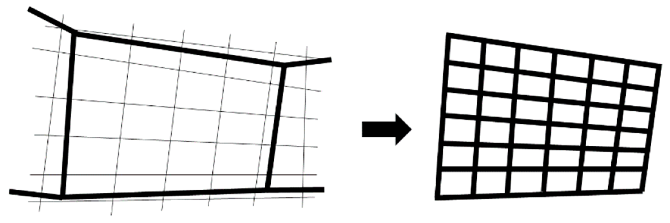
Remeshing each reservoir cell with a high-resolution geological mesh finer than the geological mesh;

(2)

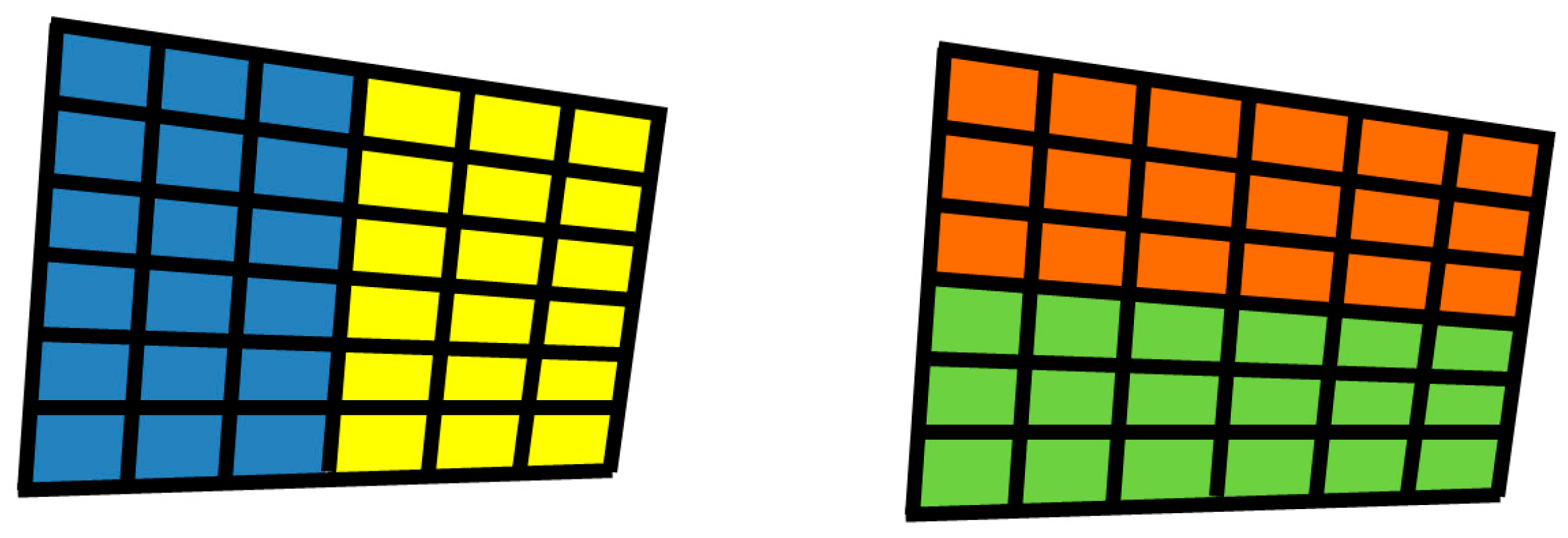
Decomposing each reservoir cell in local sub-domain containing geological cells;

(3)

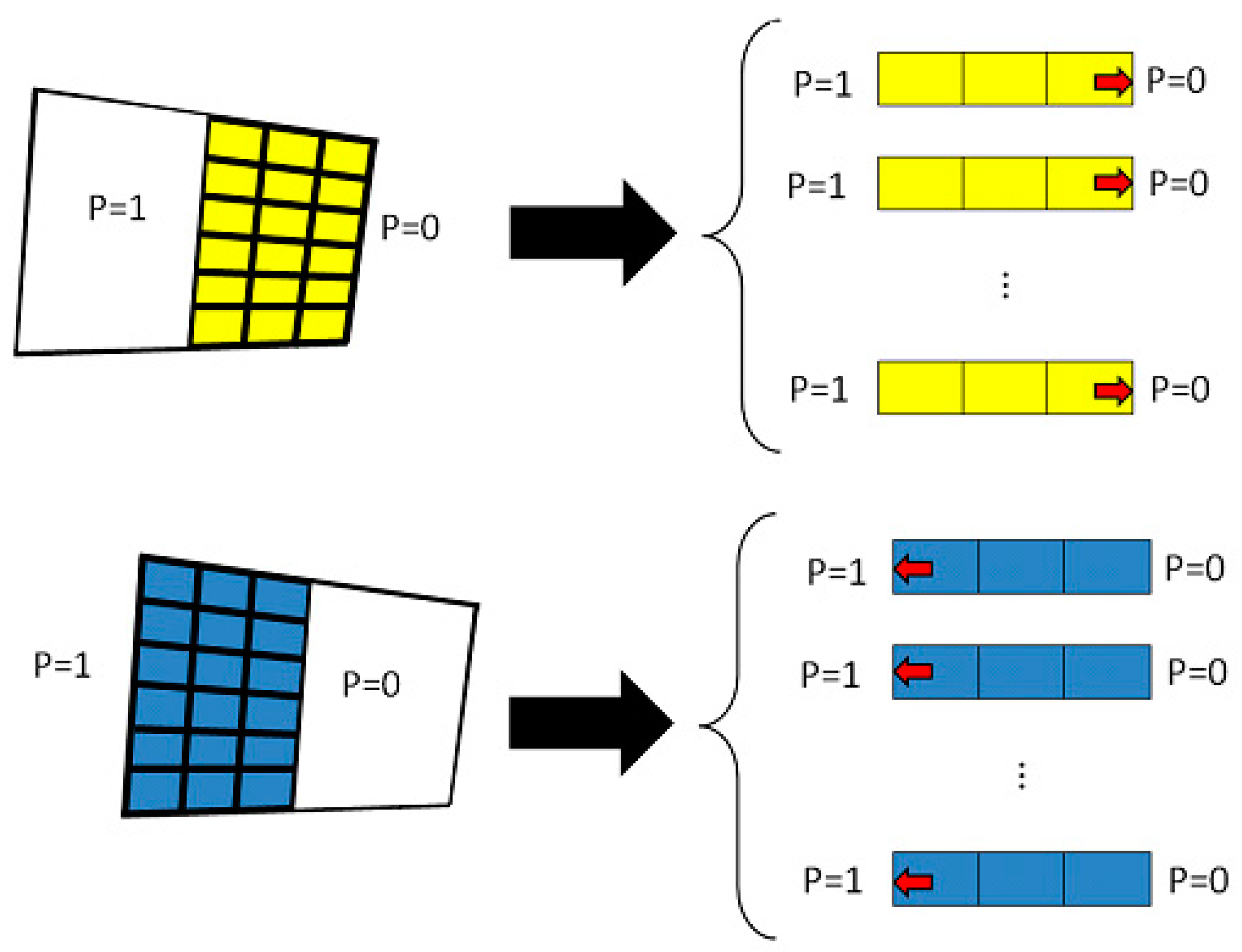
Calculate an upper and lower admissible half-transmissibility values on each sub-domain of each reservoir cell, by defining for each shifted block, 1D local problems with linear pressure boundary conditions [11] and apply a finite-volume numerical scheme to discretize these local problems;

(4)

Calculate upscaled transmissibility values between each reservoir cells using half-transmissibility values of corresponding cells weighted by the surface exchange between these cells.

Let us assume that the geological mesh refers to the ensemble of three-dimensions in space (3D) cells with their associated porosities and permeability tensor used to represent the geological model, that the simulator mesh can be built independently of the geological mesh, without constraint between both, and that the geological and reservoir mesh could be both built using cells represented by eight points in space without restrictions on their alignments. Throughout this paper, the lowercase refers to variables associated with the geological mesh and the capital letters to the reservoir mesh.

2.1. Remeshing

Each target cell (large reservoir cell), is refined with more cells than the source cells (high-resolution geological cells). The refining in I, J and K direction is done with an even cell number (cf. Figure 1).

For each source cells (high-resolution geological cells), sampling new high-resolution geological cells (large reservoir cell refined) is whose centers are contained in the source cell.

2.2. Sub-Domains Decomposition

The half parts of the blocks on each side of the boundaries of the two grid blocks are extracted to compute the upscaled transmissibility values. Six spatial domains are defined for each cell. Right and Left domains allow computing the I-Transmissibility values. North and South allow computing the J-Transmissibility values. Top and bottom domains allow computing the K-Transmissibility values. Figure 2 presents a 2D illustration of the domains. Then following a spatial clustering of permeability, a one-dimensional local flow-based transmissibility calculation is done to define the lower and upper bound transmissibility values. Below, details are given to explain how these bounds are obtained, and a final estimator for the transmissibility values associated with reservoir mesh is proposed.

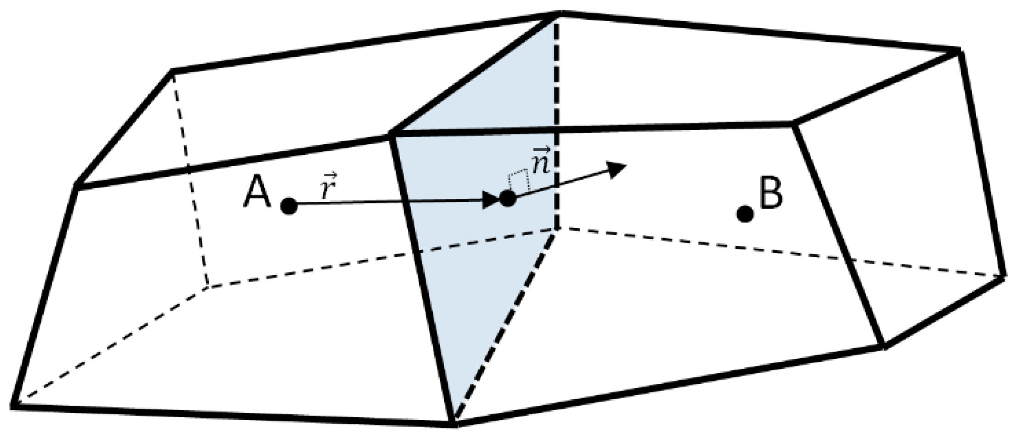
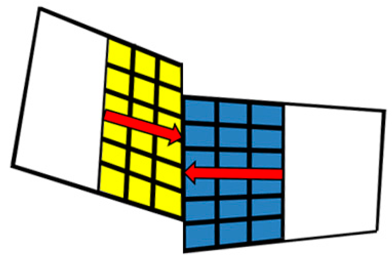
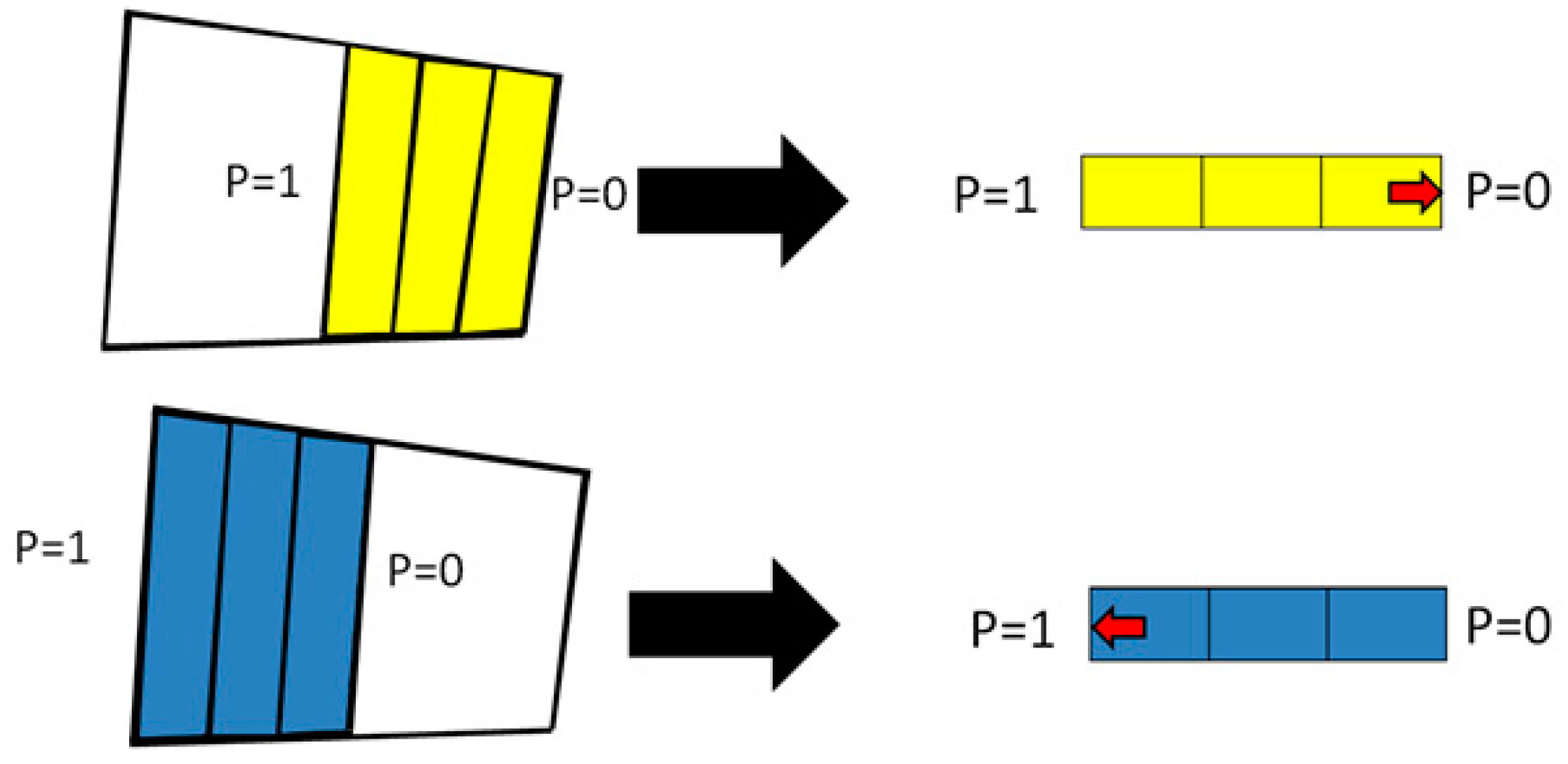
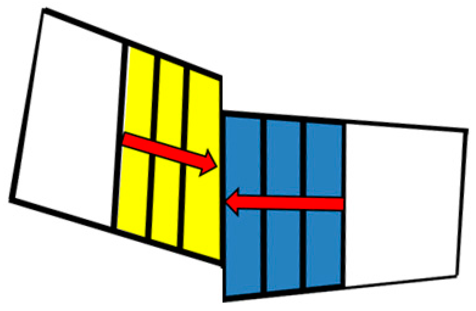
2.3. Lower and Upper Bounds Transmissibility

The transmissibility between two cells is given as follows:

$$t_{i,n\left(i\right)}={\left(\frac{1}{{\tau }_i}+\frac{1}{{\tau }_{n\left(i\right)}}\right)}^{-1},$$

(1)

where $\tau$ is the half-transmissibility for the neighboring cells $i$ and $n\left(i\right)$, defined as follows:

$${\tau }_{\alpha }=k_{\alpha }\frac{n_{\alpha }{s}_{AB}{r}_{\alpha }}{{\left|r_{\alpha }\right|}^2},\alpha =i,n\left(i\right),$$

(2)

where $k_{\alpha }$ is the permeability of the cell in the direction $\alpha$, $n_{\alpha }$ a normal vector to the interface, $s_{AB}$ the surface between the cells A and B, $r_{\alpha }$ the vector between the two centers: the cell center and the interface center (cf. Figure 3).

2.3.1. Implementation of the Lower Bound Transmissibility

For each local domain, with n high-resolution geological cells at the cell edge, the computation of the lower estimated bound value for the transmissibility is done considering n 1D steady-state incompressible flow.

The finite volume discretization of Darcy’s law for these one-dimensional systems can be written as follows:

$$t_{i-1,i} \left(p_{i-1} -p_i\right)+ t_{i,i+1} \left(p_{i+1} - p_i\right)=0 .$$

(3)

Dirichlet boundary conditions are defined to solve this system with a pressure equal to unity on one side and zero on the other side. After discretization in space, the following matrix system needs to be solved. It is particularly easy as it is a tri-diagonal symmetric matrix:

$$Au=b,$$

(4)

where $A$ is the matrix inclosing the transmissibility terms, $u$ the unknowns represented by a vector, and $b$ includes the boundary conditions. The dimension of the matrix $A$ is $\left(n_{ct}+2\right)\times \left(n_{ct}+2\right)$, $n_{ct}$ is the number of cells in each 1D system (cf. Figure 4).

The Darcy’s flux at the interface between the two cells gives:

$$q_{i,i+1}={\left(\tau \right)}_{i,i+1} \left(p_i-p_{i+1}\right) .$$

(5)

The half-transmissibility can be written as follows:

$$T_{\frac{1}{2}\left(\beta ,d\right)}^{-}={\displaystyle \sum }_n q_n ,$$

(6)

where $\beta$ is the index of a reservoir large cell, $d$ is the domain: right, left, north, south, top or bottom, $n$ is the number of high-resolution geological cells at the interface between the two large reservoir cells, and $q_n$ is the high-resolution scale flux.

The lower estimated bound value for the transmissibility between two given large reservoir cells A and B (cf. Figure 5) is defined as follows:

$$T_{-}={\left(\frac{1}{\frac{S_{AB}}{S_{A_d}}{T}_{\frac{1}{2}\left(A,d\right)}^{-}}+\frac{1}{\frac{S_{AB}}{S_{B_{\overline{d}}}}{T}_{\frac{1}{2}\left(B,\overline{d}\right)}^{-}}\right)}^{-1},$$

(7)

where $s_{AB}$ is the cell interface area between the cells A and B, $s_{A_d}$ is the total surface area between the cells A and the connected cells on the $d$ domain, $\overline{d}$ is the opposite domain of the domain $d$.

2.3.2. Implementation of the Upper Bound Transmissibility

To compute the upper bound transmissibility value, the cells are clustered to generate slices perpendicular to the considered direction for each local domain (cf. Figure 6).

The computation of the half-transmissibility value (Equation (2)) between two slices is done as follow:

• $k_{\alpha }$ is the arithmetic mean of the permeability for each slice perpendicular to the considered direction. The upper bound of the admissible permeability value and the exact value for a stratified medium considering a parallel flow is given by arithmetic mean of the permeability values;
• $n_{\alpha }$ is a normalized vector through each cell;
• $s$ is the sum of the areas of the interfaces of the high-resolution geological cells;
• $r_{\alpha }$ is the arithmetic mean of the vector connecting the centers of each high-resolution geological cell with the center of the interface.

Equation (1) allows calculating the transmissibility value across each slice. Then, the same strategy as the lower bound is applied, i.e., the computation of the upper estimated bound value for the transmissibility is done considering one steady-state incompressible 1D single-phase flow model without gravity. The pressure equation is solved considering Dirichlet boundary conditions with a pressure equal to unity on one side and zero on the other side.

The Darcy’s flux at the interface between the two cells can be written as follows:

$$q_{i,i+1}={\left(\tau \right)}_{i,i+1} \left(p_i-p_{i+1}\right) .$$

(8)

The half-transmissibility can be written as follows:

$$T_{\frac{1}{2}\left(\beta ,d\right)}^{+}=q ,$$

(9)

where $\beta$ is the index of the large reservoir cell, $d$ is the domain: right, left, north, south, top or bottom, and $q$ is the flux at the interface.

The upper estimated bound value for the transmissibility between two given large reservoir cells A and B (cf. Figure 7) can be defined as follows:

$$T_{+}={\left(\frac{1}{\frac{S_{AB}}{S_{A_d}}{T}_{\frac{1}{2}\left(A,d\right)}^{+}}+\frac{1}{\frac{S_{AB}}{S_{B_{\overline{d}}}}{T}_{\frac{1}{2}\left(B,\overline{d}\right)}^{+}}\right)}^{-1},$$

(10)

where $s_{AB}$ is the cell interface area between cell A and B, $s_{A_d}$ is the total surface area between cell A and the connected cells on the $d$ domain.

2.4. Quality Control of the Upscaling and Gridding

The quality of the upscaling and the gridding can be evaluated considering the ratio of the upper and lower bounds. For each large reservoir cell where the ratio of the upper and the lower bounds is lesser than a given value $\epsilon$, the upscaled transmissibility value is calculated considering the geometric mean of these bounds. A ratio of these bounds higher than a given value (larger than 10) highlights that the gridding must be revisited.

• For cells with $\frac{T_{\alpha +}}{T_{\alpha -}}<\epsilon$: $T_{\alpha }=\sqrt{T_{\alpha +}{T}_{\alpha -}}$.
• For cells with $\frac{T_{\alpha +}}{T_{\alpha -}}>\epsilon$: reconsidering of gridding.

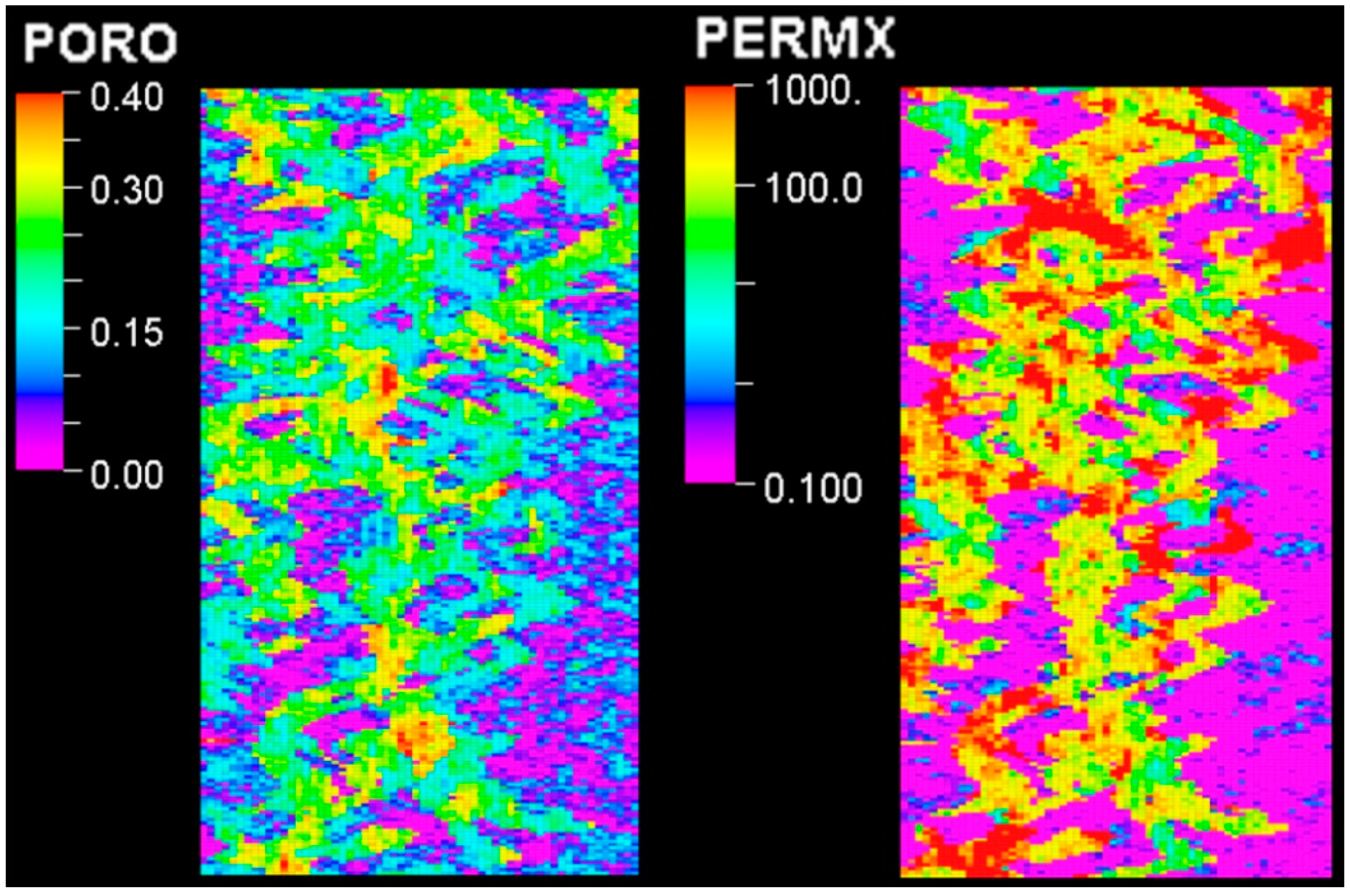
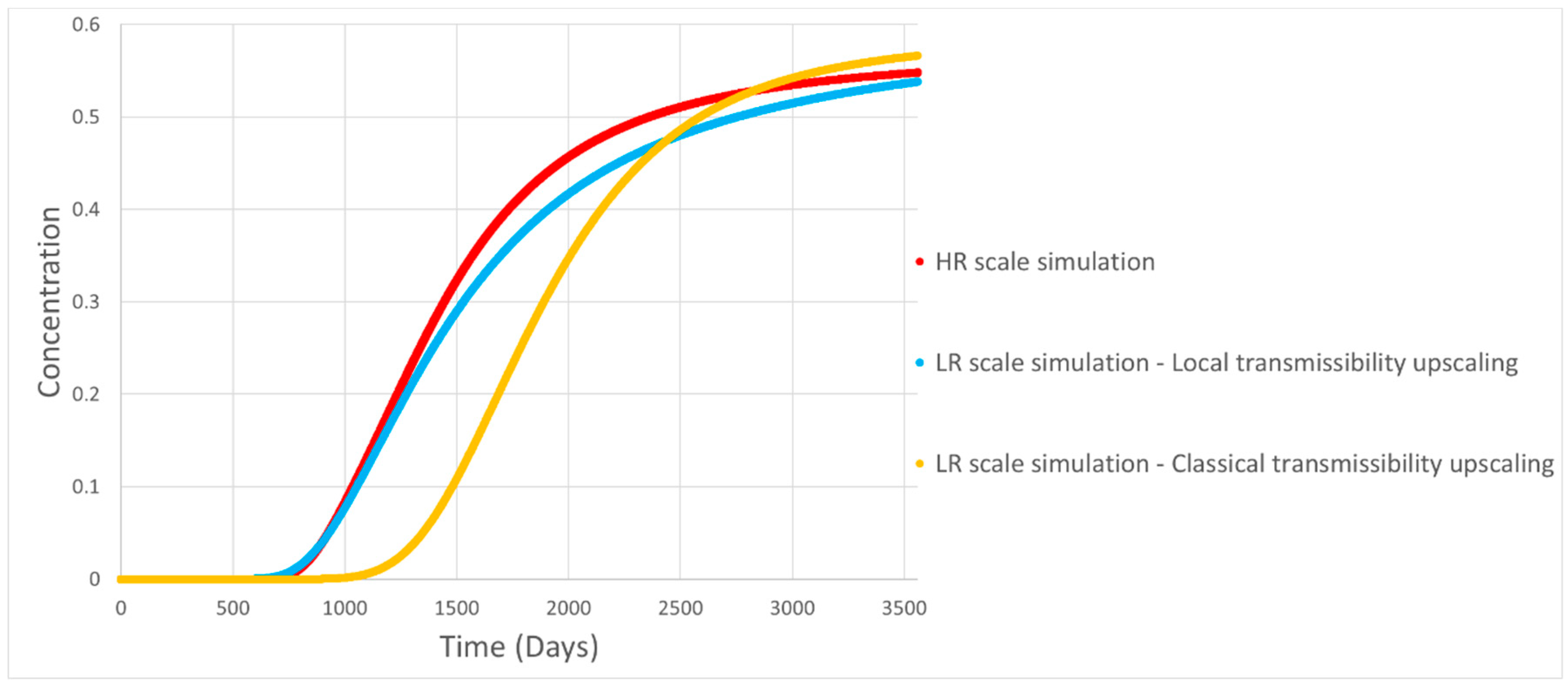
3. Application to the SPE-10 Model

The presented method is applied to a two-dimensional synthetic case corresponding to an extracted layer of the “SPE-10 2nd comparative solution” project [26]. This map corresponding to the 51st layer is located in the lower part (Upper-Ness formation) of the model.

Figure 8 shows the permeability distribution in I and J-direction and the porosity distribution. The range of the permeability varies by 8 orders of magnitude (1.5 × 10⁻³ mD to 2 × 10⁵ mD). The range of the porosity varies from 10⁻³ to 0.4.

One injector well and one producer well are considered. The location of the wells is given in

Table 1. Coordinates of well locations.

Wells	I-Coordinate	J-Coordinate
Injector	3	3
Producer	58	218

. Both wells are vertical with perforation throughout the formation of the reservoir.

The scenario is an eight-year CO₂ injection. The fluid injection rate is equal to 100 m³/day constraints by a maximum Bottom hole pressure at 690 bar. The fluid is produced at a constant bottom hole pressure of 275 bar.

The breakthrough curves obtained with the high-resolution geological scale and large-scale reservoir simulation have been compared. Figure 9 shows that the results of geological high-resolution scale simulation and large-scale reservoir simulation with the local transmissibility upscaling method are similar. The arriving time is the same. The large-scale reservoir simulation with a classical transmissibility upscaling approach based on flow calculation shows an offset on the breakthrough time.

4. Conclusions

Reservoir engineering procedures require the upscaling of geological grid properties to perform reservoir simulations. The upscaling process affects these properties, especially in highly heterogeneous reservoirs.

In this paper, a new approach has been developed to upscale transmissibility values. This method uses the half-block approach and combines the finite volume principles with algebraic methods to provide an upper and a lower bound of the upscaled transmissibility values. The upscaled transmissibility calculation is done considering the half parts of the blocks on each side of the boundaries of the two grid blocks to keep the heterogeneity contrast observed at the high-resolution geological scale. The combination of 1D numerical solutions and algebraic averaging leads to a rapid approach.

In this paper, we have shown on an extracted map of the SPE10 model that:

(1)

This approach is more accurate than classical transmissibility upscaling method based on flow simulation;

(2)

This approach keeps the contrast of transmissibility values observed at the high-resolution geological scale and improves the accuracy of field-scale flow simulation for highly heterogeneous reservoirs;

(3)

The upper and lower bounds delivered by the algebraic method allow checking the quality of the upscaling and the gridding.

In this paper, the problematic of the transmissibility upscaling in fractured reservoirs [27,28,29,30] has not been addressed. An extension of the proposed method will be proposed to upscale the “matrix-fracture” transmissibility values for the dual-continuum models.

References

1. Corvi, P.; Heffer, K.; King, P.; Tyson, S.; Verly, G.; Ehlig-Economides, C.; Le Nir, I.; Ronen, S.; Shultz, P.; Corbett, P.; et al. Reservoir characterization using expert knowledge, data and statistics. Oilfield Rev. 1992, 4, 25–31. [Google Scholar]
2. Sbaï, A.; Amraoui, N. Development and application of diagnostic tools for seawater intrusion analysis in highly heterogeneous coastal aquifers. In E3S Web of Conferences; EDP Sciences: Ullis, France, 2018; Volume 54. [Google Scholar]
3. Mansoori, J. A Review of Basic Upscaling Procedures: Advantages and Disadvantages; The American Association of Petroleum Geologists: Tulsa, OK, USA, 1994; pp. 65–74. [Google Scholar]
4. Kumar, A.; Noh, M.H.; Ozah, R.C.; Pope, G.A.; Bryant, S.L.; Sepehrnoori, K.; Lake, L.W. Reservoir simulation of CO2 storage in aquifers. SPE J. 2005, 10, 336–348. [Google Scholar] [CrossRef]
5. Liang, Y.; Wen, B.; Hesse, M.A.; DiCarlo, D. Effect of dispersion on solutal convection in porous media. Geophys. Res. Lett. 2018, 45, 9690–9698. [Google Scholar] [CrossRef]
6. Christie, M.A. Upscaling for Reservoir Simulation; Society of Petroleum Engineers: St. John’s, NL, Canada, 1996. [Google Scholar] [CrossRef]
7. Renard, Ph.; De Marsily, G. Calculating equivalent permeability: A review. Adv. Water Resour. 1997, 20, 253–278. [Google Scholar] [CrossRef] [Green Version]
8. Durlofsky, J. Upscaling of geocellular models for reservoir flow simulation: A review of recent progress. In Proceedings of the 7th International Forum on Reservoir Simulation Bühl, Baden-Baden, Germany, 12–27 June 2003. [Google Scholar]
9. Nœtinger, B.; Vincent, A.; Ghassem, Z. The future of stochastic and upscaling methods in hydrogeology. Hydrogeol. J. 2005, 13, 184–201. [Google Scholar] [CrossRef]
10. King, P.R. The use of renormalization for calculating effective permeability. Transp. Porous Media 1989, 4, 37–58. [Google Scholar] [CrossRef]
11. Guérillot, D.; Rudkiewicz, J.L.; Ravenne, C.; Renard, G.; Galli, A. An integrated model for computer aided reservoir description: From outcrop study to fluid flow simulations. Revue de l’Institut français du pétrole 1990, 45, 71–77. [Google Scholar] [CrossRef]
12. Gallouët, T.; Guérillot, D. An optimal method for averaging the absolute permeability. In Proceedings of the International Reservoir Characterization Technical Conference, Tulsa, OK, USA, 3–5 November 1991. [Google Scholar]
13. Gallouët, T.; Guérillot, D. Averaged Heterogeneous Porous Media by Minimisation of the Error on the Flow Rate. In Proceedings of the ECMOR IV—4th European Conference on the Mathematics of Oil Recovery, Roros, Norway, 7–10 June 1994. [Google Scholar]
14. Terpolilli, P.; Hontans, T. Boundary effects in the upscaling of absolute permeability–A new approach. In Proceedings of the ECMOR VII—7th European Conference on the Mathematics of Oil Recovery, Baveno, Italy, 5–8 September 2000. [Google Scholar]
15. Samier, P. A Finite Element Method for Calculating Transmissibilities in N-point Difference Equations using a Non-Diagonal Permeability Tensor. In Proceedings of the ECMOR II—2nd European Conference on the Mathematics of Oil Recovery, Arles, France, 11–14 September 1990. [Google Scholar]
16. Ding, Y.; Urgelli, D. Upscaling of transmissibility for field scale flow simulation in heterogeneous media. In Proceedings of the Proceedings of the SPE Symposium on Reservoir Simulation, Dallas, TX, USA, 8–11 June 1997. [Google Scholar]
17. Urgelli, D. Upscaling of Transmissibility Applied to Corner Point Geometry; Society of Petroleum Engineers: St. John’s, NL, Canada, 1998. [Google Scholar] [CrossRef]
18. Wang, W.; Gupta, A. Transmissibility Scale-up In Reservoir Simulation; Petroleum Society of Canada: St. John’s, NL, Canada, 1999. [Google Scholar] [CrossRef]
19. Panfili, P.; Cominelli, A.; Calabrese, M.; Albertini, C.; Savitskiy, A.; Leoni, G. Advanced upscaling for Kashagan reservoir modeling. SPE Reserv. Eval. Eng. 2012, 15, 150–164. [Google Scholar] [CrossRef]
20. Albertini, M.; Prisco, M.; Villa, F.; Kolyubaeva, O.; Stefanucci, M. High-Resolution Reservoir Simulator and Transmissibility Upscaling as a Key to Reservoir Modelling Optimization in an Extra-Heavy Oil Field. Proccedings of the Offshore Mediterranean Conference, Ravenna, Italy, 29–31 March 2017. [Google Scholar]
21. Qi, D.; Hesketh, T. Quantitative Evaluation of Information Loss in Reservoir Upscaling; Society of Petroleum Engineers: St. John’s, NL, Canada, 2004. [Google Scholar] [CrossRef]
22. Sablok, R.; Aziz, K. Upscaling and Discretization Errors in Reservoir Simulation; Society of Petroleum Engineers: St. John’s, NL, Canada, 2005. [Google Scholar] [CrossRef]
23. Ganjeh-Ghazvini, M.; Masihi, M.; Baghalha, M. Study of heterogeneity loss in upscaling of geological maps by introducing a cluster-based heterogeneity number. Phys. A Stat. Mech. Appl. 2015, 436, 1–13. [Google Scholar] [CrossRef]
24. Preux, C. About the use of quality indicators to reduce information loss when performing upscaling. Oil Gas Sci. Technol.–Revue d’IFP Energies nouvelles. 2016, 71, 7. [Google Scholar] [CrossRef] [Green Version]
25. Preux, C.; Le Ravalec, M.; Enchéry, G. Selecting an appropriate upscaled reservoir model based on connectivity analysis. Oil Gas Sci. Technol.–Revue d’IFP Energies nouvelles 2016, 71, 60. [Google Scholar] [CrossRef] [Green Version]
26. Christie, M.A.; Blunt, M.J. Tenth SPE Comparative Solution Project: A Comparison of Upscaling Techniques; Society of Petroleum Engineers: St. John’s, NL, Canada, 2001. [Google Scholar]
27. Kfoury, M.; Ababou, R.; Noetinger, B.; Quintard, M. Upscaling fractured heterogeneous media: Permeability and mass exchange coefficient. J. Appl. Mech. 2006, 73, 41–46. [Google Scholar] [CrossRef]
28. Vitel, S.; Souche, L. Unstructured upgridding and transmissibility upscaling for preferential flow paths in 3D fractured reservoirs. In SPE Reservoir Simulation Symposium; Society of Petroleum Engineers: St. John’s, NL, Canada, 2007. [Google Scholar] [CrossRef]
29. Lemonnier, P.; Bernard, B. Simulation of naturally fractured reservoirs. state of the art-part 1–physical mechanisms and simulator formulation. Oil Gas Sci. Technol.–Revue de l’Institut Français du Pétrole 2010, 65, 239–262. [Google Scholar] [CrossRef] [Green Version]
30. Lemonnier, P.; Bourbiaux, B. Simulation of naturally fractured reservoirs. state of the art-Part 2–matrix-fracture transfers and typical features of numerical studies. Oil Gas Sci. Technol.–Revue de l’Institut Français du Pétrole 2010, 65, 263–286. [Google Scholar] [CrossRef] [Green Version]
Figure 1. A two dimensional in space (2D) illustration of the sampling method. (left) Large reservoir cells; (right) high-resolution geological cells associated with each large reservoir cell.
Water 11 02647 g001
Figure 2. A two dimensional (2D) illustration of the cell domains: left (blue) and right (yellow) or north (orange) and south (green).
Water 11 02647 g002
Figure 3. Transmissibility calculation.
Water 11 02647 g003
Figure 4. A two dimensional (2D) illustration of the half transmissibility calculation of the (right) local part of the cell A (yellow) and the (left) local part of the cell B (blue) for the lower bound transmissibility.
Water 11 02647 g004
Figure 5. A two dimensional (2D) illustration of the lower estimated bound value for the transmissibility between two large reservoir cells. Red arrows represent the half transmissibility of the right domain of the left cell (yellow) and the half transmissibility of left domain of the right cell (blue).
Water 11 02647 g005
Figure 6. A two dimensional (2D) illustration of the half transmissibility calculation of the (right) local domain of the cell A (yellow) and the (left) local domain of the cell B (blue) for the upper bound transmissibility.
Water 11 02647 g006
Figure 7. A two dimensional (2D) illustration of the upper estimated bound value for the transmissibility between two large reservoir cells. Red arrows represent the half transmissibility of the right domain of the left cell (yellow) and the half transmissibility of the left domain of the right cell (blue).
Water 11 02647 g007
Figure 8. Permeability (I and J) (log scale) and porosity distribution of the 51st layer of the SPE10 model.
Water 11 02647 g008
Figure 9. Comparisons of breakthrough curves for the production well.
Water 11 02647 g009