Article

Feasibility of Multi-Year Forecast for the Colorado River Water Supply: Time Series Modeling

1
Department of Mathematics and Statistics, Utah State University, Logan, UT 84322, USA
2
Utah Climate Center/Department of Plants, Soils & Climate, Utah State University, Logan, UT 84322, USA
3
State of Colorado’s Colorado River Representative, Denver, CO 80202, USA
4
Squire Patton Boggs, LLP., Denver, CO 80202, USA
5
Central Weather Bureau, Taipei 100, Taiwan
*
Author to whom correspondence should be addressed.
Water 2019, 11(12), 2433; https://doi.org/10.3390/w11122433
Submission received: 27 August 2019 / Revised: 7 November 2019 / Accepted: 14 November 2019 / Published: 20 November 2019

Abstract

:
The future of the Colorado River water supply (WS) affects millions of people and the US economy. A recent study suggested a cross-basin correlation between the Colorado River and its neighboring Great Salt Lake (GSL). Following that study, the feasibility of using the previously developed multi-year prediction of the GSL water level to forecast the Colorado River WS was tested. Time-series models were developed to predict the changes in WS out to 10 years. Regressive methods and the GSL water level data were used for the depiction of decadal variability of the Colorado River WS. Various time-series models suggest a decline in the 10-year averaged WS since 2013 before starting to increase around 2020. Comparison between this WS prediction and the WS projection published in a 2012 government report (derived from climate models) reveals a widened imbalance between supply and demand by 2020, a tendency that is confirmed by updated WS observation. Such information could aid in management decision-making in the face of near-future water shortages.

Graphical Abstract

1. Introduction

The Colorado River is one of the largest water resources in the United States, supplying water to about 40 million people in the southeast and intermountain states. As recently reported by the Colorado River Research Group (2018) [1], water supply of the Colorado River (hereafter “WS”) has decreased in recent decades, while the river basins are facing the biggest drought in recorded history. In terms of climatic conditions, the decrease in WS is largely attributed to increasing temperatures that led to less snow and more water being evaporated than normal (Barnett et al. 2008, McCabe et al. 2007, Udall et al. 2017) [2,3,4]. However, the long-term future of the WS made by climate model projections showed an upturn in the Colorado River WS into 2020 (BOR 2012) [5]; this is in contradiction to an observed decrease through 2018. Notwithstanding future water supply projections, (BOR 2012) [5] anticipates water demand to surpass supply by as much as 3.2 million acre feet through 2050. Such growing imbalance between supply and demand requires a more accurate and longer-term predictions of the Colorado River WS given projected water demand.
Western water managers are concerned about multiyear droughts, even more so than for a single dry year, since the shifts between persistently dry and wet regimes have important implications for managing the limited water resources (Gangopadhyay et al. 2010) [6]. Multi-year drought is reflected in the pronounced quasi decadal oscillation of 10–20 years featured in the Colorado River WS’s historical record, as noted by a recent study (Wang et al., 2018) [7]; however, this low-frequency feature is unaccounted for by the climate model projections published in the government report (BOR 2012) [5]. The neighboring watershed of the Upper Colorado River Basin—the Great Salt Lake (GSL) of Utah—also shows a marked low-frequency variability in its water level variation (Lall et. al. 1995, Wang et al. 2010) [8,9]. The GSL water level variation is coherent with the low-frequency variation of the Colorado River WS (Wang et al. 2018) [7]. Meanwhile, past studies (Gillies et al. 2015, Gillies et al. 2011) [10,11] have developed time series modeling to anticipate the GSL water level out to 5–10 years. Predictability of streamflow and water storage at decadal timescale was reported elsewhere, such as the Missouri River basin (Neri et al. 2018; Wang et al. 2014) [12,13]. Therefore, a compelling case can be made that the same multi-year forecast developed for the GSL water level could apply to the Colorado River WS.
Given the challenges in anticipating the near-term (decadal) variation of the Colorado River WS imposed by climate models, given their lack of or inconsistent decadal climate variations (BOR, 2012) [5], an empirical prediction model for the Colorado River WS offers a provisional solution. The goal, therefore, was to explore the role of the aforementioned decadal-scale climate oscillations and their interconnection to water supply for the near future, beyond seasonal streamflow prediction. The concept is to examine multi-year predictability in water supply by conducting time series modeling that uses observational data of the GSL water level and the Colorado River WS. The work presented here does not analyze the mean-state hydroclimate changes toward the end of the century, which has already been done (Barnett et al. 2008) [2], nor does it apply climate indices to enhance seasonal prediction for the Colorado River WS. To this end, data and the time series modeling are introduced in Section 2. Results and validation of the two modeling approaches are presented in Section 2.2 and Section 2.3, respectively. Discussion of the results, the physical explanation, and the implications are offered in Section 3. Section 4 provides some concluding remarks.

2. Materials and Methods

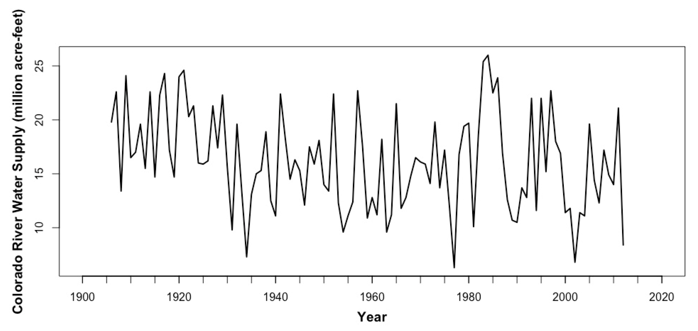
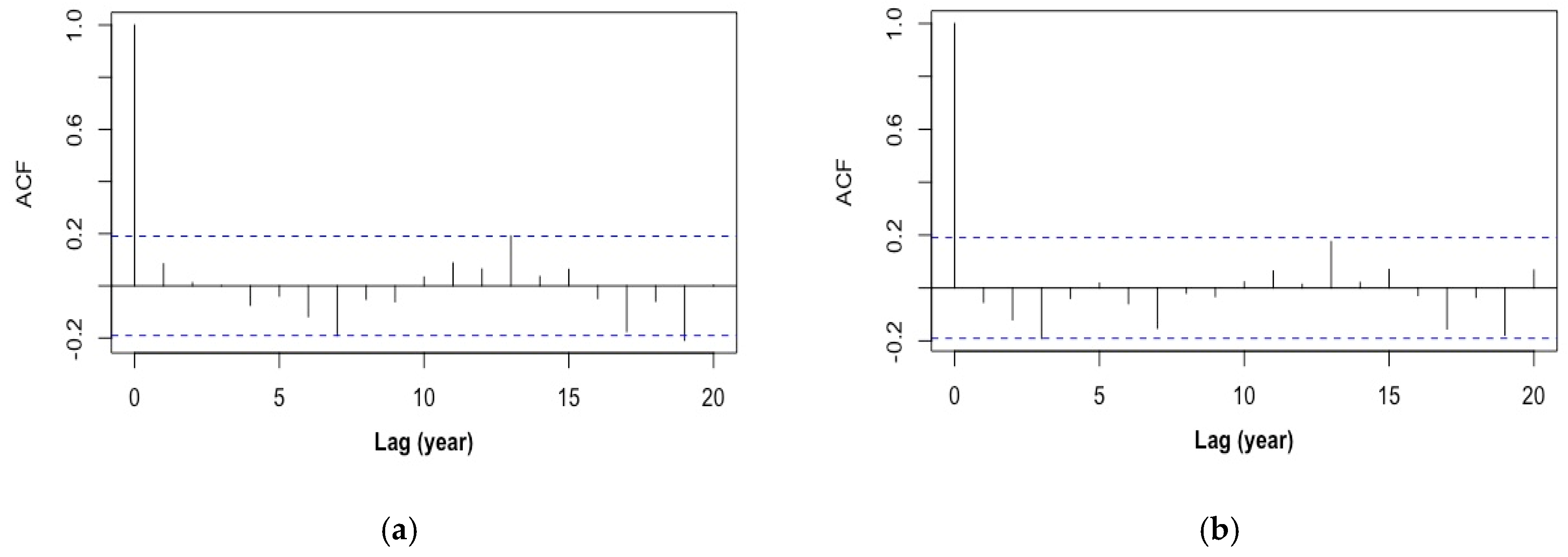
2.1. Data and Methodology

We used the annual Colorado River Water Supply data from the Bureau of Reclamation (BOR) study from 1906 to 2012 and subjected it to a backward 10-year moving average (as was done in the BOR report). The GSL water level data was obtained from the US Geological Survey up to June 2016. Figure 1 shows the observed time series of the annual Colorado River WS data from 1906 to 2012. The time series does not appear stationary since the mean seems to fluctuate. In order to fit a time series model, the raw data needs to be transformed into a stationary series with a time-invariant mean and covariance, which is typically achieved by differencing. Let W t denote the raw WS data. The first-order differencing is defined as
X t = W t W t 1 .
The resulting difference series X t , i.e., the annual WS anomaly, is input into the subsequent time series analysis. Notice that we skipped the first observation due to the differencing, so X t has a total of 106 observations. After the analysis is complete, the differencing will be undone to make predictions for the actual W t .
To get a first impression of the correlation structure of X t , the autocorrelation function (ACF) and the partial autocorrelation function (PACF) of X t were computed (Figure 2). There appear to be a few significant lags, in the ACF at lag 1 and in the PACF at lags 1 and 2. The correlations at lags 13 and 19 are marginally significant in the ACF, and so is the correlation at lag 12 in the PACF. These significant lags suggest that an autocorrelation structure in the WS data is present, one that can be utilized to build univariate time series models, such as the autoregressive moving-average (ARMA) (p, q), for predicting WS based on its own historical observations. Here, the numbers p and q denote the autoregressive and moving-average orders, respectively. Readers are referred to, e.g., (Brockwell et al. 2002) [14] for the mathematical details.
In time series analysis, the cross-autocorrelation function (CACF), or simply the cross-correlation function, between two time series, is the correlation between values of the processes at different times (Brockwell et al. 1991) [15]. It is an important measure of independence between time series. Significant values in the CACF indicate certain correlations of the underlying series. The CACF of the first-order difference, i.e., annual anomalies, of the Colorado River WS and the Great Salt Lake (GSL) water level is shown in Figure 3. There is a significant cross-autocorrelation at lag −1, which leads us to use the GSL time series as an exogenous variable to further improve the univariate model. This approach gave us an ARMAX (p, q, w, s) model, which stands for an ARMA (p, q) model with exogenous variables (Cryer and Chan 2008) [16]. Here, the numbers w and s denote the autoregressive and moving-average orders of the linear filter for the exogenous variables, respectively.
In the following sections, we will present in detail each of the ensuing models and their fit to the WS data. To simplify notations, hereafter, the differenced Colorado River WS time series is denoted by X t and the exogenous GSL time series is denoted by S t .

2.2. Univariate Time Series Models

The autocorrelation structure of X t as shown in Figure 2 seems to suggest a simple ARMA model such as moving average and MA (1) and auto-regressive AR (2). We tried both models and the mean squared errors (MSE’s) were 20.24 and 23.37, respectively. Compared to the unconditional variance 32.25, these two models have explained about 37% and 27% of the total variability, respectively. The ACF’s of the residuals of the two models are plotted in Figure 4. In principle, the residual should resemble white noise, i.e., a time series that exhibits no autocorrelations, to indicate sufficiency of the underlying model. Both residuals shown in Figure 4 are close to being white noise, but still with a few marginally significant autocorrelations, e.g., at lags 7, 13, 17, and 19 for MA (1) and at lags 3 and 19 for AR (2). This means that both models are close to but not perfectly fit.

2.2.1. ARMA (1, 1)

To improve on fitting, we ran a systematic search of low-order ARMA models, but none of them could completely remove all the autocorrelations. Among these, ARMA (1,1) is the simplest yet reasonably effective model with an in-sample MSE of 19.98. We thus chose it as one candidate model. The estimated model equation is
X t =   0.094 + 0.1264 X t 1 + Z t 0.9026 Z t 1
where Z t is a white-noise process with an estimated variance of 19.98. Figure 5 shows three diagnosis plots of this model. Notice that there are still a couple of marginally significant autocorrelations (e.g., at lag 13 and 19) as shown in the ACF plot. In fact, lag 19 shows up significant since it is an important variable for the WS series. This leads us to consider a long-order autoregressive (AR) model that includes lag 19 in the following.

2.2.2. Sparse AR (19)

AR process is known to have great flexibility that can answer many questions both in theory and applications of time series analysis (Akaike 1969) [17]. However, very often in practice, in order for an AR process to achieve satisfactory performances, it must allow for a relatively large order. For example, in our case, the order must be at least 19, which means there has to be at least 19 variables in the model. This can be problematic in the situation when a more parsimonious model is desired. A common solution is to keep the important lags and remove redundant ones, leading to a sparse AR model, referred to as SAR hereafter. There have been extensive studies of SAR models in the literature, especially with regard to model selection and parameters estimation (Sang and Sun 2015) [18]. The goal is to achieve the desired flexibility while keeping the AR model as simple as possible. In our analysis here, after a systematic search, the best SAR (19) model chosen included lags 1–12, as well as 17 and 19. The fitted model equation is
X t = 0.7693 0.7636 X t 1 0.6914 X t 2 0.6046 X t 3 0.4989 X t 4 0.4858 X t 5 0.4033 X t 6 0.5391 X t 7 0.45 X t 8 0.4607 X t 9 0.3942 X t 10 0.251 X t 11 0.2472 X t 12 0.1348 X t 17 0.2287 X t 19 + Z t ,
where Z t represents a white-noise process with an estimated variance of 16.47. The residual plot and its ACF are shown in Figure 6, along with the plot of model fitted values and the 95% confidence intervals versus the observed. Notice that the residuals resemble a white noise with no significant autocorrelations, which indicates the sufficiency of the model.

2.3. ARMA Models with Exogenous Variables

2.3.1. SARX (19, 1, 0)

The first ARMAX model selected is SARX (19, 1, 0), meaning that the differenced WS data X t has an SAR (19) fitted as the base model, and additionally the differenced GSL data S t and its first lag as the exogenous variables. The model equation is estimated to be
X t =   0.83   ( S t 0.9897 S t 1 ) 0.9139 0.7854 X t 1 0.7249 X t 2 0.6983 X t 3 0.5695 X t 4 0.6024 X t 5 0.4777 X t 6 0.7116 X t 7 0.5629 X t 8 0.6026 X t 9 0.5099 X t 10 0.3829 X t 11 0.3028 X t 12 0.1566 X t 17 0.2655 X t 19 + Z t
and the estimated variance of the white noise is improved to 14.27. Figure 7 displays the three diagnosis plots of this model.

2.3.2. ARMAX (19, 1, 2, 0)

The second ARMAX model selected is ARMAX (19, 1, 2, 0). It fits an ARMA (19, 1) to X t as the base model and adds S t and its first two lags as exogeneous variables. The estimated model is
X t =   1.3673   ( S t 1.2105 S t 1 0.9484 S t 2 ) x x x 0.5633 X t 1 0.4935 X t 2 0.5659 X t 3 0.4735 X t 4 0.4148 X t 5 0.4217 X t 6 0.6114 X t 7 0.4178 X t 8 0.4981 X t 9 0.3982 X t 10 0.2857 X t 11 0.2691 X t 12 0.098 X t 17 0.227 X t 19 0.3073 Z t 1 + Z t ,
and the estimated variance of white noise is further reduced to 13.22. The diagnosis plots of this model are shown in Figure 8.

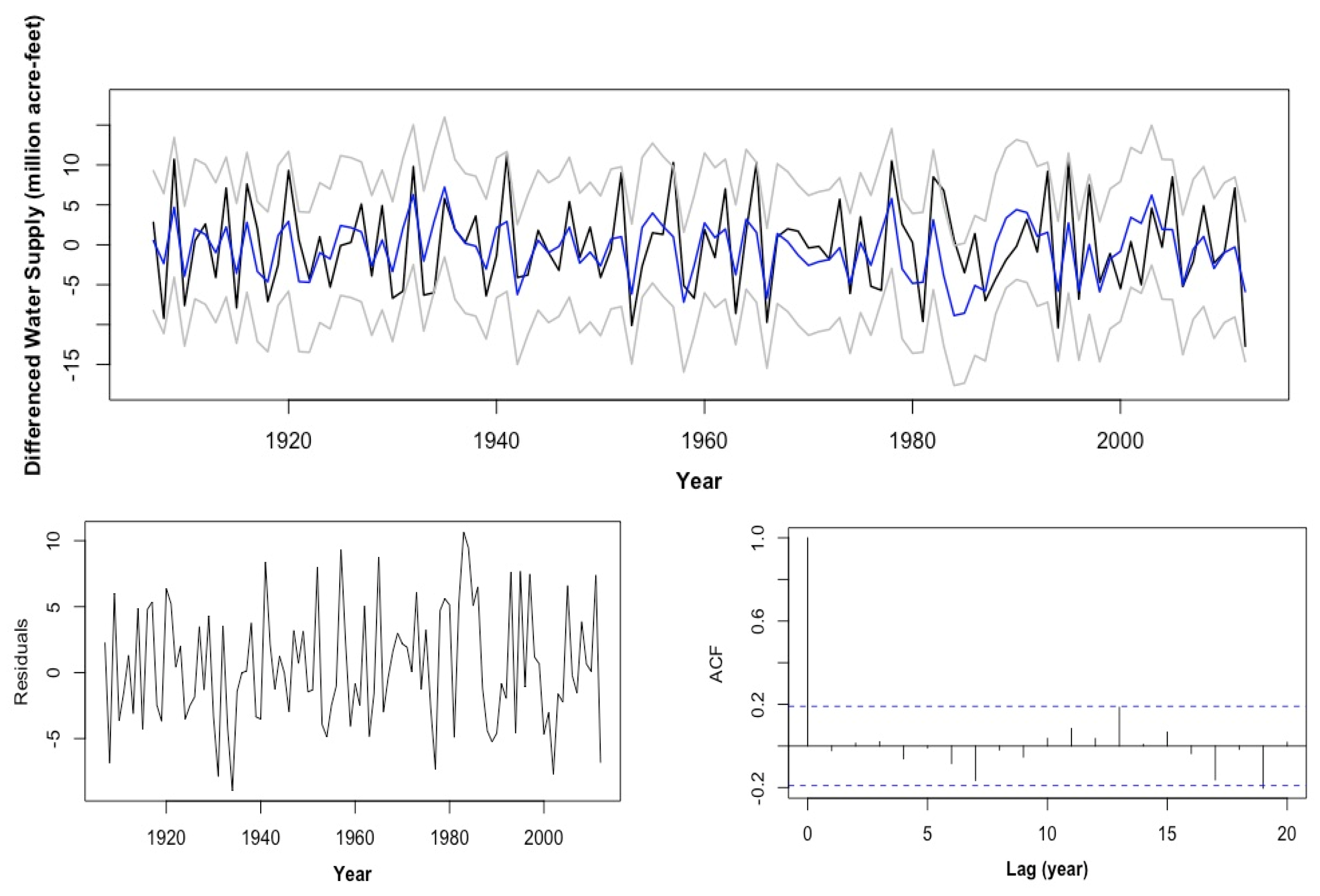
2.4. Cross-Validation

Next, cross-validation was performed to assess the forecasts of the models. For a typical time-series analysis, the standard strategy for cross-validation is to split the data by 90%/10% or 80%/20%. However, the precondition for doing so is having sufficient amount of data. In this case, the data is extremely limited considering the complexity of the models, with only 106 observations. In terms of statistical information, we have to keep the training data as large as possible, otherwise the estimation becomes unstable and the cross-validation is not meaningful. Since our goal here is to test the forecastibiliy of five years ahead, we chose the validation set to have only five observations.
The differenced WS data X t was divided into a training and a test set, with the first 101 observations being the training set while the last five observations being the test data. We used 10 forecasting horizons (h = 1, 2, …, 10, i.e., length of the forecast) and the coefficients of the model were updated at every step. For h = 1, (one-step ahead prediction), the model was fitted on observations 1–101 to predict observation 102, and then the model was fitted using observations 1–102 to predict observation 103, and so on. For h = 2, (two-step ahead prediction) the model was fitted using observations 1–100 to predict observation 102, then the model was fitted using observations 1–101 to predict observation 103, and so on. The results of the ten forecasting horizons are shown in Table 1, along with the corresponding root mean squared error (RMSE) and the skill score (Murphy 1988) [19] of each model. To simplify notations, here in Table 1, we use the acronyms “ARMA,” “SAR,” “SARX,” and “ARMAX” to represent the ARMA (1, 1), SAR (19), SARX (19, 1, 0), and ARMAX (19, 1, 2, 0) models, respectively.
The ARMA (1,1) model apparently does not quite capture the dynamics of the WS data. It practically only has one-year-ahead predicting power. As we can see from Table 1, from h = 2 on, its prediction is almost the same as the constant model, i.e., the unconditional mean. This confirms our previous finding that lag 19 is an essential variable for forecasting the WS series, and thus, any effective model has to inevitably account for this complexity.
Among the rest three models, the SAR (19) model has the lowest RMSE for one-step-ahead prediction and three-step-ahead prediction. For h = 2, 4, 5 and 6, the SARX (19, 1, 0) model is the best. This model also has the lowest forecasting error when h = 10. For h = 7 to 9, the model with the lowest RMSE is ARMAX (19, 1, 2, 0). Numerical details of these results are shown in Table 1. The skill score as a one-to-one correspondence of the RMSE shows the consistent results.
In conclusion of the cross-validation presented here, the best model appears to be SARX (19, 1, 0), as this model can achieve the forecasting horizons up to six years.

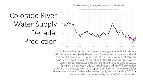
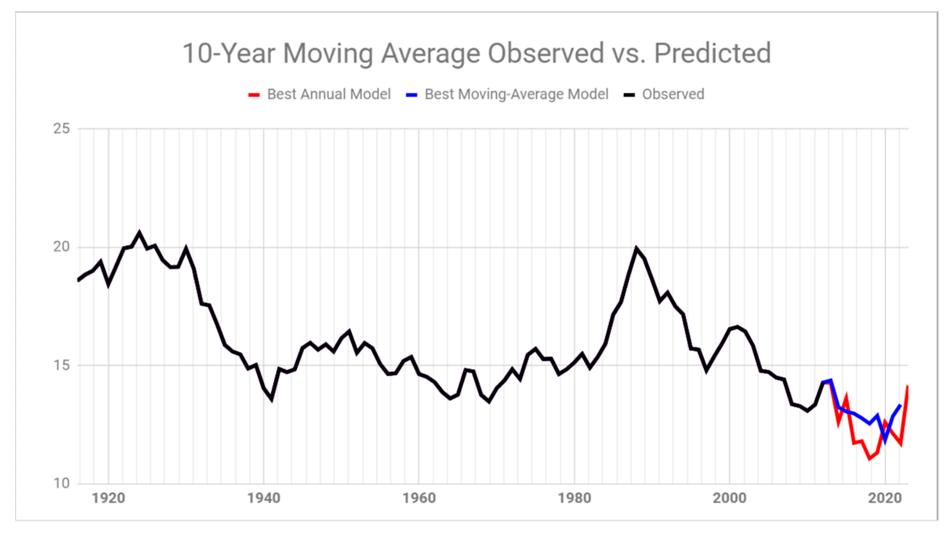
2.5. Benchmark Modeling Using the 10-Year Moving-Average Data

In the government study of (BOR 2012) [5], the WS data was presented in the form of the (backward) 10-year moving average in order to highlight its marked decadal-scale variability. Thus, it is prudent to conduct a similar time series analysis using the 10-year moving average of both the Colorado River WS and the Great Salt Lake water level. Below is a general formula that was used to create the moving average.
W ˜ t = i   =   0 9 W t i 10 ,   for   t = 10 ,   11 ,   12 ,
where W ˜ t is the new 10-year moving-average time series and W t represents the raw annual WS data. The 10-year moving-average of the GSL data was similarly created. Note that the first 9 observations of each data set were removed. Figure 9 shows the time series of these 10-year moving-average WS and GSL. The GSL time series is very smooth due to the large and shallow lake minimizing the interannual variability and thereby enhancing the low frequency, climate-driven variations (Lall and Mann 1995, Wang et al. 2010, 2012) [8,9,20]. Again, first-order differencing was applied to these moving-average data to achieve stationarity. The resulting differenced moving-average series for WS and GSL are denoted by X ˜ t and S ˜ t , respectively. The final models selected are
  • Ten-Year Moving-Average Univariate Model AR (19)
    The best univariate model chosen for the 10-year moving-average WS is an AR (19) model; this is consistent with the raw-data model in Section 2.2. The fitted model is
    X ˜ t =   0.1992 X ˜ t 1 0.0514 X ˜ t 2 + 0.1731 X ˜ t 3 + 0.0887 X ˜ t 4 0.0282 X ˜ t 5 + 0.0334 X ˜ t 6   0.1966 X ˜ t 7 + 0.1174 X ˜ t 8 0.0532 X ˜ t 9 0.5161 X ˜ t 10 + 0.1626 X ˜ t 11 0.1017 X ˜ t 12 +   0.3447 X ˜ t 13 +   0.0144 X ˜ t 14 + 0.115 X ˜ t 15 0.1354 X ˜ t 16 0.281 X ˜ t 17 0.0375 X ˜ t 18 0.2447 X ˜ t 19 + Z t ,
    where Z t is a white-noise process with an estimated variance of 0.1946.
  • Ten-Year Moving-Average ARMAX (13, 10, 7, 0)
    One of the ARMAX models chosen had an ARMA (13, 10) base, and it includes 7 GSL elevation lags. The model equation is
    X ˜ t =   0.0493 S ˜ t + 1.772 S ˜ t 1 2.4889 S ˜ t 2 + 1.1278 S ˜ t 3 0.6349 S ˜ t 4 0.4446 S ˜ t 5 + 1.4953 S ˜ t 6 0.7594 S ˜ t 7 + 0.184 X ˜ t 3 + 0.2239 X ˜ t 13 0.6748 Z t 10 + Z t
    where Z t is a white noise process with an estimated variance of 0.2051.
  • Ten-Year Moving-Average ARMAX (19, 10, 7, 0)
    The other competitive ARMAX model for the ten-year moving-average WS also included 7 GSL lags and had an ARMA (19, 10) base. The equation is estimated as
    X ˜ t =   0.0493 S ˜ t + 1.7720 S ˜ t 1 2.4889 S ˜ t 2 + 1.1278 S ˜ t 3 0.6349 S ˜ t 4 0.4446 S ˜ t 5 + 1.4953 S ˜ t 6   0.7594 S ˜ t 7 + 0.1837 X ˜ t 3 +   0.2223 X ˜ t 13 +   0.0153 X ˜ t 18   0.1264 X ˜ t 19 0.6690 Z t 10 + Z t
    where Z t is a white noise process with an estimated variance of 0.2018.
Cross-validation was subsequently applied by dividing the 10-year moving-average WS time series into a training set and a test set. Considering that the moving-average data has lots of overlaps among observations (i.e., any two adjacent observations have nine annual data observations in common in their formations), the split here is slightly different than the annual data. The training set included the first 81 observations, while the test data set included the last 15 observations. This way, the test data set has at least five observations that are independent with the training set. Ten forecasting horizons were used (h =1, 2,…10) as was previously done. The results are shown in Table 2, along with the corresponding RMSE and the skill score of each model. The two ARMAX models had a similar performance in terms of the MSE of fitting, i.e., the estimated white noise variance. More importantly, they significantly outperformed the univariate model in terms of forecasting, as shown in Table 2 (in which the lowest RMSE at each horizon is bold). Table 2 also displays the results of the skill score, where the model with the highest skill score is indicated.
In conclusion of this cross-validation study, the best model for h = 4 and beyond (i.e., forecast out to at least five years) is the ARMAX (19, 10, 7, 0) model.

3. Prediction Results

In this section, we make predictions of water supply for the next 10 years (2013–2022) and discuss the results from both the annual and moving-average models we have developed in the previous section. Figure 10a shows the 10-year prediction and the associated 95% confidence interval for the SAR (19), SARX (19, 1, 0), and ARMAX (19, 1, 2, 0) models that were developed in Section 2 for the annual WS data. Computation of the confidence interval is based on the asymptotic normality of the prediction (Brockwell and Davis 2002) [14]. Despite the cross validations that justify their forecasting performance from statistics viewpoint, the predicted differenced WS in all these models is noisy and the 95% confidence intervals are too large to be practical. In other words, these models are not suitable for predicting individual years’ value. Statistically, this is largely due to the insufficiency of data: 106 observations are too few for models with more than 20 parameters. As more data are available, the predicting power is expected to improve.
To be comparable with the BOR study, i.e., to focus on the low-frequency variation of WS, we display in Figure 11 the 10-year moving-average of WS along with both predictions using the best models of the annual data and ten-year moving average data. The predictions here are shown in terms of their 10-year moving average. Despite the slightly more detailed variations predicted by the annual data model, forecasts of the smoothed WS by both models show an overall decreasing trend in water supply for about seven years and then an increase for the next three. The implication is that the water levels may not be higher than they are now for at least a decade, at least compared to what was previously projected in (BOR 2012) [5]. This predicted widening of the supply-demand imbalance is in agreement with the updated WS data published by the Environmental Defense Fund (Rachel O’Connor 2019) [21]. As of this writing, the Upper Colorado River snowpack hovers slightly above average (e.g., the 18 February 2019 BOR data puts the Upper Colorado River Basin headwaters at 110% of the historic average). This inferred current condition may seem contradictory to the downtrend predicted in Figure 11, but again, the present prediction depicts the 10-year MA, and it should not be a quantitative indication for any individual year.

4. Discussion

The different time lags linking the Colorado River WS and the GSL water level reflect the hydrologic buffering shared by the two basins (Wang et al. 2018) [7], since a majority fraction of the surface water is contributed by groundwater. (Fang and Shen 2017) [22] showed that the annual streamflow-storage correlation in this region is medium-high, depicting a high baseflow fraction that normally leads to a high annual correlation between streamflow-storage correlation. As a result, the GSL water level and the low-frequency variation of the Colorado River WS are highly coherent (Wang et al. 2018) [7]; this, in turn, enables the former to be a predictor for the latter, a previously undocumented feature that is examined in this study. Compared to the seasonal statistical water supply forecasts for the Western US (Pagano et al. 2009) [23], which uses the Z-score regression and has been in operation, the work presented here employs time series forecasting to predict the multi-year tendency (instead of individual years’ value).
The various time lags adopted in the models present somewhat different physical meanings. For instance, the 19-year lag in GSL appears to echo the documented multi-decadal variability associated with the Interdecadal Pacific Oscillation of ~35 years (i.e., 1/2 cycle) (Dai 2012, Wang et al. 2012) [20,24]. Likewise, the three-year and six-year lags in GSL are coincident with a quarter-phase and half-phase of the energetic ~12-year cycle, respectively, that characterizes the Great Basin precipitation (Smith et al. 2015, Wang et al. 2009) [25,26]. Previous time-series modeling in predicting the GSL level by (Gillies et al. 2015, 2011) [10,11] have pointed out similar connections with the notable climate cycles in this region. These results are in line with previous finding by (Switanek and Troch 2011) [27] that it is possible to forecast Colorado River streamflow at the decadal timescale by using ocean-atmosphere teleconnections. Future, Leher et al. (2017) [28] pointed out that decadal precipitation trends may be causing the persistent prediction errors for spring and summer runoff, a trend the present forecast is trying to capture.
The prediction presented here is not without caveats and one potential problem is in the use of a moving average in the predictand (i.e., the WS) and the predictor (the GSL); this is because a MA operator can alter the time structure. When interpreting the forecast of these moving-average model(s), there could be missing information at the interannual timescale making the year-by-year validation impractical. Meanwhile, the GSL undergoes considerable diversions leading to a long-term decline in its water level (Bedford 2009, Mohammed and Tarboton 2012) [29,30]. Quantification of the GSL diversions is difficult due to the complexity of the Bear River that runs through three states prior to entry into the GSL, as well as the effect of groundwater withdrawal that reduces recharge to the lake (Hakala 2014, Masbruch et al. 2016) [31,32]. While GSL diversions create a slow, monotonic downward trend in the lake level, such a trend produces autocorrelation and thereby should be corrected via the inclusion of autoregressive terms in the model.

5. Conclusions

The outcome of this study highlights the need to reexamine the water supply of the Colorado River called for by (Ayres et al. 2016) [33]. The temporal coherence between the low-frequency variations of the Colorado River and GSL storage systems (Wang et al. 2018) [7] provides the basis for the time series modeling undertaken here. The models were used to assess the forecast potential and the results point to the feasibility of using the GSL water level to assist in the forecast of the Colorado River WS, beyond seasonal timescales. Predictions by these models were compared in terms of annual data versus 10-year moving averages. The predictive potential of the GSL elevation, as was demonstrated in previous studies, is one of conceivable application and adoption as a forecast method useful for the Colorado River WS, especially in the face of prolonged drought as has been observed in the recent decade.
The 170-year-long record of the GSL water level makes it a useful indicator of the Colorado River WS variation at its decadal frequency (Wang et al. 2018) [7], and the presented analysis demonstrates that decadal predictability may be obtainable through common time-series modeling approaches. The multi-year prediction of the Colorado River (Figure 11) is particularly striking in that it suggests a decrease through 2020 rather than an increase as shown in (BOR 2012) [5]. In other words, the prediction implies a widened imbalance between supply and demand by as much as 2.5 million acre feet (maf) in 2060; this imbalance, if verified, would be considerably greater than the 2012 estimation of the BOR study. While water-saving plans can be tailored more to scenarios where water supplies decrease further in the future, this paper presents statistical prediction of WS that can be useful in the implementation of these plans. We conclude that Colorado River managers would be pragmatic to periodically assess future WS through the adaptation of a decadal prediction approach.

Author Contributions

B.P. and Y.S. designed the methods and wrote the manuscript. S.-Y.S.W. and R.R.G. designed the project and edited the manuscript. J.E. and C.-C.W. edited the manuscript and improved the presentation.

Funding

This study is supported by the Bureau of Reclamation WaterSMART program under Award Number R18AC0018, the US Department of Energy, Office of Biological and Environmental Research program under Award Number DE-SC0016605, and the USU Agriculture Experiment Station under #9264.

Acknowledgments

The authors thank the three anonymous reviewers for their constructive comments and the graphical assistance by Kegan Black.

Conflicts of Interest

The authors declare no conflict of interest.

References

  1. Colorado River Research Group. It’s Hard to Fill a Bathtub when the Drain is Wide Open: The Case of Lake PowellRep; CRRG: Boulder, CO, USA, 2018. [Google Scholar]
  2. Barnett, T.P.; Pierce, D.W. When will Lake Mead go dry? Water Resour. Res. 2008, 44, W03201. [Google Scholar] [CrossRef]
  3. McCabe, G.J.; Wolock, D.M. Warming may create substantial water supply shortages in the Colorado River basin. Geophys. Res. Lett. 2007, 34. [Google Scholar] [CrossRef]
  4. Udall, B.; Overpeck, J. The twenty-first century Colorado River hot drought and implications for the future. Water Resour. Res. 2017, 53, 2404–2418. [Google Scholar] [CrossRef]
  5. BOR. Colorado River Basin Water Supply and Demand Study; BOR: Washington, DC, USA, 2012; p. 34. [Google Scholar]
  6. Gangopadhyay, S.; McCabe, G.J. Predicting regime shifts in flow of the Colorado River. Geophys. Res. Lett. 2010, 37. [Google Scholar] [CrossRef]
  7. Wang, S.-Y.; Gillies, R.R.; Chung, O.-Y.; Shen, C. Cross-Basin Decadal Climate Regime Connecting the Colorado River with the Great Salt Lake. J. Hydrometeorol. 2018, 19, 659–665. [Google Scholar] [CrossRef]
  8. Lall, U.; Mann, M.E. The Great Salt Lake: A barometer of low-frequency climatic variability. Water Resour. Res. 1995, 31, 2503–2515. [Google Scholar] [CrossRef]
  9. Wang, S.-Y.; Gillies, R.R.; Jin, J.; Hipps, L.E. Coherence between the Great Salt Lake Level and the Pacific Quasi-Decadal Oscillation. J. Clim. 2010, 23, 2161–2177. [Google Scholar] [CrossRef]
  10. Gillies, R.R.; Chung, O.Y.; Wang, S.Y.S.; DeRose, R.J.; Sun, Y. Added value from 576 years of tree-ring records in the prediction of the Great Salt Lake level. J. Hydrol. 2015, 529, 962–968. [Google Scholar] [CrossRef]
  11. Gillies, R.R.; Chung, O.Y.; Wang, S.Y.S.; DeRose, R.J.; Sun, Y. Incorporation of Pacific SSTs in a time series model towards a longer-term forecast for the Great Salt Lake elevation. J. Hydrometeorol. 2011, 12, 474–480. [Google Scholar] [CrossRef]
  12. Neri, A.; Villarini, G.; Salvi, K.A.; Slater, L.J.; Napolitano, F. On the decadal predictability of the frequency of flood events across the US Midwest. Int. J. Climatol. 2019, 39, 1796–1804. [Google Scholar] [CrossRef]
  13. Wang, S.Y.; Hakala, K.; Gillies, R.R.; Capehart, W.J. The Pacific quasi-decadal oscillation (QDO): An important precursor toward anticipating major flood events in the Missouri River Basin? Geophys. Res. Lett. 2014, 41, 991–997. [Google Scholar] [CrossRef]
  14. Brockwell, P.; Davis, R.A. Introduction to Time Series and Forecasting, 2nd ed.; Springer: Berlin, Germany, 2002. [Google Scholar]
  15. Brockwell, P.; Davis, R.A. Time Series: Theory and Methods, 2nd ed.; Springer: Berlin, Germany, 1991. [Google Scholar]
  16. Cryer, J.D.; Chan, K.S. Time Series Analysis with Applications in R, 2nd ed.; Springer: Berlin, Germany, 2008. [Google Scholar]
  17. Akaike, H. Fitting autoregressive models for prediction. Ann. Inst. Stat. Math. 1969, 21, 243–247. [Google Scholar] [CrossRef]
  18. Sang, H.; Sun, Y. Simultaneous sparse model selection and coefficient estimation for heavy-tailed autoregressive processes. Statistics 2015, 49, 187–208. [Google Scholar] [CrossRef]
  19. Murphy, A.H. Skill scores based on the mean squared error and their relationships to the correlation coefficient. Mon. Weather Rev. 1988, 116, 2417–2424. [Google Scholar] [CrossRef]
  20. Wang, S.-Y.; Gillies, R.R.; Reichler, T. Multi-decadal drought cycles in the Great Basin recorded by the Great Salt Lake: Modulation from a transition-phase teleconnection. J. Clim. 2012, 25, 1711–1721. [Google Scholar] [CrossRef]
  21. O’Connor, R. Colorado River Basin Story Map Highlights Importance of Managing Water below the Ground. Available online: http://blogs.edf.org/growingreturns/2019/10/24/colorado-river-basin-story-map-highlights-importance-of-managing-water-below-the-ground/ (accessed on 24 October 2019).
  22. Fang, K.; Shen, C. Full-flow-regime storage-streamflow correlation patterns provide insights into hydrologic functioning over the continental US. Water Resour. Res. 2017, 53, 7499–8314. [Google Scholar] [CrossRef]
  23. Pagano, T.C.; Garen, D.C.; Perkins, T.R.; Pasteris, P.A. Daily Updating of Operational Statistical Seasonal Water Supply Forecasts for the Western US. JAWRA J. Am. Water Resour. Assoc. 2009, 45, 767–778. [Google Scholar] [CrossRef]
  24. Dai, A. The influence of the Inter-decadal Pacific Oscillation on US precipitation during 1923–2010. Clim. Dyn. 2012, 41, 633–646. [Google Scholar] [CrossRef]
  25. Smith, K.; Strong, C.; Wang, S.-Y. Connectivity between historical Great Basin precipitation and Pacific Ocean variability: A CMIP5 model evaluation. J. Clim. 2015, 28, 6096–6112. [Google Scholar] [CrossRef]
  26. Wang, S.-Y.; Gillies, R.R.; Jin, J.; Hipps, L.E. Recent rainfall cycle in the Intermountain Region as a quadrature amplitude modulation from the Pacific decadal oscillation. Geophys. Res. Lett. 2009, 36, L02705. [Google Scholar] [CrossRef]
  27. Switanek, M.B.; Troch, P.A. Decadal prediction of Colorado River streamflow anomalies using ocean-atmosphere teleconnections. Geophys. Res. Lett. 2011, 38. [Google Scholar] [CrossRef]
  28. Lehner, F.; Wood, A.W.; Llewellyn, D.; Blatchford, D.B.; Goodbody, A.G.; Pappenberger, F. Mitigating the impacts of climate nonstationarity on seasonal streamflow predictability in the US southwest. Geophys. Res. Lett. 2017, 44, 12–208. [Google Scholar] [CrossRef]
  29. Bedford, D. The Great Salt Lake America’s Aral Sea? Environ. Sci. Policy Sustain. Dev. 2009, 51, 8–21. [Google Scholar] [CrossRef]
  30. Mohammed, I.N.; Tarboton, D.G. An examination of the sensitivity of the Great Salt Lake to changes in inputs. Water Resour. Res. 2012, 48. [Google Scholar] [CrossRef]
  31. Hakala, K. Climate Forcings on Groundwater Variations in Utah and the Great Basin. Master’s Thesis, Utah State University, Logan, UT, USA, 2014. [Google Scholar]
  32. Masbruch, M.D.; Rumsey, C.A.; Gangopadhyay, S.; Susong, D.D.; Pruitt, T. Analyses of infrequent (quasi-decadal) large groundwater recharge events in the northern Great Basin: Their importance for groundwater availability, use, and management. Water Resour. Res. 2016, 52, 7819–7836. [Google Scholar] [CrossRef]
  33. Ayers, J.; Ficklin, D.L.; Stewart, I.T.; Strunk, M. Comparison of CMIP3 and CMIP5 projected hydrologic conditions over the Upper Colorado River Basin. Int. J. Climatol. 2016, 36, 3807–3818. [Google Scholar] [CrossRef] [Green Version]
Figure 1. The annual basin-wide water supply (WS) data of the Colorado River from 1906 to 2012.
Water 11 02433 g001
Figure 2. (a) The autocorrelation function (ACF) and (b) partial autocorrelation function (PACF) of the first-order difference of the Colorado River WS time series. The two blue dashed lines on each plot denote the corresponding 95% confidence interval.
Water 11 02433 g002
Figure 3. The cross-autocorrelation function (CACF) of the differenced Colorado River and Great Salt Lake (GSL) series. Note the significant cross-autocorrelation at lag −1. The two blue dashed lines denote the 95% confidence interval.
Water 11 02433 g003
Figure 4. Autocorrelation function (ACF) plots of model residuals for (a) MA (1) and (b) AR (2). Blue dashed lines denote the 95% confidence intervals.
Water 11 02433 g004
Figure 5. Diagnosis plots of the ARMA (1,1) model: (top) overlaid plot of the observed annual water supply anomaly X t (black), model fitted value (blue) and its 95% confidence interval (grey); (left) residual plot; (right) ACF of the residual.
Water 11 02433 g005
Figure 6. Diagnosis plots of the SAR (19) model: (top) overlaid plot of the observed annual water supply anomaly X t (black), model fitted value (blue) and its 95% confidence interval (grey); (left) residual plot; (right) ACF of the residual.
Water 11 02433 g006
Figure 7. Diagnosis plots of the SARX (19,1,0) model: (top) overlaid plot of the observed annual water supply anomaly X t (black), model fitted value (blue) and its 95% confidence interval (grey); (left) residual plot; (right) ACF of the residual.
Water 11 02433 g007
Figure 8. Diagnosis plots of the ARMAX (19,1,2,0) model: (top) overlaid plot of the observed annual water supply anomaly X t (black), model fitted value (blue) and its 95% confidence interval (grey); (left) residual plot; (right) ACF of the residual.
Water 11 02433 g008
Figure 9. Plot of the 10-year moving-average water supply in million acre feet (maf) of the Colorado River (a) and plot of the ten-year moving average of Great Salt Lake water level (b).
Water 11 02433 g009
Figure 10. Plot of the observed values (black) with the predictions (red) ten years out for (A) SAR (19) model, (B) SARX (19, 1, 0) model, and (C) ARMAX (19, 1, 2, 0) model in million acre feet (maf). The gray shaded area denotes the 95% predicting confidence interval.
Water 11 02433 g010
Figure 11. The observed values for the 10-year moving average (black) shown with the predictions (red) 10 years out for the best annual model and the predictions (blue) 10 years out for the best moving-average model.
Water 11 02433 g011
Table 1. Cross-validation results for the four models developed for the annual Colorado River Water Supply data. Root mean squared error (RMSE) is shown on top while the skill score (SS) is shown on the bottom. The columns represent the ten forecasting horizons (h = 1, 2, … 10). Highlighted values are the best statistic for each forecasting horizon.
RMSE12345678910
ARMA5.07086.98296.96496.96126.9456.94676.97286.94386.94726.9208
SAR2.86734.48514.53444.3194.18264.10374.3185.12075.26685.2246
SARX3.12744.38094.66464.1573.76973.71164.12955.04215.15735.1757
ARMAX2.8774.39474.97875.17414.05443.99553.73284.48584.91596.2473
SS12345678910
ARMA0.4719−0.0107−0.00800.0029000000
SAR0.83110.5830.57270.61620.63730.6510.61650.45620.42520.4301
SARX0.79910.60220.54790.64440.70540.71450.64930.47270.44890.4407
ARMAX0.830.59970.48490.44910.65920.66920.71340.58270.49930.1852
Table 2. Cross-validation results for the three models developed for the 10-year moving average data. Root mean squared error is shown on top while the skill score is shown on the bottom. The columns represent the ten forecasting horizons (h = 1, 2, … 10). Highlighted values are the best statistic for each forecasting horizon.
RMSE12345678910
AR(19)0.55220.53740.5470.48760.50620.48720.48050.49510.50870.4506
ARMAX10.41520.41230.40790.42680.42970.42660.43160.43690.43150.4312
ARMAX20.41530.4190.41250.41970.42080.41810.41850.42310.42430.4265
SS12345678910
AR(19)0.01810.08020.05410.24580.18110.2350.25370.20910.16050.3391
ARMAX10.4450.45850.47390.42210.40990.41350.39770.38410.39590.3949
ARMAX20.44480.44090.46210.44130.4340.43670.43370.42230.4160.4081

