1. Introduction
River discharge is a fundamental element of the hydrologic cycle and water balance [
1,
2,
3]. It plays a leading role in the development of regional water resources and the protection of river ecologies [
4,
5]. There are large ungauged catchments around the world lacking hydrological data. For example, as a typical ungauged catchment, arid and semi-arid zones account for 15% of the global land area, with 14.4% of the world’s population living in these areas [
6]. The harsh environment in these areas makes the establishment of traditional hydrological stations costly and difficult to manage, which is the primary reason for the lack of hydrological data. Further, insufficient data is a common issue when analyzing climate change, dealing with ecological environment management, and guiding social and economic development [
7,
8]. In areas with privileged economic and observation conditions, various medium- and small-sized rivers are rarely considered as suitable for investing in the development of stations and their high input costs. The dilemma of insufficient hydrological data is a hindrance to the assessment and treatment of water resources and formulation of ecological protection strategies.
To summarize the methods and identify the hydrological characteristics in the ungauged basin, International Association of Hydrological Sciences (IASH) carried out the Prediction of Ungauged Basins (PUB) program from 2003 to 2012 [
9]. The PUB program established a set of methods, including a regression method based on statistics [
10,
11,
12], a scalable method for hydrological characteristics that are similar to those in adjoining watersheds [
13], and a physical similarity method for migration of the hydrological factors contributing to watershed characteristics [
14]. Although the PUB program achieved fruitful results, they are mainly a set of experience methods. When using a hydrological model to estimate the discharge in ungauged catchments, measured data is still necessary for vibrating and benchmarking [
15,
16,
17,
18]. Logically, better simulation results require more hydrological data from ungauged catchments, but the regions themselves lack hydrological observations. Therefore, the use of new methods to directly observe hydrological data, such as building a hydrological station, is the key to resolving this issue [
19,
20,
21,
22].
Remote sensing has been widely used to calculate river discharges in ungauged catchments [
23,
24]. The multi-station hydraulic geometry method supported by Landsat data was used in the Mississippi and Danube rivers [
25], the island area–discharge relationship was fitted in the Yangtze river through satellite data [
21], and hydraulic characteristics of the Yarlung Zangbo River were obtained by remote sensing [
26]. Well-known large rivers of the world are the study areas where remote sensing has been used to estimate discharge. It is difficult to estimate the flow of the widely existing medium- and small-sized rivers. Therefore, new data and methods are required for discharge estimation in medium- and small-sized rivers.
Compared with satellite data, unmanned aerial vehicle (UAV) data has certain advantages in terms of data accuracy [
27,
28,
29]. UAV has been widely used to extract land surface information and river topographic parameters. In aerial photography, spatial data and plane data are collected with the help of UAV [
30]. Moreover, detailed analysis of the elevation is possible using digital models of plant growth established using UAV [
31]. UAV data is an important basis for discharge estimation; it is used to obtain information regarding the underlying hydrological surface. Specifically, in ecological discharge estimations, UAV data is used to calculate the ecological water demand based on gathering information such as the section area of the river, length of the wet perimeter, and depth of the water surface [
32]. In the development of river terraces, UAV remote sensing is used to analyze the changes in river terraces with high-precision data. It is also used to examine the effects of water erosion and transportation on river terraces in plain rivers [
33]. These previous studies supplied many approaches for using UAV to obtain land surface information and river discharge. However, because only a few methods can combine UAV data and hydrological formulae, there are few methods using UAV to directly calculate river discharges in ungauged catchments.
The slope–area method, which was first proposed by Riggs, is a classical hydraulic equation combining geographical and hydraulic factors [
34]. In this theory, the slope of the river, cross-sectional area, and channel roughness can be associated with discharge. When the channel roughness is a constant, discharge is linked with river slope and cross-sectional area [
34]. The slope–area method, based on physical laws and mathematical deduction, has achieved a series of results in the discharge calculation of medium and small rivers [
35,
36,
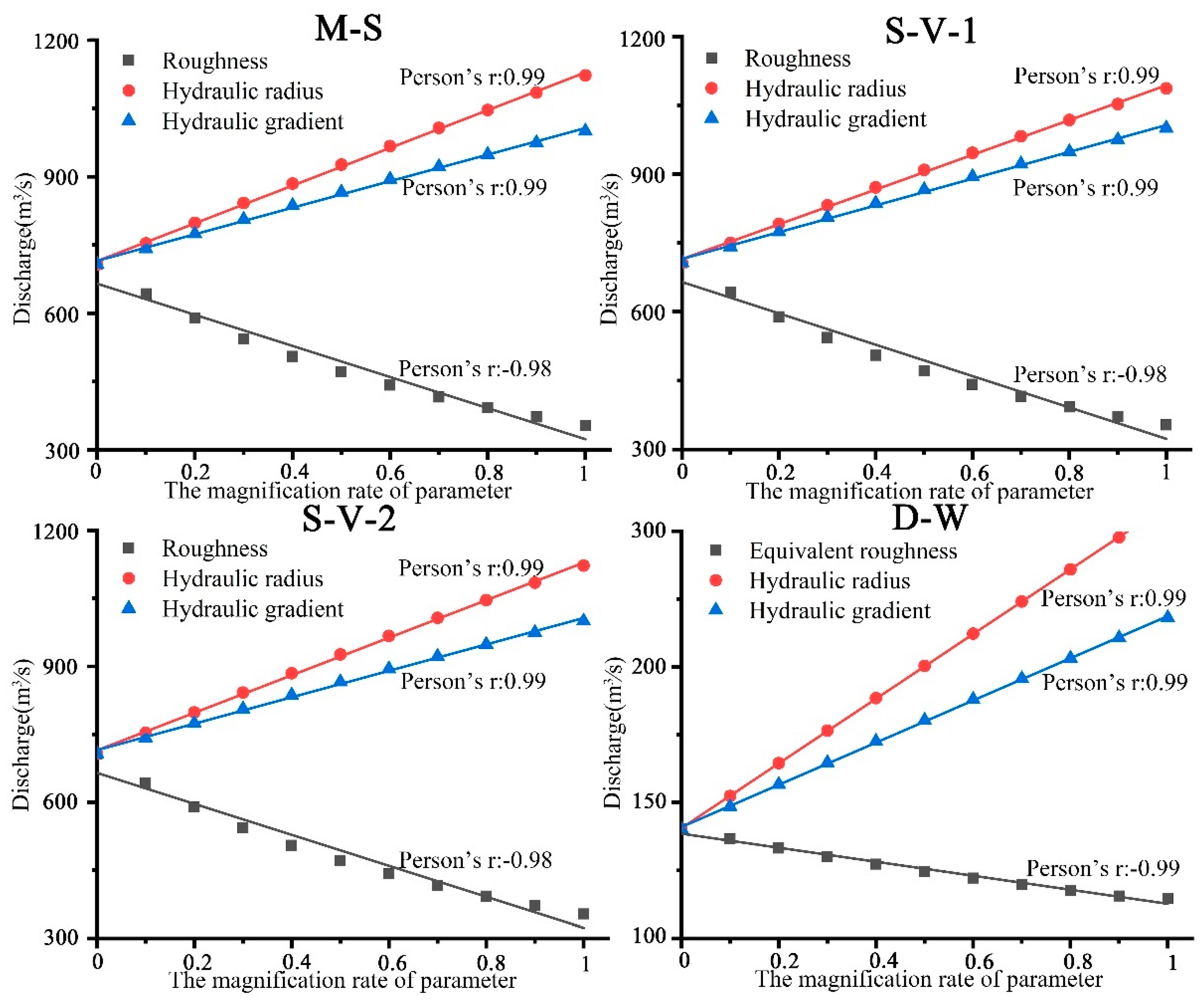
37]. The slope–area method expresses the influence of different environmental factors on river discharge. This method categorized the causes affecting the discharge into geographical factors represented by slope and hydraulic factors represented by river cross-sectional area. Geographical factors represent the impact of the external environment, reflecting the loss of gravitational potential energy, which is caused by the change of terrain. Hydraulic factors represent the impact of the internal environment; the cross-section can control the shape characteristics of water. With different data sources, the slope–area method has various expressions [
37,
38] and has been adapted to complex environments. With the help of multiple data, more methods, such as Manning–Strickler formula (M–S), Saint-Venant system of equivalence (S-V-1, S-V-2), and the Darcy–Weisbach equivalence (D–M) have been applied [
26,
36]. This paper aims to extend the slope–area method using UAV data following three steps:
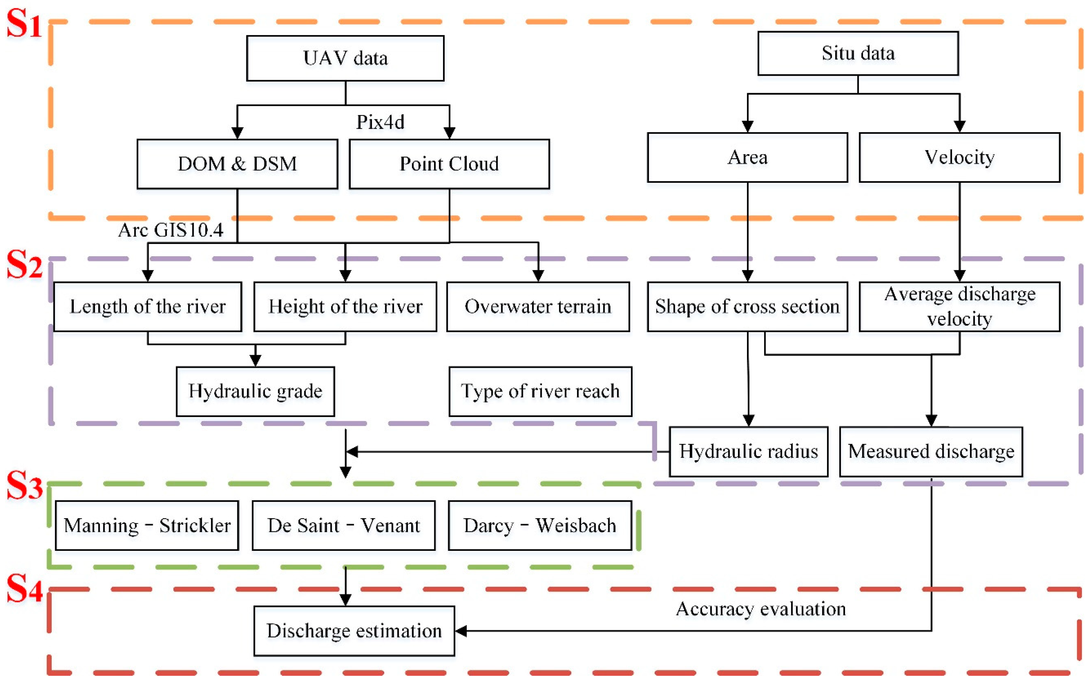
- (1)
UAV is used to acquire terrain data, including the digital surface model (DSM) and digital orthophoto map (DOM), which is the foundation to obtain parameter values;
- (2)
Four classical methods are selected based on slope–area to estimate discharge and calculating the value of parameters;
- (3)
Different methods are evaluated in discharge estimation and the formula that provides the most accurate discharge estimations at different discharge levels is identified.
3. Results
3.1. Preprocessing and Critical Parameter Results
River morphology parameters such as the hydraulic gradient, cross-sectional area, wetted perimeter, and hydraulic radius are necessary for discharge estimation. The vertical section, which shows the variation of elevation with distance, was used to calculate the hydraulic gradient. The area, wetted perimeter, and hydraulic radius were calculated in the cross-section.
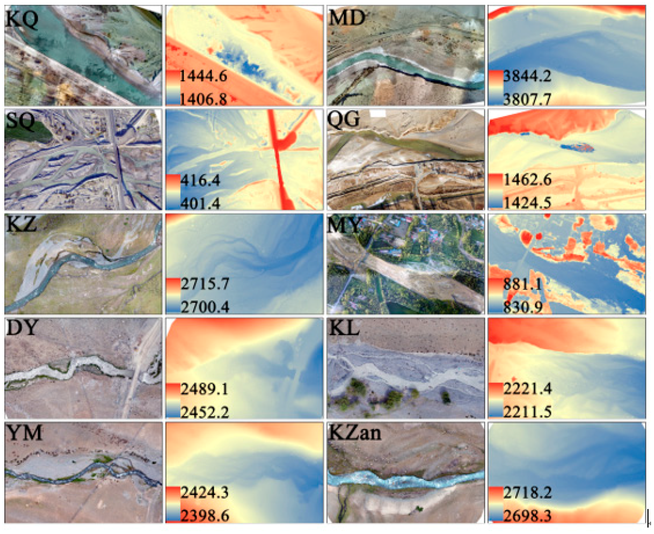
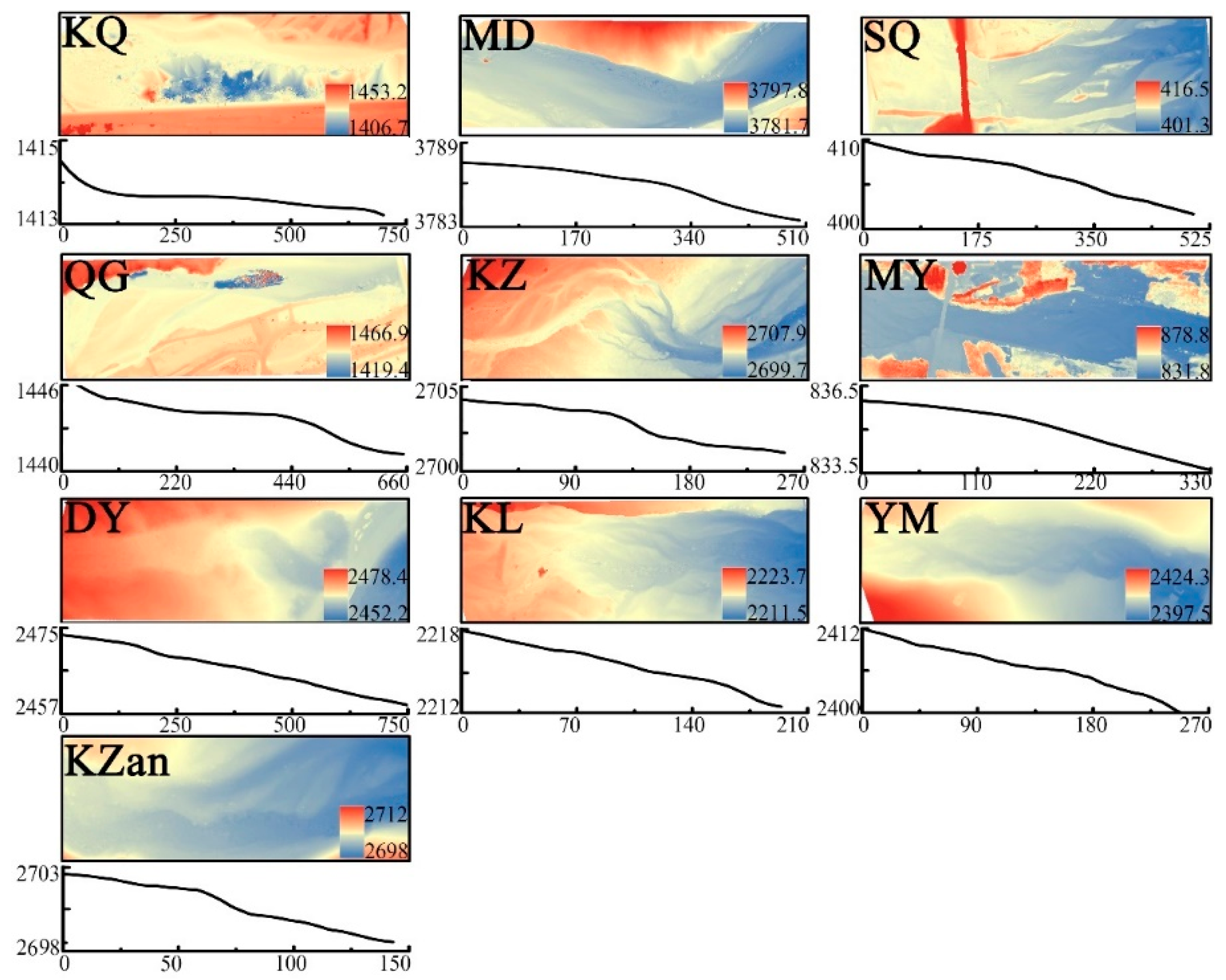
Detailed topographic information and abundant surface information were recorded in the DSM and DOM derived from the UAV images. This information was used to determine the variation of the elevation in the vertical section. The 3D Analyst tool in ArcGIS 10.4 was used to measure minor elevation changes and determine the vertical section of the river.
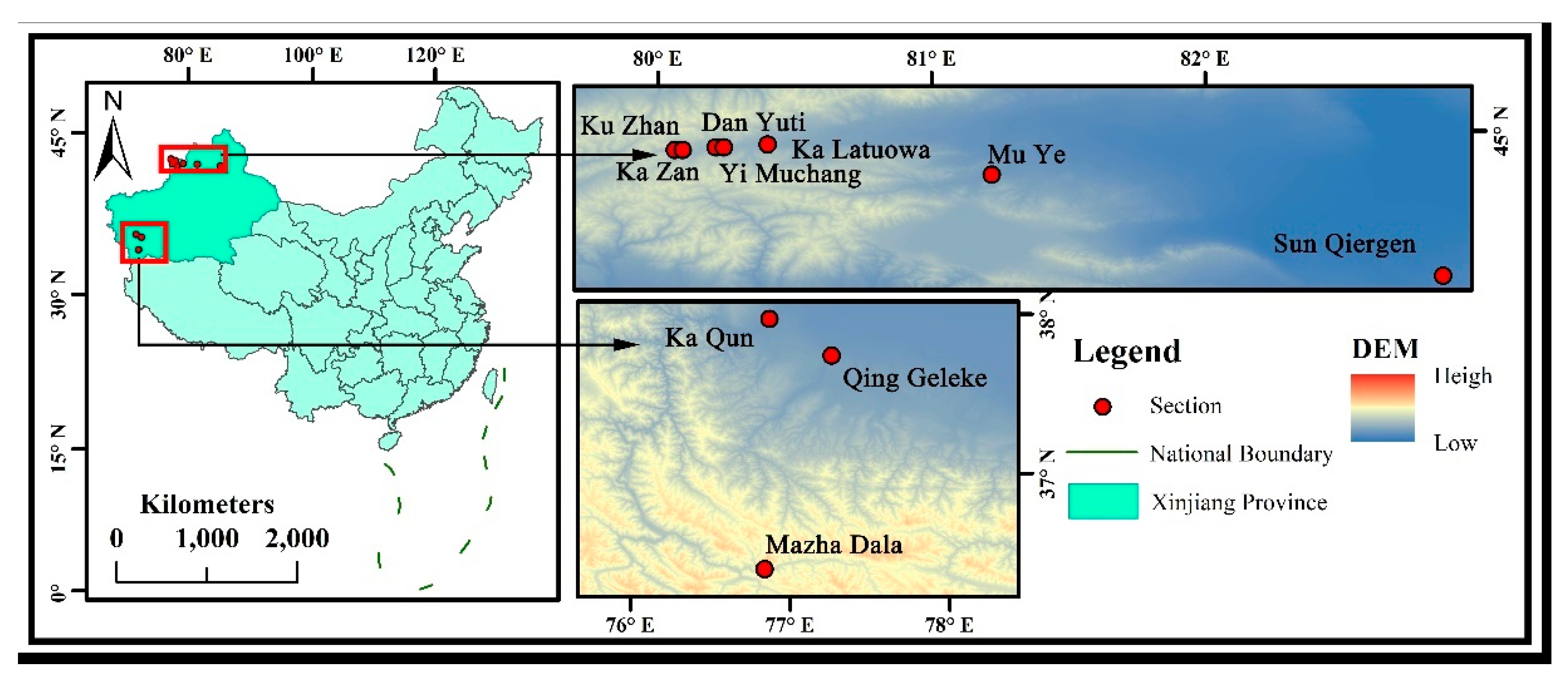
Figure 5 shows the DSM of the study river and the shape of the vertical section. Bridges, roads, and other river-crossing structures appear in the partial study area (SQ, MY, DY, and KL). DSM also recorded their elevation information as interference information for the vertical section. In this study, the width is small relative to the vertical section of the river. When such interferences were encountered, we interrupted the measurement and supplemented the missing part using interpolation. Note that KQ is a concave curve and the others are convex or gentle. The field observations showed that the riverbank of KQ is cement-modified for an agricultural water diversion facility downstream. Only KQ shows evidence of such human management, whereas the other sections exist in their natural state.
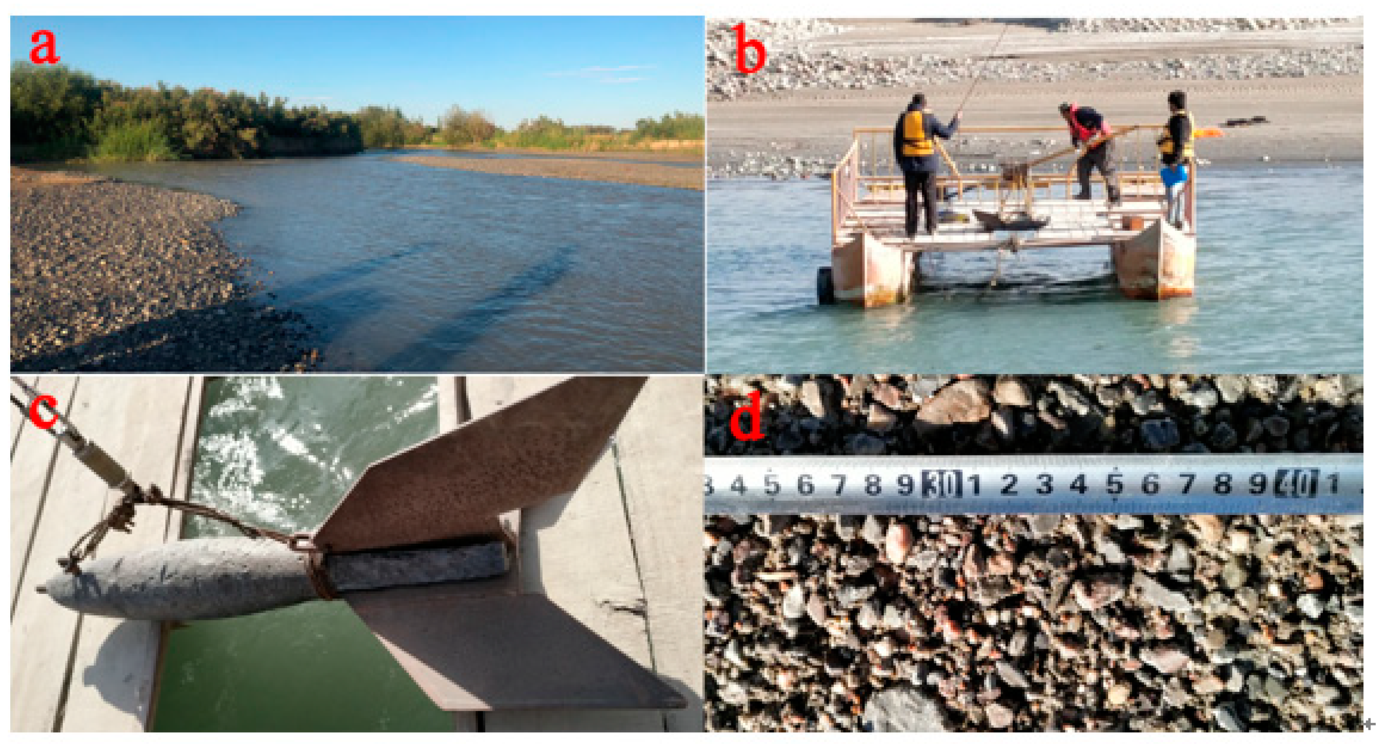
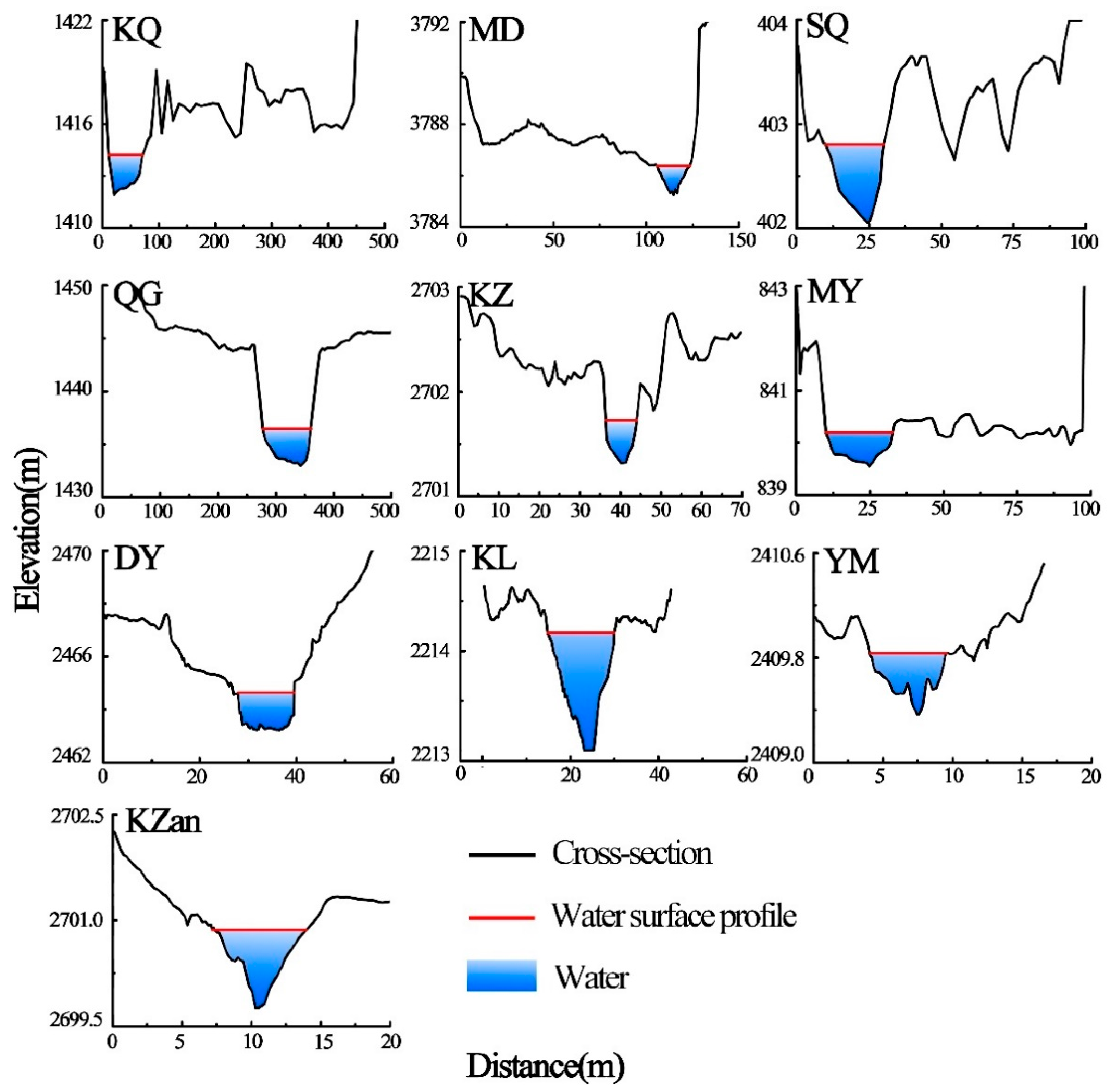
The monitoring section was selected in the middle of the flight area, ensuring that the distance between the upstream and downstream parts was approximately equal. However, the influence of the water body on the elevation measurements cannot be ignored [
49]. The detailed underwater terrain still requires in situ data. We divided the cross-sections into two parts: below the water surface and above the water surface. For the section under the water surface, the terrain data obtained from the UAV were measured manually (
Section 2.2.2). This is particularly helpful in the case of braided rivers and for estimating river-wide discharges (
Figure 6). All sections are triangular or trapezoidal. Some cross-sections are similar to rectangles because of the difference in the ratio of horizontal and vertical coordinates, such as in the QG, KZ, and DY sections. These sections are located in the mountains, where triangles and trapezoids are the normal shapes.
Based on the vertical sections (
Figure 5) and cross-sections (
Figure 6), the hydraulic gradient in the vertical section, the area, and hydraulic radius in the cross-section were computed (
Table 4). These rivers are located in mountainous areas and the parameter values were higher than those for normal rivers. The maximum value of the hydraulic gradient was 0.068 (DY) and the average value was 0.024. Our research targets are medium and small size rivers, which have small cross-sectional areas, triggering the difference in area classification. In all sections, the maximum value was 92.56 m
2 (KQ) and the average was 20.98 m
2. Eight-tenths of the cross-sectional area was less than 20 m
2. The hydraulic radius characterizes the water transport capacity of a section. The sections in this study can be generalized into triangles or trapezoids, and the value of the hydraulic radius is similar to that in narrow-deep rivers.
3.2. Results of the Key Parameters and the River Discharge
The key parameters used in the discharge calculations were obtained from UAV data and in situ experiments (
Table 5). KZan, DY, and YM sections were close to their sources; however, the basin terrain data changes drastically. The values of
J in these sections were relatively larger than others. Because of gravel in KZan, DY, and YM sections, they had the maximum values of roughness (
n) and equivalent roughness (
Δ). Other sections are at the midstream (exit position of the valley) or downstream sections of the river, hence
J was smooth, and
n and
Δ showed medium values. Overall, the parameters of all ten sections were different from those of rivers in the plains.
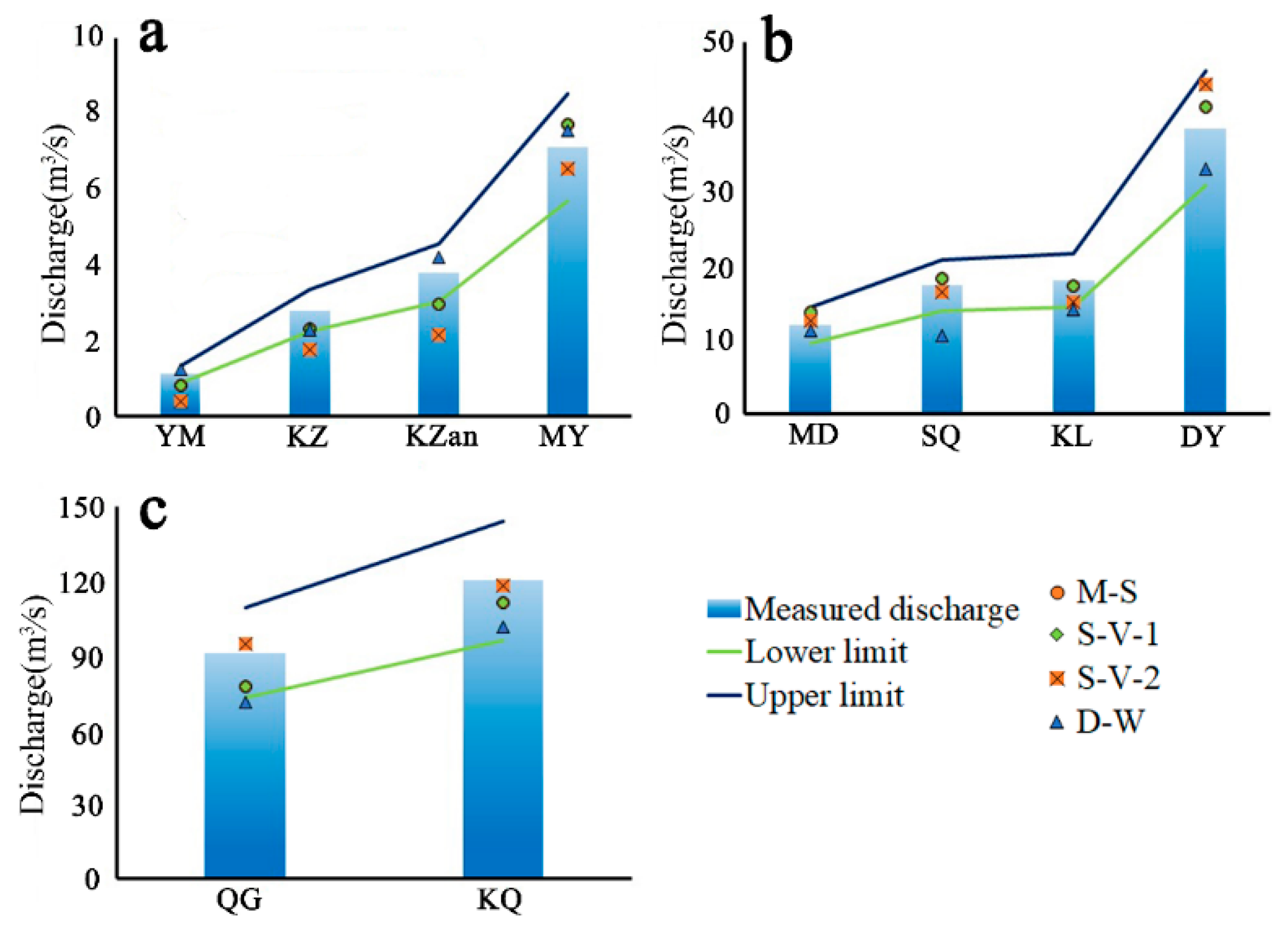
The discharges calculated using M–S, S-V-1, S-V-2, D–W, and the limit of relative accuracy are presented in
Figure 7. To describe the differences, we have divided the results into three parts based on the discharge level: <10 m
3⁄s (
Figure 7a), 10–50 m
3⁄s (
Figure 7b), and >50 m
3⁄s (
Figure 7c). The results given by M–S are consistent with S-V-1 because both M–S and S-V-1 are derived from Chezy’s equation, which is another classical hydrological formula. However, the different equation transformations produce a somewhat different appearance. To illustrate the various calculation methodologies and the complicated relationship among hydrological calculation methods, M–S and S-V-1 are considered as different methods.
3.3. Validation of the Estimated River Discharges
The discharges measured from in situ experiments were regarded as the true values for validating the estimated river discharges. The relative accuracy of M–S, S-V, D–W, and the measured discharge of ten sections are shown in
Figure 7. The overall qualification rate of the discharge calculation method based on UAV data was 70%, with 28 successful calculations and 12 failed calculations. Between these classical methods, when the discharges were greater than 10 m
3⁄s, the D–W method produced an underestimation in KQ, MD, QG, KZan, YM, and SQ sections. Further, when the discharge was greater than 20 m
3⁄s, S-V-2 produced an overestimation in KQ, QG, KZan, and YM sections. M–S and S-V-1 were usually at a medium level. These conclusions were only observed at different discharge levels as different methods have their own characteristics.
Considering the average relative accuracy, the results in all sections are acceptable, except KZ, KZan, and YM. The most significant error was found for the YM section; the average error was 0.35 m3/s, approximately one-third of the measured value. KZ and KZan were in similar situations; their average errors were 0.64 m3/s and 1.11 m3/s, respectively. The measured discharges in KZ, KZan, and YM were less than 5 m3/s. When we set 20% as the evaluation standard, the permitted error was ±1 m3/s, producing a narrow range of acceptable discharges. This is somewhat strict for an empirical formula. The discharge was greater than 5 m3/s in the other seven sections, and the average error in the calculated discharge was within an acceptable limit. Because of the larger margin of error, the calculated discharge varied more widely. For example, in KQ, the measured favorable was 120.33 m3/s and the error in S-V-2 was 1.98 m3/s, which was larger than in KZ, KZan, and YM sections. However, the relative accuracy was 1.64%, the smallest of all the results.
Table 6 shows the NSE of M–S, S-V-1, S-V-2, and D–W. The value of NSE was greater than 0.90 and the average was 0.98. The S-V-2 gave the best NSE value of the four methods. The high values of the NSE meant that calculating river discharge with UAV data was useful. Conventional techniques combined with UAV data have excellent adaptability in the northern Tibet Plateau and Dzungaria Basin.
3.4. Performance of the Methods with Different Discharge Levels
To describe the accuracy of the four methods with respect to the river discharge level, we divided the calculated results into three classes according to the measured discharge. These classes are less than 10 m
3⁄s, 10–50 m
3⁄s, and greater than 50 m
3⁄s, representing low, medium, and high discharges, respectively, in small- and medium-sized rivers (
Table 7). The four methods exhibited different advantages at different discharge levels.
There were four sections where the measured river discharges were less than 10 m
3⁄s (KZ: 2.80 m
3⁄s, KZan: 4.15 m
3⁄s, YM: 1.11 m
3⁄s, and MY: 7.11 m
3⁄s), representing low-discharge rivers. D–W achieved better performance than the other methods (
Figure 7a). The average relative accuracy of the four sections was 9.41%, less than the 20% threshold. Thus, we recommend D–W as the discharge calculation formula for small rivers when the discharge level is less than 10 m
3/s.
Four sections were classified as having a medium discharge level (MD: 15.14 m
3⁄s, DY: 38.44 m
3⁄s, KL: 18.92 m
3⁄s, and SQ: 17.26 m
3⁄s). The M–S and S-V-1 methods offered the best performance for this river class, with an average relative accuracy of 7.95% (
Figure 7b). When the discharge was between 10 m
3⁄s and 50 m
3⁄s, M–S and S-V-1 were better than other methods.
The third discharge level includes KQ (120.33 m
3⁄s) and QG (91.08 m
3⁄s). Compared to the other methods, S-V-2 was the best performer in calculating the discharge of large-flow rivers. The average relative accuracy of S-V-2 for these two sections was 2.74% (
Figure 7c), the calculated results were very close to the measured values.


