A Modified k – ε Turbulence Model for a Wave Breaking Simulation

Abstract

We propose a two-equation turbulence model based on modification of the $k-\epsilon$ standard model, for simulation of a breaking wave. The proposed model is able to adequately simulate the energy dissipation due to the wave breaking and does not require any “a priori” criterion to locate the initial wave breaking point and the region in which the turbulence model has to be activated. In order to numerically simulate the wave propagation from deep water to the shoreline and the wave breaking, we use a model in which vector and tensor quantities are expressed in terms of Cartesian components, where only the vertical coordinate is expressed as a function of a time-dependent curvilinear coordinate that follows the free surface movements. A laboratory test is numerically reproduced with the aim of validating the turbulence modified $k-\epsilon$ model. The numerical results compared with the experimental measurements show that the proposed turbulence model is capable of correctly estimating the energy dissipation induced by the wave breaking, in order to avoid any underestimation of the wave height.

1. Introduction

In the contest of hydraulic engineering, the simulation of hydrodynamic fields, turbulence, and concentration fields of suspended solid particles under wave breaking permits the analysis of the effects produced by the structures on sea bottom and shoreline modifications. The definition of turbulent closure relations under wave breaking is significant in order to adequately represent sediment particle suspension and settling phenomena.

One of the most used approaches is based on depth-averaged motion equations [1,2,3,4], which are obtained by assuming a simplified distribution of the hydrodynamic quantities along the vertical direction (depth-averaged models).

In order to quantify the dissipation mechanism in the surf zone, two strategies are considered in the literature. The first strategy is based on an eddy viscosity approach; in particular, Kazolea and Ricchiuto [5] used a turbulent kinetic energy equation to calculate a breaking viscosity coefficient.

In the context of the second strategy, the extended Boussinesq equations [1,2,3] are used to simulate the propagation of waves in deep water, where dispersive effects are dominant; in the surf zone, the nonlinear shallow water equations are used to simulate shoaling and wave breaking, because the dispersive terms of the Boussinesq equations are switched off. In the surf zone, the nonlinear shallow water equations, integrated by a shock-capturing numerical scheme, are used to simulate the wave breaking, where the nonlinear effects are dominant [4]: the dissipation of the total energy obtained in a shallow water shock is used to implicitly model the energy dissipation due to the breaking. It is evident that it is necessary to introduce a criterion to establish where and when to switch from one system of equations to the other.

In the context defined by the second strategy, the turbulence models are used just in order to determine a distribution of the eddy viscosity coefficient that does not intervene in the simulation of the wave resolving depth-averaged velocity fields but intervene in the simulation of only the concentration fields of suspended solid particles to follow the sea bottom evolution. In this case, the turbulent closure relations that derive from the calculation of the eddy viscosity vertical distribution are carried out by following the line proposed by Fredsøe et al. and Deigaard et al. [6,7] and used by Rakha [8]. In particular, under breaking waves, the instantaneous eddy viscosity vertical distribution is calculated by taking into account the turbulence contribution due to the wave boundary layer and the current and wave breaking [3].

These models are not able to adequately represent the three-dimensional hydrodynamic quantities.

The first three-dimensional models for free surface flows numerically solve the Navier–Stokes equations by adopting the volume of fluid technique (VOF) to track the location of the free surface [9,10]: in the VOF technique, the calculus cells are arbitrarily crossed by the vertical fluxes. Therefore, the pressure and kinematic boundary conditions are not correctly assigned on the free surface.

Another category of models overcomes the above-mentioned difficulty by mapping the physical domain that varies in time along the vertical direction in order to follow the free surface elevation ($\sigma$-coordinate transformation) [11] in a computational domain, which has always a rectangular prismatic shape. In this way it is possible to correctly assign the pressure and kinematic boundary condition on the upper face of the top computational cell [12,13].

These two above-mentioned categories of models empirically introduce, in the surf zone, an appropriate energy dissipation, so that it is possible to represent the decrease of the wave height in the aforementioned zone. Consequently, the location of the initial wave breaking point is settled “a priori”. The definition of the point is where the empirical energy dissipation must be introduced, and therefore the identification of the initial wave breaking point is settled “a priori”.

Shock-capturing methods make it possible to model the energy dissipation due to the breaking by the total energy dissipation obtained in a shallow water shock. The $\sigma$-coordinate shock-capturing methods locate wave breaking without requiring any “a priori” criterion.

In this paper we adopt the new approach proposed by Gallerano et al. [14] in which the motion equations are expressed in terms of variables that are Cartesian based: only the vertical coordinate is expressed as a function of a time-dependent curvilinear coordinate that follows the free surface movements.

In this model the motion equations are numerically solved, on a time dependent curvilinear coordinate system, where the vertical coordinate can vary over time, by using a finite-volume shock-capturing scheme, which uses an approximate HLL (Harten, Lax and van Leer)-type Riemann solver [15].

The shock-capturing scheme [14] does not need to use any “a priori” criterion to identify the location of the initial wave breaking point, and it is able to correctly assign the boundary conditions on the free surface. In this model, by using a computational domain that has a limited number of points along the vertical direction, the numerical wave height fits the experimental measurements before the breaking point and the wave breaking is tracked correctly.

Ma et al. [12] demonstrated that in general the shock-capturing model, defined in the context of the $\sigma$-coordinate, underestimates the energy dissipation at the breaking point and consequently overestimates the wave height in the surf zone.

Therefore, it is necessary to introduce turbulence models that are able to adequately represent the specific energy dissipation at the breaking point.

The definition of turbulent closure relations under wave breaking implies the necessity to consider the production of turbulent kinetic energy associated with the breaking in order to represent sediment particle suspension and settling phenomena.

In order to develop a wave resolving model for nearshore suspended sediment transport, Ma et al. [16] implemented a $k-\epsilon$ model in a three-dimensional $\sigma$-coordinate model to simulate the velocity and particles concentration fields.

In general, $k-\epsilon$ standard models are located in the context of Reynolds-Averaged Navier–Stokes equations (RANS), in which all the unsteady velocity fluctuations are expelled from the simulation of the Reynolds time-averaged velocity fields.

In this approach the effects of all unsteady periodic vortex structures and unsteady stochastic velocity fluctuations are represented in terms of the total transfer of energy dissipation from the averaged motion to all the scales of turbulent motion, through the Reynolds tensor.

In the $k-\epsilon$ standard models, the Reynolds tensor is related to all the energy of the unsteady periodic vortex structures and unsteady stochastic velocity fluctuations that are expelled from the representation of the Reynolds averaged motion. Consequently, these models are not able to directly simulate unsteady periodic vortex structures because they overestimate the Reynolds tensor and produce an excessive dissipation of energy and non-physical wave height reduction.

The velocity field in the surf zone is very complex and is characterized by unsteady periodic vortex structures and unsteady stochastic velocity fluctuations.

Outside the surf zone, the production of turbulent kinetic energy is limited to the oscillating wave boundary layer; inside the surf zone there is the production of turbulent kinetic energy in the oscillating wave boundary layer and the production of turbulent kinetic energy near the wave crest, and between the oscillating wave boundary layer and the wave crest, there is a phenomenon of mainly turbulent kinetic energy dissipation.

In general, the stochastic turbulent fluctuations are superimposed on the periodic unsteady motion of the vortex structures. Bosch and Rodi [17] proposed the simulation of the velocity fields characterized by the above-mentioned unsteady vortex structures by decomposing the instantaneous flow quantities in a time mean component, in a periodic component, and in a turbulent fluctuating component. Following this approach, the sum of the time mean and the periodic part gives rise to the ensemble-average component of the flow quantities. The latter are calculated by the numerical integration of the ensemble-average continuity and momentum equations; the complete spectrum of the stochastic motion is simulated by a statistical turbulence model. The models coherent with the above-mentioned approach are named in the literature as Unsteady Reynolds-Averaged Navier–Stokes (URANS) models.

In this paper, we propose, for the simulation of the wave motion and the turbulence under wave breaking, to expel the turbulent kinetic energy associated with unsteady stochastic velocity fluctuations from the ensemble-average motion. This model can be considered in the context of the Unsteady Reynolds-Averaged Navier–Stokes (URANS) models. The modifications to the $k-\epsilon$ model with respect to the standard one consist of the following:

• The closure relation of the production of turbulent kinetic energy takes into account the nonlinear terms, following the procedure of [18,19];
• The closure relation of the destruction of the dissipation rate is expressed by means of a dynamic procedure, used by Yakhot et al. and Derakty et al. [20,21];
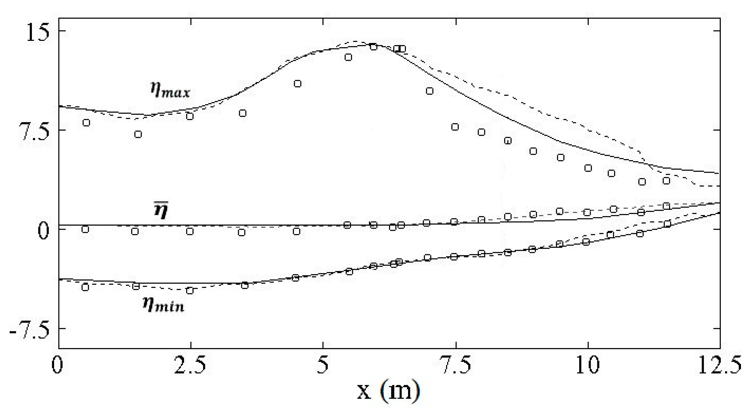
• The production of the turbulent kinetic energy dissipation is calculated by a dynamic procedure. In the surf zone the production of turbulent kinetic energy dissipation is limited by the dynamic coefficient, related to the local derivative of the free surface. Consequently, differently from the $k-\epsilon$ standard model, it is possible to limit the non-physical decrease of the wave height.

The paper is structured as follows: in Section 2 and Section 3 are presented the motion equations and modified turbulent $k-\epsilon$ model, in which vector and tensor quantities are expressed in Cartesian components on a general boundary conforming curvilinear time dependent coordinate system that includes a time-varying vertical coordinate. In Section 4 the results are shown and discussed. Conclusions are drawn in Section 5.

2. Motion Equations

We consider a transformation $x_i=x_i\left({\xi }_1,{\xi }_2,\tau \right)$, from a Cartesian coordinate system $\left(x_1,x_2,t\right)$, to a curvilinear coordinate system $\left({\xi }_1, {\xi }_2, \tau \right)$ and the inverse transformation, ${\xi }_i={\xi }_i\left(x_1,x_2,t\right)$.

In this paper we adopt a particular transformation from Cartesian to curvilinear coordinates in order to follow the free surface movements [14].

$${\xi }_1=x_1; {\xi }_2=\frac{x_2+h}{H}; \tau =t$$

(1)

in which $H\left(x_1,t\right)=h\left(x_1\right)+\eta \left(x_1,t\right)$ is the total water depth; $h$ is the undisturbed water depth and $\eta$ is the free surface elevation; ${\xi }_1$ is the horizontal boundary conforming curvilinear coordinates and ${\xi }_2$ is the time varying vertical coordinate that spans from ${\xi }_2=0$ (at the bottom) to ${\xi }_2=1$ (at the free surface). The irregular varying domain in the physical space is mapped into a regular fixed domain in the transformed space, as shown in Figure 1.

Let ${\overrightarrow{c}}_{\left(l\right)}=\partial \overrightarrow{x}/\partial {\xi }^{\left(l\right)}$ and ${\overrightarrow{c}}^{\left(l\right)}=\partial {\xi }^{\left(l\right)}/\partial \overrightarrow{x}$ $\left(l=1, 2\right)$ be the $l-th$ covariant and contravariant base vectors, respectively, and let $\overline{C}$ and $\overline{B}$ be the metric tensor and its inverse, respectively, whose components are

$$c_{lm}={\overrightarrow{c}}_{\left(l\right)}·{\overrightarrow{c}}_{\left(m\right)} c^{lm}={\overrightarrow{c}}^{\left(l\right)}·{\overrightarrow{c}}^{\left(m\right)} \left(l, m=1, 2\right)$$

(2)

The Jacobian of the transformation is given by $\sqrt{c}=\sqrt{\det \left(\overline{C}\right)}=H$.

The equations are expressed in terms of $\overline{H\overrightarrow{u}}$e $\overline{H}$, the spatial averaged values over volume elements defined in the form

$$\overline{H}=\frac{1}{\Delta L_2^{*}}{{\displaystyle \int }}_{\Delta L_2^{*}}Hd{\xi }_1$$

(3)

$$\overline{H\overrightarrow{u}}=\frac{1}{\Delta A^{*}}{{\displaystyle \int }}_{\Delta A^{*}}H\overrightarrow{u} d{\xi }_{1}d{\xi }_2$$

(4)

where $\Delta L_2^{*}=\Delta {\xi }_1$is the contour line of the control area $\Delta A^{*}=\Delta {\xi }_1\Delta {\xi }_2$ in the transformed space.

The motion equations, expressed in integral form in a time-dependent curvilinear coordinate system, are as follows:

$$\begin{gathered} \frac{\partial \overline{H\overrightarrow{u}}}{\partial \tau }=-\frac{1}{\Delta A^{*}}{\displaystyle \sum }_{\alpha =1}^2\{{{\displaystyle \int }}_{\Delta L_{\alpha }^{*}+}\left[\overrightarrow{u}\otimes \left(\overrightarrow{u}-\overrightarrow{v}\right)·\overrightarrow{c_{\left(\alpha \right)}}H\right]d{\xi }_{\beta } \\ -{{\displaystyle \int }}_{\Delta L_{\alpha }^{*}-}\left[\overrightarrow{u}\otimes \left(\overrightarrow{u}-\overrightarrow{v}\right)·\overrightarrow{c_{\left(\alpha \right)}}H\right]d{\xi }_{\beta }\}-\frac{1}{\Delta A^{*}}{\displaystyle \sum }_{\alpha =1}^2\{{{\displaystyle \int }}_{\Delta L_{\alpha }^{*}+}\left[G\eta \overrightarrow{c_{\left(\alpha \right)}}H\right]d{\xi }_{\beta } \\ -{{\displaystyle \int }}_{\Delta L_{\alpha }^{*}-}\left[G\eta \overrightarrow{c_{\left(\alpha \right)}}H\right]d{\xi }_{\beta }\}-\frac{1}{\Delta A^{*}}\frac{1}{\rho }{{\displaystyle \int }}_{\Delta A^{*}}\frac{\partial q}{\partial {\xi }^r}\overrightarrow{c_{\left(r\right)}}Hd{\xi }_{1}d{\xi }_2 \\ -\frac{1}{\Delta A^{*}}{\displaystyle \sum }_{\alpha =1}^2\{{{\displaystyle \int }}_{\Delta L_{\alpha }^{*}+}\left[2{\nu }_T\overline{S}·\overrightarrow{c_{\left(\alpha \right)}}H\right]d{\xi }_{\beta }-{{\displaystyle \int }}_{\Delta L_{\alpha }^{*}-}\left[2{\nu }_T\overline{S}·\overrightarrow{c_{\left(\alpha \right)}}H\right]d{\xi }_{\beta }\} \end{gathered}$$

(5)

where $\overrightarrow{u}$ is the fluid velocity; $\overrightarrow{v}$ is the velocity of the moving coordinate lines; $\langle \otimes \rangle$ is the outer product; $\langle ·\rangle$ is the scalar product; and $G$, $\rho ,$ and ${\nu }_T$ are, respectively, the constant of gravity, the fluid density, and the turbulent eddy viscosity. $q$ is the dynamic pressure; $2 {\nu }_T\overline{S}=\overline{R}$ is the stress tensor and $\overline{S}$ is the strain rate tensor; the $\Delta L_{\alpha }^{*}=\Delta {\xi }_{\beta }$ ($\alpha , \beta =1,2$ are cyclic) is the contour line of the area $\Delta A^{*}$ on which ${\xi }_{\alpha }$ is constant and which is located at the larger and smaller value of ${\xi }_{\alpha }$, respectively.

$$\frac{\partial \overline{H}}{\partial \tau }+\frac{1}{\Delta {\xi }_1}\left\{{{\displaystyle \int }}_{\Delta {\xi }_{2^{+}}}\left[\left(\overrightarrow{u}-\overrightarrow{v}\right)·\overrightarrow{c_{\left(\alpha \right)}}H\right]d{\xi }_2-{{\displaystyle \int }}_{\Delta {\xi }_2-}\left[\left(\overrightarrow{u}-\overrightarrow{v}\right)·\overrightarrow{c_{\left(\alpha \right)}}H\right]d{\xi }_2\right\}=0$$

(6)

where ${\xi }_2$ is the contour line of area $\Delta A^{*}$ on which ${\xi }_1$ is constant and which is located at the larger and smaller value of ${\xi }_2$, respectively.

Equations (5) and (6) are numerically solved, on a time dependent curvilinear coordinate system, where the vertical coordinate varies in time, by a finite volume shock capturing scheme, which uses an approximate HLL-type Riemann solver [15].

3. Turbulence Model

The turbulence model proposed for the simulation of the wave motion is a modified $k-\epsilon$. The governing equations are written in a boundary conforming curvilinear coordinate system in which vector and tensor quantities are expressed in Cartesian components. This form of equation does not exist in the literature.

In an original conservative form, the transport equations of turbulent kinetic energy $k$ and the dissipation rate $\epsilon$ are expressed in terms of conservative variables $\overline{Hk}$ and $\overline{H\epsilon }$ and in integral form in a curvilinear coordinate system. Let us define the following cell-averaged values in the transformed space.

$$\overline{Hk}=\frac{1}{\Delta A^{*}}{{\displaystyle \int }}_{\Delta A^{*}}kH d{\xi }_{1}d{\xi }_2$$

(7)

$$\overline{H\epsilon }=\frac{1}{\Delta A^{*}}{{\displaystyle \int }}_{\Delta A^{*}}\mathsf{\epsilon }H d{\xi }_{1}d{\xi }_2$$

(8)

The transport equation of $k$ is

$$\begin{gathered} \frac{\partial \overline{Hk}}{\partial \tau }=-\frac{1}{\Delta A^{*}}{\displaystyle \sum }_{\alpha =1}^2\{{{\displaystyle \int }}_{\Delta L_{\alpha }^{*}+}\left[k \left(\overrightarrow{u}-\overrightarrow{v}\right)·\overrightarrow{c_{\left(\alpha \right)}}\right]Hd{\xi }_{\beta }-{{\displaystyle \int }}_{\Delta L_{\alpha }^{*}-}\left[k \left(\overrightarrow{u}-\overrightarrow{v}\right)·\overrightarrow{c_{\left(\alpha \right)}}\right]Hd{\xi }_{\beta }\}+ \\ +\frac{1}{\Delta A^{*}}{\displaystyle \sum }_{\alpha =1}^2\{{{\displaystyle \int }}_{\Delta L_{\alpha }^{*}+}\left(\nu +\frac{{\nu }_T}{{\sigma }_k}\right)\frac{\partial k}{\partial {\xi }^r} \overrightarrow{c_{\left(r\right)}}· \overrightarrow{c_{\left(\alpha \right)}}Hd{\xi }_{\beta }-{{\displaystyle \int }}_{\Delta L_{\alpha }^{*}-}\left(\nu +\frac{{\nu }_T}{{\sigma }_k}\right)\frac{\partial k}{\partial {\xi }^r}\overrightarrow{c_{\left(r\right)}}· \overrightarrow{c_{\left(\alpha \right)}}Hd{\xi }_{\beta }\}+ \\ +\frac{1}{\Delta A^{*}}{{\displaystyle \int }}_{\Delta A^{*}}\left(P-\epsilon \right) H d{\xi }_{1}d{\xi }_2. \end{gathered}$$

(9)

The transport equation of $\epsilon$ is

$$\begin{gathered} \frac{\partial \overline{H\epsilon }}{\partial \tau }=-\frac{1}{\Delta A^{*}}{\displaystyle \sum }_{\alpha =1}^2\{{{\displaystyle \int }}_{\Delta L_{\alpha }^{*}+}\left[\epsilon \left(\overrightarrow{u}-\overrightarrow{v}\right)·\overrightarrow{c_{\left(\alpha \right)}}\right]Hd{\xi }_{\beta }-{{\displaystyle \int }}_{\Delta L_{\alpha }^{*}-}\left[\epsilon \left(\overrightarrow{u}-\overrightarrow{v}\right)·\overrightarrow{c_{\left(\alpha \right)}}\right]Hd{\xi }_{\beta }\}+ \\ +\frac{1}{\Delta A^{*}}{\displaystyle \sum }_{\alpha =1}^2\{{{\displaystyle \int }}_{\Delta L_{\alpha }^{*}+}\left(\nu +\frac{{\nu }_T}{{\sigma }_{\epsilon }}\right) \frac{\partial \epsilon }{\partial {\xi }^r}\overrightarrow{c_{\left(r\right)}}·\overrightarrow{c_{\left(\alpha \right)}}Hd{\xi }_{\beta }-{{\displaystyle \int }}_{\Delta L_{\alpha }^{*}-}\left(\nu +\frac{{\nu }_T}{{\sigma }_{\epsilon }}\right)\frac{\partial \epsilon }{\partial {\xi }^r}\overrightarrow{c_{\left(r\right)}}·\overrightarrow{c_{\left(\alpha \right)}}Hd{\xi }_{\beta }\}+ \\ +\frac{1}{\Delta A^{*}}{{\displaystyle \int }}_{\Delta A^{*}}\frac{\epsilon }{k}\left(C_{1\epsilon }P-C_{2\epsilon }\epsilon \right) H d{\xi }_{1}d{\xi }_2. \end{gathered}$$

(10)

The kinematic viscosity of water is $\nu$ and the turbulent eddy viscosity is calculated by

$${\nu }_T=C_{\mu }\frac{k^2}{\epsilon }.$$

(11)

In Equations (9)–(11) ${\sigma }_k$, ${\sigma }_{\epsilon }$, and $C_{\mu }$ are constant coefficients given by

$${\sigma }_k=0.72; {\sigma }_{\epsilon }=0.72;\mathrm{and}{C}_{\mu }=0.09.$$

(12)

The novelties of the $k-\epsilon$ model with respect to the standard one consist of the following:

• The coefficient $C_{2\epsilon }$ is determined by a dynamic procedure proposed by Yakhot et al. [20]:

  $$C_{2\epsilon }=1.68+\frac{C_{\mu }{\zeta }^3\left(1-\zeta /4.38\right)}{1+0.012{\zeta }^3}$$

  (13)

  where $\zeta =\frac{k}{\epsilon }\sqrt{2\overline{S}\overline{S}}$.
• The closure relation that limits the production of dissipation rate is proposed as a function of the local derivative of the free surface.

  $$C_{1\epsilon }=2.15-\left(2.15-1.42\right)B\left(x\right)$$

  (14)

  $C_{1\epsilon }$ varies between $\left(1.42÷2.15\right)$; $B\left(x\right)$ is a linear function and it is related to the steepness of the wave front $\left(\partial \eta /\partial t\right)$:

  $$B\left(x\right)=\{\begin{array}{c}0 se \partial \eta /\partial t\le 0.15\sqrt{g{h}_0}\\ 0-1 se 0.15\sqrt{g{h}_0}<\partial \eta /\partial t\le 0.3\sqrt{g{h}_0}\\ 1 se \partial \eta /\partial t>0.3\sqrt{g{h}_0}\end{array}$$

  (15)
• The closure relation of the production of turbulent kinetic energy takes into account the nonlinear terms and is given by

  $$P={{\displaystyle \int }}_{\Delta A^{*}}-\overline{R}:\frac{\partial \overrightarrow{u}}{\partial {\xi }_{\alpha }}\otimes \overrightarrow{c_{\left(\alpha \right)}}Hd{\xi }_{1}d{\xi }_2$$

  (16)

  where $\langle :\rangle$ is the scalar inner product between the second order tensors.
  The Reynolds stress $\overline{R}$ is calculated by a nonlinear model and is expressed in a boundary conforming curvilinear grid, in which vector and tensor quantities are given in terms of Cartesian components:

  $$\begin{gathered} \overline{R}=-C_d\frac{k^2}{\epsilon }\left[\frac{\partial \overrightarrow{u}}{\partial {\xi }_{\alpha }}\otimes \overrightarrow{c_{\left(\alpha \right)}}+{\left(\frac{\partial \overrightarrow{u}}{\partial {\xi }_{\alpha }}\otimes \overrightarrow{c_{\left(\alpha \right)}}\right)}^T\right]+k\overline{I}-C_1\frac{k^3}{{\epsilon }^2}\{[\left(\frac{\partial \overrightarrow{u}}{\partial {\xi }_{\alpha }}\otimes \overrightarrow{c_{\left(\alpha \right)}}·\frac{\partial \overrightarrow{u}}{\partial {\xi }_{\alpha }}\otimes \overrightarrow{c_{\left(\alpha \right)}}\right) \\ +{\left(\frac{\partial \overrightarrow{u}}{\partial {\xi }_{\alpha }}\otimes \overrightarrow{c_{\left(\alpha \right)}}·\frac{\partial \overrightarrow{u}}{\partial {\xi }_{\alpha }}\otimes \overrightarrow{c_{\left(\alpha \right)}}\right)}^T]-\left(\frac{\partial \overrightarrow{u}}{\partial {\xi }_{\alpha }}\otimes \overrightarrow{c_{\left(\alpha \right)}}·\frac{\partial \overrightarrow{u}}{\partial {\xi }_{\alpha }}\otimes \overrightarrow{c_{\left(\alpha \right)}}\right)\overline{I}\} \\ -C_2\frac{k^3}{{\epsilon }^2}\{\left[\frac{\partial \overrightarrow{u}}{\partial {\xi }_{\alpha }}\otimes \overrightarrow{c_{\left(\alpha \right)}}·{\left(\frac{\partial \overrightarrow{u}}{\partial {\xi }_{\alpha }}\otimes \overrightarrow{c_{\left(\alpha \right)}}\right)}^T\right]-\frac{1}{2} \left[\frac{\partial \overrightarrow{u}}{\partial {\xi }_{\alpha }}\otimes \overrightarrow{c_{\left(\alpha \right)}}·{\left(\frac{\partial \overrightarrow{u}}{\partial {\xi }_{\alpha }}\otimes \overrightarrow{c_{\left(\alpha \right)}}\right)}^T\right]\overline{I}\} \\ -C_3\frac{k^3}{{\epsilon }^2}\{\left[{\left(\frac{\partial \overrightarrow{u}}{\partial {\xi }_{\alpha }}\otimes \overrightarrow{c_{\left(\alpha \right)}}\right)}^T·\frac{\partial \overrightarrow{u}}{\partial {\xi }_{\alpha }}\otimes \overrightarrow{c_{\left(\alpha \right)}}\right]-\frac{1}{2}\left[{\left(\frac{\partial \overrightarrow{u}}{\partial {\xi }_{\alpha }}\otimes \overrightarrow{c_{\left(\alpha \right)}}\right)}^T·\frac{\partial \overrightarrow{u}}{\partial {\xi }_{\alpha }}\otimes \overrightarrow{c_{\left(\alpha \right)}}\right]\overline{I}\} \end{gathered}$$

  (17)

  where $T$ expresses the transposed terms; $\overline{I}$ is the identity tensor; $C_d$, $C_1$, $C_2$, and $C_3$ are empirical coefficients:

  $$\begin{gathered} C_d=\frac{2}{3}\left(\frac{1}{7.4+2S_{max}}\right)\hspace{1em}\hspace{1em}{C}_1=\frac{1}{185.2+3D_{max}} \\ {C}_2=-\frac{1}{58.8+2D_{max}^2}\hspace{1em}\hspace{1em}{C}_3=\frac{1}{370.4+3D_{max}^2} \end{gathered}$$

  (18)

  where

  $$S_{max}=\frac{k}{\epsilon }max\left\{\left|\frac{\partial u_i}{\partial x_i}\right|\right\}\hspace{1em}\hspace{1em}{D}_{max}=\frac{k}{\epsilon }max\left\{\left|\frac{\partial u_i}{\partial x_j}\right|\right\}.$$

  (19)
  The boundary conditions on the bottom concern the turbulent kinetic energy and the dissipation rate:

  $$k=\frac{{u^{*}}^2}{\sqrt{C_{\mu }}} \hspace{1em}\hspace{1em}\epsilon =\frac{{u^{*}}^3}{Ky}$$

  (20)

  where $u^{*}$ represents the friction velocity:

  $$\frac{u^{*}}{u}=\frac{1}{K}\ln \left(\frac{u^{*}}{k_s/30}\right).$$

  (21)

  $K=0.4$ is the von Karman constant and $k_s=0.0002$ is the roughness.

4. Results

In this section the numerical results obtained by the Gallerano et al. [14] numerical model are compared with the experimental measurements by Ting and Kirby [21]. The test conducted by Ting and Kirby [21] consisted of realizing a spilling breaking wave on a sloping beach. It is possible to examine the wave energy dissipation in the surf zone due to the turbulence by means of the turbulence model. The experimental wave tank was $40\mathrm{m}$ long, $0.6\mathrm{m}$ wide, and $1.0\mathrm{m}$ deep and consisted of a beach with a constant slope equal to $1:35$ connected to a region with a constant depth equal to $h=0.4\mathrm{m};$ the wavemaker was placed at the left end of the wave tank. In this paper, in order to save computational time, we numerically reproduced only the final eighteen meters of the experimental arrangement shown in Figure 2, and the abscissa $x=0 \mathrm{m}$ indicates the toe of the slope where the still water depth is equal to $h=0.38 \mathrm{m}$.

The computational grid adopted for all the numerical simulations consisted of $\mathrm{13,728}$ grid cells in the horizontal direction in which $x_1$ spanned from $-1 \mathrm{m}$ to $-17 \mathrm{m}$ and the grid spacing was $\Delta x_1=0.025 \mathrm{m}$. In the vertical direction, $13$ grid cells were used. As shown in Figure 3, the mesh was refined at the top and bottom boundaries. For this test, cnoidal waves with period $T=2 \mathrm{s}$ and wave height $H=0.125\mathrm{m}$ were imposed as input boundary conditions. In the swash region, a wetting–drying treatment was used.

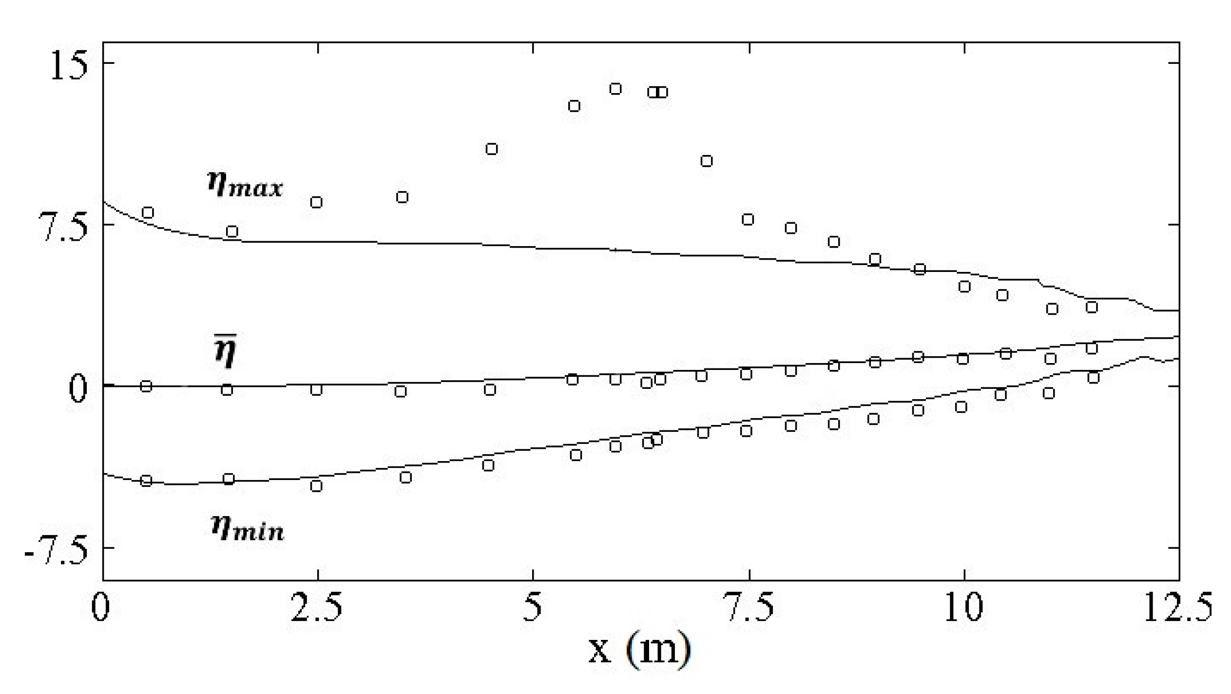
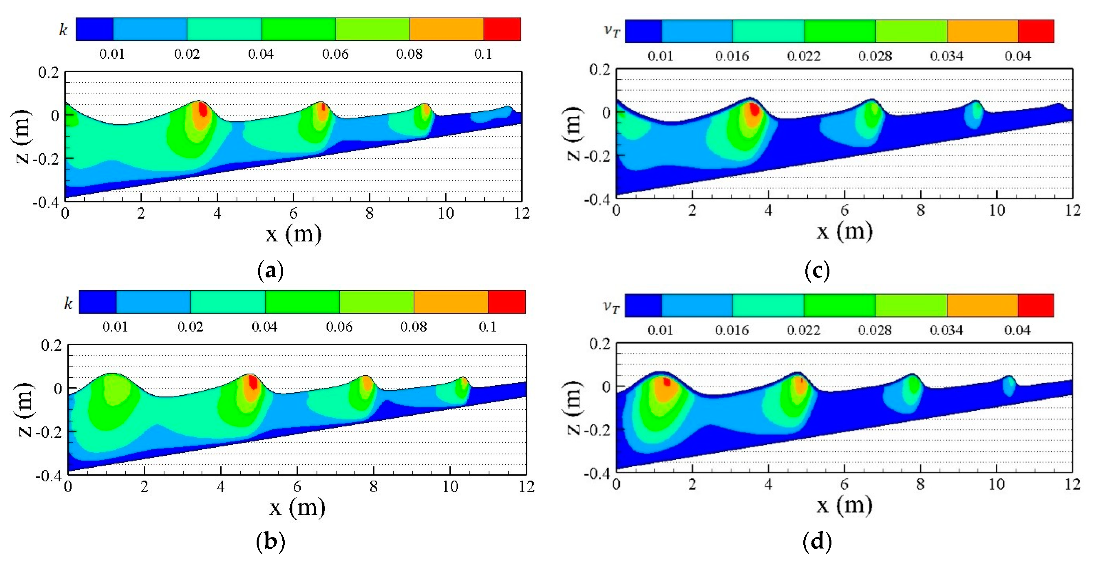
4.1. Spilling Breaking Test without Turbulence Model

In this subsection we present briefly the numerical results obtained without the turbulence model [22].

Figure 4 shows the distribution of the wave crest and wave trough in the cross-shore direction, together with the mean water level, obtained by the Gallerano et al. [14] numerical model in which the turbulence model was switched off. The mean water level and the wave crest and trough, shown in Figure 4, were computed by performing, respectively, a time-average and a phase-average, over five wave periods of the date extracted from the numerical simulation, once the simulation reached a quasi-stationary state. In the same figure, the experimental results by Ting and Kirby [21] and the numerical results by Ma [12] are also shown. In the shoaling zone ($x<6.4 \mathrm{m}$) the numerical results obtained by the Gallerano et al. [14] numerical model fit quite well with the experimental results, while after the initial wave breaking point ($x>6.4 \mathrm{m}$) the numerical results overestimated the experimental ones. As shown in Figure 4, similar numerical results were obtained by Ma et al. [12].

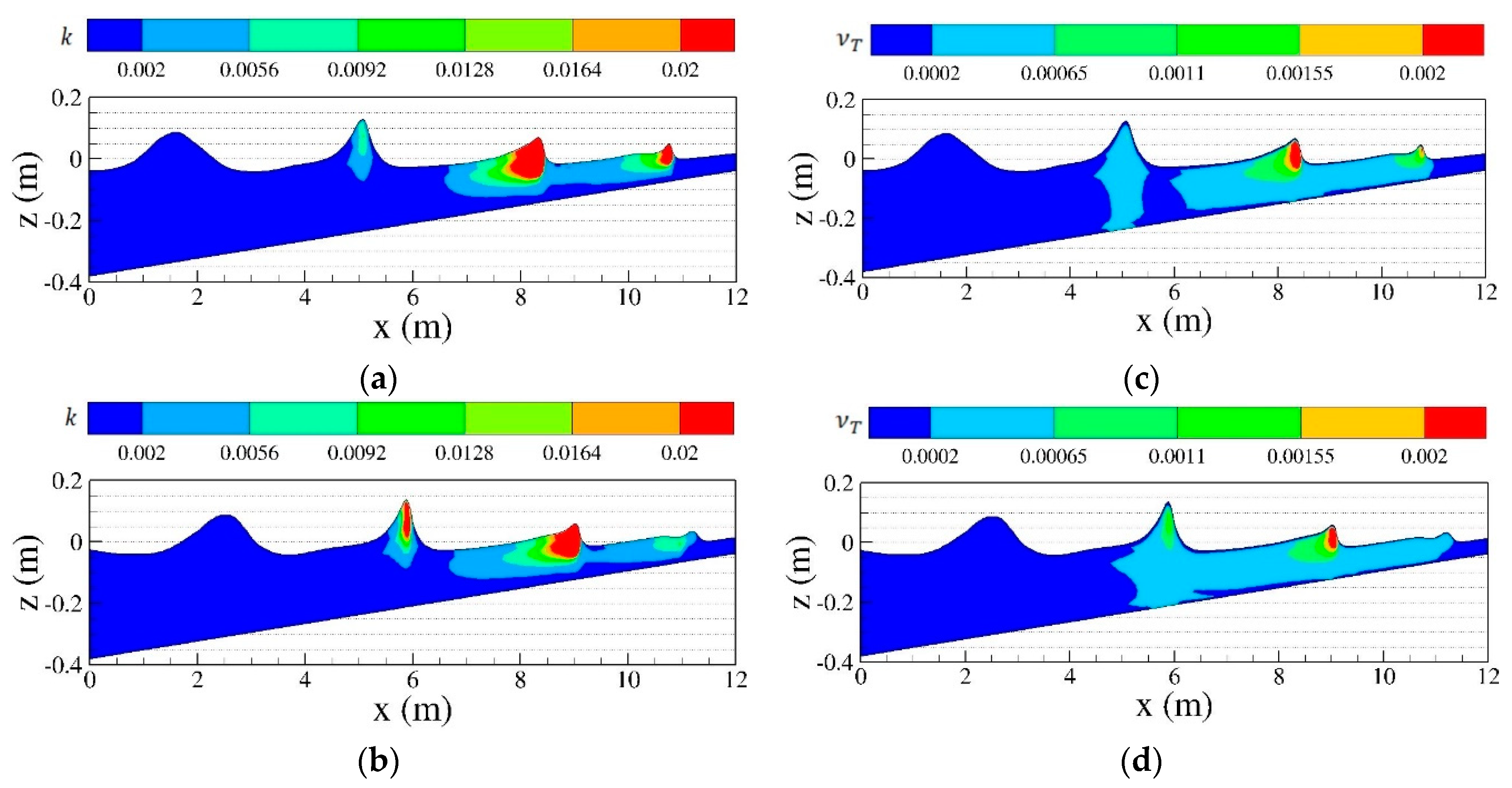
4.2. Spilling Breaking Test with Turbulence Model

Figure 5 shows the distribution of the wave crest and wave trough in the cross-shore direction, together with the mean water level, obtained by the Gallerano et al. [14] numerical model in which the turbulence model is the standard $k-\epsilon$ proposed by Rodi [23]. From this figure, it is possible to notice that for this test case the standard $k-\epsilon$ turbulence model produces an excessive non-physical decrease in the wave height with respect to the experimental results [21].

Figure 6 shows a snapshot of the instantaneous spatial distribution of the turbulent kinetic energy (a,b) and the turbulent eddy viscosity (c,d), in two different time steps, obtained by the Gallerano et al. [14] numerical model in which the turbulence model is the standard$k-\epsilon$ proposed by Rodi [23]. From this figure, it can be noticed that the turbulent kinetic energy is generated in correspondence with the wave fronts in all the surf zone, also before $x=6.4 \mathrm{m}$, where the initial wave breaking point is located according to the experimental measurements [21]. Figure 6 also shows that, by using the standard $k-\epsilon$ turbulence model [23], the simulated wave fronts are very smooth, due to an excess of the turbulent eddy viscosity produced by the modelled turbulent kinetic energy.

From Figure 5 and Figure 6 it can be deduced that, for this test case, the standard $k-\epsilon$ turbulence model [23] produces an excess of turbulent kinetic energy and turbulent eddy viscosity, which entails very small simulated wave heights and very smooth wave fronts in the whole surf zone.

Figure 7 shows the distribution of the wave crest and wave trough in the cross-shore direction, together with the mean water level, obtained by the Gallerano et al. [14] numerical model in which the turbulence model is the modified $k-\epsilon$ turbulence proposed in this paper. In the same figure, the above numerical results are compared with the experimental results by Ting and Kirby [21] and the numerical results obtained by the Gallerano et al. [14] numerical model in which the turbulence model is switched off. From this figure, it is possible to notice that the initial wave breaking point is correctly predicted by the modified $k-\epsilon$ turbulence model; the modified $k-\epsilon$ turbulence model adequately represents the distribution of the wave crest and wave trough before and after the initial wave breaking point.

Figure 8 shows a snapshot of the instantaneous spatial distribution of the turbulent kinetic energy (a,b) and the turbulent eddy viscosity (c,d), in two different time steps, obtained by the Gallerano et al. [14] numerical model in which the turbulence model is the proposed modified $k-\epsilon$. From this figure, it can be noticed that the turbulent kinetic energy is generated, in correspondence with the wave fronts, mainly after the initial wave breaking point ($x>6.4 \mathrm{m}$), where the wave turbulence processes are significant.

The comparison between Figure 6 and Figure 8 shows that, under breaking waves, the modified $k-\epsilon$ turbulence model produces lower values of turbulent kinetic energy with respect to the standard one.

Figure 9 shows the vertical time-mean cross-shore horizontal velocity component and the turbulent kinetic energy obtained by the proposed modified $k-\epsilon$ turbulence model (crosses), in comparison with the experimental results (empty circles) by Ting and Kirby [21] at $x=7.25\mathrm{m}$. From this figure, it is possible to notice a good agreement between the numerical and the experimental results for both the quantities.

5. Conclusions

A modified $k-\epsilon$ turbulence model was proposed that is able to simulate the hydrodynamic field and the turbulent kinetic energy under a breaking wave.

In order to numerically simulate the wave propagation from deep water to the shoreline and the wave breaking, a numerical model was used in which the vector and tensor quantities are expressed in Cartesian components, where only the vertical coordinate is expressed as a function of a time-dependent curvilinear coordinate that follows the free surface movements.

It was demonstrated that the shock-capturing model, defined in the context of $\sigma$-coordinate, underestimates the energy dissipation at the breaking point and consequently overestimates the wave height in the surf zone.

In this paper, a modified $k-\epsilon$ turbulence model was proposed based on a dynamic procedure in order to contain the production of kinetic energy dissipation in the surf zone and limit the destruction of the turbulent kinetic energy dissipation. It was demonstrated that the proposed turbulence model is capable of correctly estimating the energy dissipation induced by the wave breaking, in order to avoid any underestimation of the wave height.

References

- Cannata, G.; Barsi, L.; Petrelli, C.; Gallerano, F. Numerical investigation of wave fields and currents in a coastal engineering case study. WSEAS Trans. Fluid Mech. 2018, 13, 87–94. [Google Scholar]
- Shi, F.; Kirby, J.T.; Harris, J.C.; Geiman, J.D.; Grilli, S.T. A high-order adaptive time-stepping TVD solver for Boussinesq modelling of breaking waves and coastal inundation. Ocean Model. 2012, 43–44, 36–51. [Google Scholar] [CrossRef]
- Gallerano, F.; Cannata, G.; De Gaudenzi, O.; Scarpone, S. Modeling bed evolution using weakly coupled phase-resolving wave model and wave-averaged sediment transport model. Coast. Eng. J. 2016, 58. [Google Scholar] [CrossRef]
- Cannata, G.; Petrelli, C.; Barsi, L.; Fratello, F.; Gallerano, F. A dam-break flood simulation model in curvilinear coordinates. WSEAS Trans. Fluid Mech. 2018, 13, 60–70. [Google Scholar]
- Kazolea, M.; Ricchiuto, M. On wave breaking for Boussinesq-type models. Ocean Model. 2018, 123, 16–39. [Google Scholar] [CrossRef]
- Fredsøe, J.; Andersen, O.H.; Silberg, S. Distribution of Suspended Sediment in Large Waves. J. Waterw. Port Coast. Ocean Eng. 1985, 111, 1041–1059. [Google Scholar] [CrossRef]
- Deigaard, R.; Fredsøe, J.; Hedegaard, I.B. Suspended sediment in the surf zone. J. Waterw. Port Coast. Ocean Eng. 1986, 112, 115–128. [Google Scholar] [CrossRef]
- Rakha, K.A. A Quasi-3D phase-resolving hydrodynamic and sediment transport model. Coast. Eng. 1998, 34, 277–311. [Google Scholar] [CrossRef]
- Harlow, F.H.; Welch, J.E. Numerical Calculation of Time-Dependent Viscous Incompressible Flow of Fluid with Free Surface. Phys. Fluids 1965, 8, 2182–2189. [Google Scholar] [CrossRef]
- Bradford, S.F. Numerical Simulation of Surf Zone Dynamics. J. Waterw. Port Coast. Ocean Eng. 2000, 126, 1–13. [Google Scholar] [CrossRef]
- Phillips, N.A. A coordinate system having some special advantages for numerical forecasting. J. Meteorol. 1956, 14, 184–185. [Google Scholar] [CrossRef]
- Ma, G.; Shi, F.; Kirby, J.T. Shock-capturing non-hydrostatic model for fully dispersive surface wave processes. Ocean Model. 2012, 43–44, 22–35. [Google Scholar] [CrossRef]
- Cannata, G.; Petrelli, C.; Barsi, L.; Camilli, F.; Gallerano, F. 3D free surface flow simulations based on the integral form of the equations of motion. WSEAS Trans. Fluid Mech. 2017, 12, 166–175. [Google Scholar]
- Gallerano, F.; Cannata, G.; Lasaponara, F.; Petrelli, C. A new three-dimensional finite-volume non-hydrostatic shock-capturing model for free surface flow. J. Hydrodyn. 2017, 29, 552–566. [Google Scholar] [CrossRef]
- Toro, E. Riemann Solvers and Numerical Methods for Fluid Dynamics: A practical Introduction, 3rd ed.; Springer: Berlin/Heidelberg, Germany, 2009. [Google Scholar]
- Ma, G.; Chou, Y.-J.; Shi, F. A wave-resolving model for nearshore suspended sediment transport. Ocean Model. 2014, 77, 33–49. [Google Scholar] [CrossRef]
- Bosch, G.; Rodi, W. Simulation of vortex shedding past a square cylinder with different turbulence models. Int. J. Numer. Met. Fluids 1998, 28, 601–616. [Google Scholar] [CrossRef]
- Ting, F.C.K.; Kirby, J.T. Observation of undertow and turbulence in a wave period. Costal Eng. 1994, 24, 51–80. [Google Scholar] [CrossRef]
- Lin, P.; Liu, P.L.-F. A numerical study of breaking waves in the surf zone. J. Fluid Mech. 1998, 359, 239–264. [Google Scholar] [CrossRef]
- Derakhti, M.; Kirby, J.T.; Ma, G. NHWAVE: Consistent boundary conditions and turbulence modeling. Ocean Model. 2016, 106, 121–130. [Google Scholar] [CrossRef]
- Yakhot, V.; Orszag, S.; Thangam, S.; Gatski, T.; Speziale, C. Development of turbulence models for shear flows by double expansion technique. Phys. Fluids A Fluid Dyn. 1992, 4, 1–26. [Google Scholar] [CrossRef]
- Gallerano, F.; Cannata, G.; Barsi, L.; Palleschi, F.; Iele, B. Simulation of wave motion and wave breaking induced energy dissipation. WSEAS Trans. Fluid Mech. 2019, 14, 62–69. [Google Scholar]
- Rodi, W. Examples of calculation methods for flow and mixing in stratified flows. J. Geophys. Res. 1987, 92, 5305–5328. [Google Scholar] [CrossRef]
© 2019 by the authors. Licensee MDPI, Basel, Switzerland. This article is an open access article distributed under the terms and conditions of the Creative Commons Attribution (CC BY) license (http://creativecommons.org/licenses/by/4.0/).
Share and Cite
Cannata, G.; Palleschi, F.; Iele, B.; Gallerano, F. A Modified k – ε Turbulence Model for a Wave Breaking Simulation. Water 2019, 11, 2282. https://doi.org/10.3390/w11112282
Cannata G, Palleschi F, Iele B, Gallerano F. A Modified k – ε Turbulence Model for a Wave Breaking Simulation. Water. 2019; 11(11):2282. https://doi.org/10.3390/w11112282
Chicago/Turabian StyleCannata, Giovanni, Federica Palleschi, Benedetta Iele, and Francesco Gallerano. 2019. "A Modified k – ε Turbulence Model for a Wave Breaking Simulation" Water 11, no. 11: 2282. https://doi.org/10.3390/w11112282
APA StyleCannata, G., Palleschi, F., Iele, B., & Gallerano, F. (2019). A Modified k – ε Turbulence Model for a Wave Breaking Simulation. Water, 11(11), 2282. https://doi.org/10.3390/w11112282