In this paper, the methodology is based on a GIS-based spatial assessment process for flood hazard and conducted by using multi-criteria analysis concepts and an AHP, WR and RW frameworks. This approach used the spatial data management capabilities of GIS and the flexibility of MCDA to combine factual evidence with value-based information. MCDA is a systematic procedure for designing, evaluating and selecting decision alternatives on the basis of conflicting criteria. The motivation of integrating GIS and MCDA stems from the need to make the geographic information technology more relevant for analyzing decisions. Spatial or GIS-based MCDA can be thought of as a collection method for transforming and combining geographic data and preferences (value judgments) to obtain information for decision-making. The factual evidences considered in this paper were slope, elevation, soil type, rainfall, drainage density and distance to the main channel, and defined as indicators. The value-based information approach, following Saaty [
34], uses an expert decision to identify which indicators are the most crucial in flood hazard map.
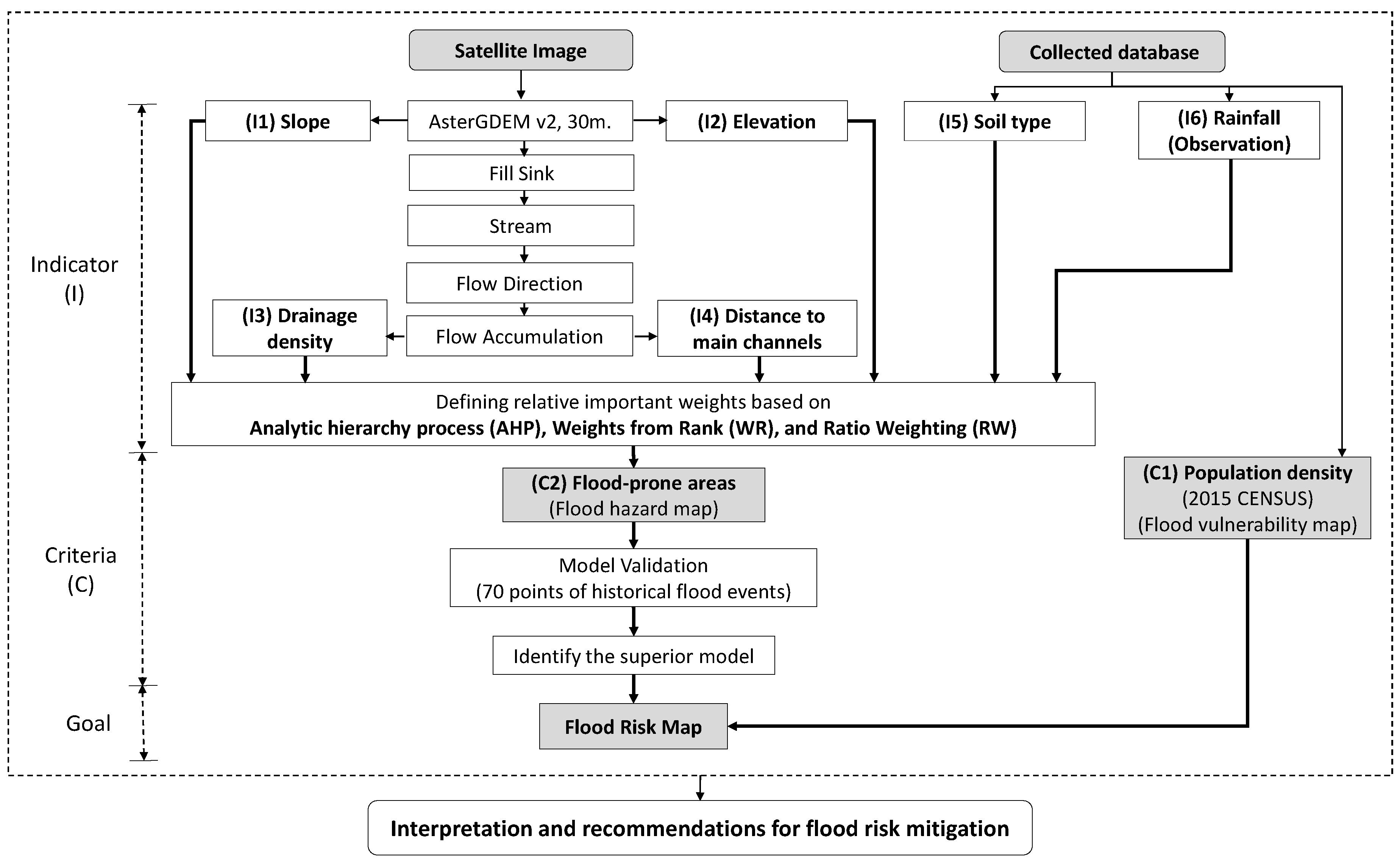
Figure 3 presents the flowchart of the methodology applied in this paper.
4.1. Indicators and Criteria
An important step of this analysis is the criteria selection for evaluating the flood risk map. The criteria considered are two, flood hazard and vulnerability. The barangay population density was used as the indicator in the vulnerability assessment. There are many indicators affecting flood hazard identification and modeling, and they vary from one study area to another. For instance, urban flood modeling is incredibly complex compared to rural flood modeling due to the interactions with manmade structures such as buildings, roads, channels, tunnels and underground structures. This paper used a composite flood hazard map index based on following six indicators. These indicators were selected based on various case studies [
1,
2,
15,
16,
33] and based on the available data in the study area.
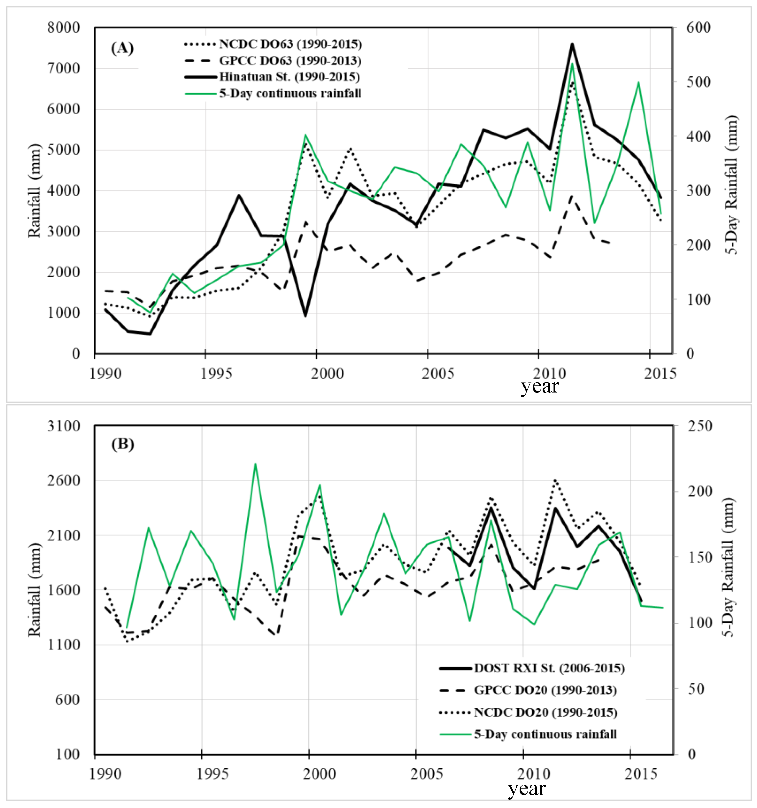
(1) Rainfall: At any location, the chance of flooding increases as the amount of rain increases. Higher rainfall intensity can result in more runoff because the ground cannot quickly absorb the water. In this study, the 5-day continuous maximum rainfall in every year was determined for 1991–2016 as shown in
Figure 2. Then, the average of the 5-day continuous maximum rainfall over the 25 years was used in the analysis. Due to the limited number of weather stations in the study area, data from the NCDC was used in this study (
Table S1). A spatial interpolation was performed to obtain the data for the study area by using the Kriging interpolation method, as in other case studies [
5,
50,
51,
52]. The spatial distribution of the 5-day continuous rainfall is illustrated in
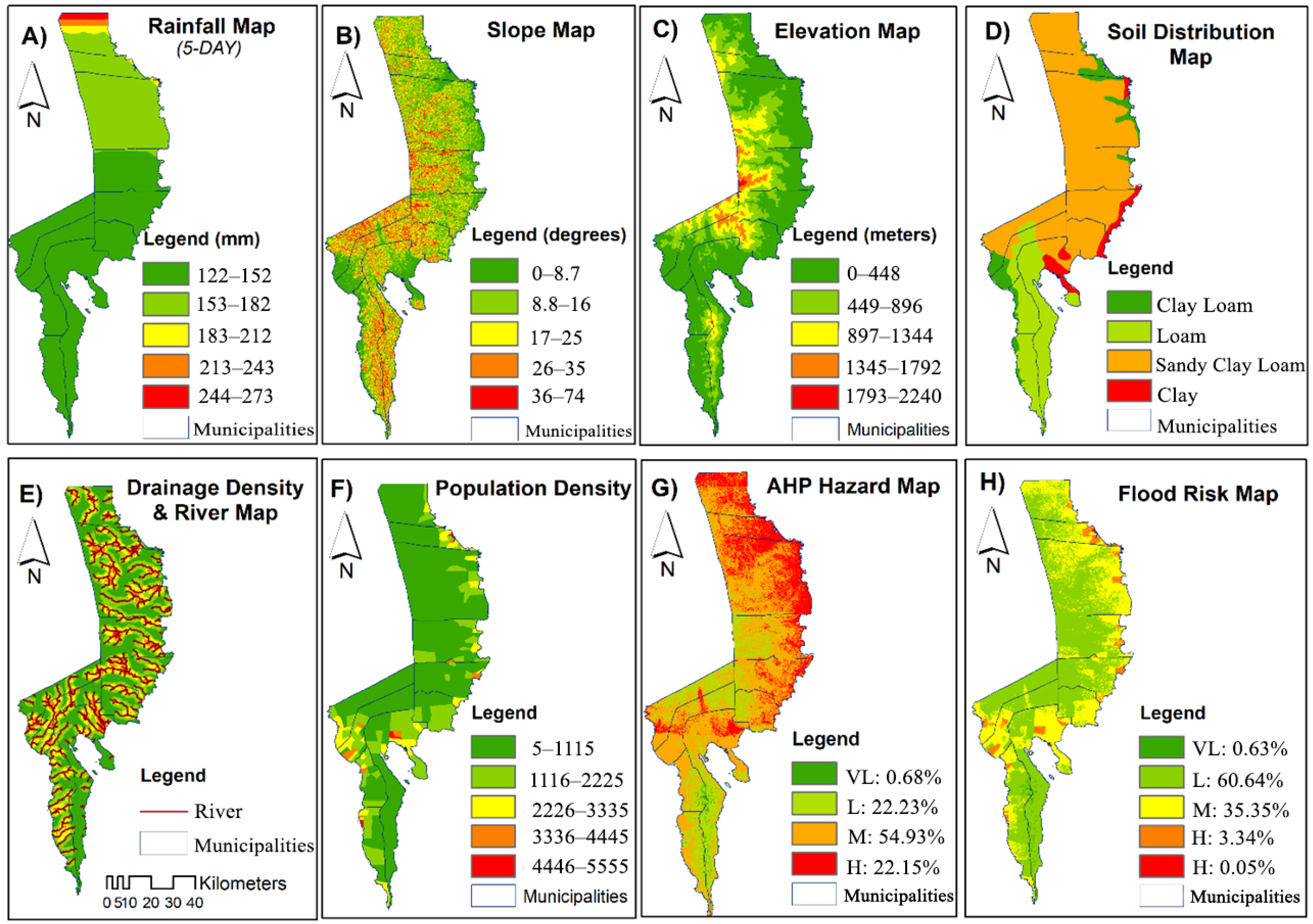
Figure 4A.
(2) Slope: The slope is one of the crucial elements in flooding. The danger of flooding increases as the slope decrease. The slope is a reliable indicator of flood susceptibility [
53]. The slope is presented in
Figure 4B.
(3) Elevation: In contrast, the elevation of an area is a major factor in flooding. Low elevation is a good indicator of areas with a high potential for flood accumulation. Water flows from higher to lower elevations; therefore, slope influences the amount of surface runoff and infiltration [
5]. Flat areas at low elevations may flood more quickly than areas at higher elevations with steeper slopes [
5]. The elevation is appeared in
Figure 4C.
(4) Soil: Soil type is a significant factor in determining the water holding and infiltration characteristics of an area and consequently affects flood susceptibility [
54,
55]. Generally, runoff from intense rainfall is likely to be faster and greater in clay soils than in sand [
56]. Additionally, rain runoff from intense rainfall is likely to be faster and greater in loam than in sand. The soil type of Davao Oriental is shown in
Figure 4D.
(5) Drainage density: Drainage density is the length of all channels within the basin divided by the area of the basin [
2]. A dense drainage network is a good indicator of flow accumulation pathways and of areas with a high potential for flooding [
53]. The drainage density and distance to the main channel are exhibited in
Figure 4E.
(6) Distance to the main channel: Distance to the main channel significantly impacts flood mapping. Areas located close to the main channel and flow accumulation path are more likely to flood [
4,
53].
Once the six indicators were defined, the next step was to build the spatial database. Each indicator was converted into raster data with a 30 m × 30 m grid resolution. The ASTER GDEM data were registered and projected to the UTM coordinate system zone 51N. The slope and elevation were obtained using the 3D Analyst algorithm based on a DEM. The drainage density and distance to the main channel were obtained using Arc Hydro, which is a set of data models that operate within ArcGIS to support geospatial and temporal data analyses. All data were integrated into the GIS environment using the AHP, WR and RW methods. Finally, the weighted overlay was used to calculate the flood hazard, which was then combined with the flood vulnerability to assess a flood risk in the study area.
4.2. Analytic Hierarchy Process
The AHP is a systematic approach developed in the 1970s to give decision-making based on experience, intuition and heuristics derived from sound mathematical principles [
57]. It helps structure the decision-maker’s thoughts and can help in organizing the problem in a way that is simple to follow and analyze. Basically, the AHP helps in structuring the complexity, measurement and synthesis of rankings [
58]. Therefore, these features make it suitable for a wide variety of applications, including alternative selection, resource allocation, forecasting, business process re-engineering, quality function development, benchmarking, public policy decisions, healthcare, hazard mapping, risk analysis and many more [
57].
The AHP provides a means of decomposing the problem into a hierarchy of sub-problems, which can be more easily comprehended and subjectively evaluated. The subjective evaluations are converted into numerical values and processed to rank each alternative (indicator in this study) on a numerical scale. It can be explained in the following steps:
Step 1: The problem is decomposed into a hierarchy of goal, criteria and indicators. Structuring the decision problem as a hierarchy is fundamental and the most important part in the process of the AHP. The hierarchy illustrates a relationship between elements of one level with those of the level immediately below.
Figure 3 shows a tree structure representing an inverted hierarchy structure. At the root of the inverted hierarchy is the goal (to produce a flood risk map) of the problem being studied and analyzed. The leaf nodes are the six indicators to be compared.
Step 2: Data are collected from experts or decision-makers corresponding to the hierarchy structure, in the pairwise comparison of indicators based on a qualitative scale between 1 (equally important) and 9 (extremely important) proposed by Saaty [
34] (see,
Table S2 for the Saaty scale in the Supplementary Material). For each pairing within each criterion, a higher number means that the chose indicator is considered more important than the other indicator used in the comparison. Four local experts from the province of Davao Oriental in the field of natural disaster provided their judgments of the relative importance of one indicator against another (
Table S3).
Step 3: The pairwise comparison of the six indicators generated at step 2 above are organized into a square matrix, the pairwise comparison matrix (
Table 2). The diagonal elements of the matrix are 1. The indicator in the
ith row is more important that the indicator in
jth column if the value of element (
i,
j) is larger than 1; otherwise the indicator in the
jth column is more important than in the
ith row. The (
j,
i) element of the matrix is the reciprocal of the (
i,
j) element.
Step 4: The pairwise comparison matrix from step 3 is then normalized by Equation (1). Then, the priority vector (PV) is derived by dividing the sum of the normalized column of the matrix by the number of indicators, n, as shown in Equation (2).
where C
ij is the value of an indicator in the pairwise comparison matrix, X
ij is the normalized score and PV
ij is the priority vector. The PVs give the relative importance of the indicators being compared and represent the weights of the indicators.
Table 3 depicts the normalized comparison matrix and the PVs.
Step 5: The consistency of the normalized comparison matrix is evaluated as described below. Since the numeric values of the matrix are derived from the subjective judgments of experts, it is impossible to avoid some inconsistency in the final matrix of their judgments [
59]. Then, the question is how much inconsistency is acceptable. For this purpose, the AHP calculates a consistency ratio (CR) comparing the consistency index (CI) of the final normalized comparison matrix with that of a random-like matrix (RI). Saaty [
34] provides the calculated RI value for matrices of different sizes (
Table S4).
Firstly, use the PV as weights of each column of the pairwise comparison matrix as shown in
Table S5. Secondly, multiply each value in the first column of the pairwise comparison matrix in
Table S5 by the PV of first indicator as shown in the first column of
Table S6; continue this process for all the columns.
Table S6 shows the resulting matrix. Thirdly, add the values in each row to obtain the weighted sum as shown in
Table S7. Fourthly, divide the weighted sums by the corresponding PVs of each indicator to obtain the consistency measure (CM) as shown in
Table S8. Fifthly, calculate the average of CMs,
. Lastly, calculate the CI and CR by the followings.
The λ
max was 6.121 obtained from
Table S8 and then the CI was 0.024 with n = 6. Therefore, by dividing the CI by RI (1.24 for
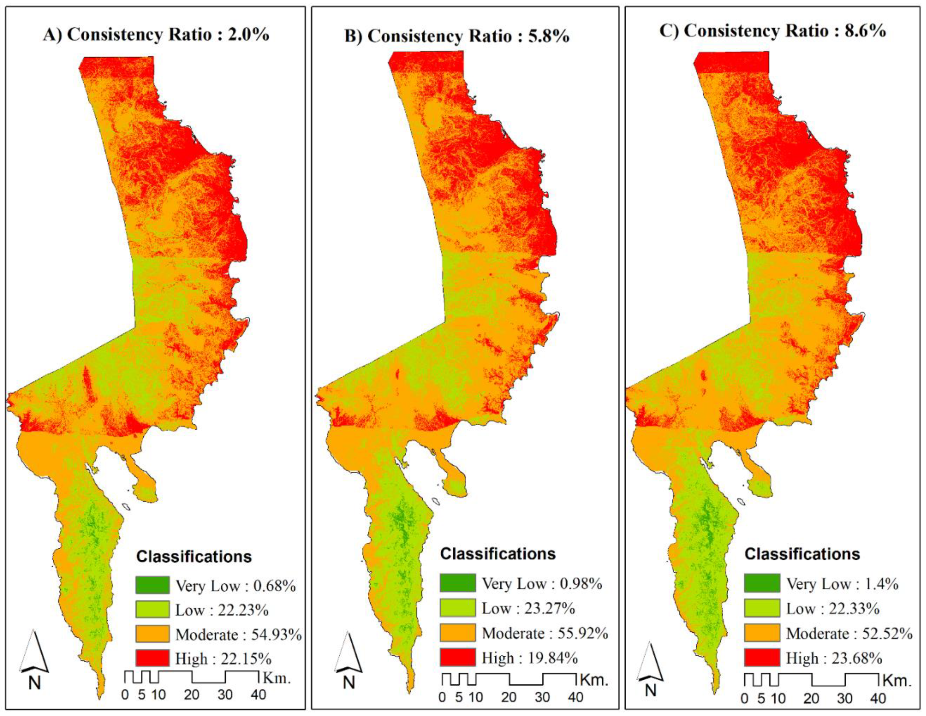
n = 6 from Saaty), the CR was obtained as 0.02. Saaty suggests the value of CR should be less than 1 to have an acceptable consistency. Since the CR was 0.02 in this case, it can be assumed that the comparison matrix was reasonably consistent so that we could continue the decision-making process using AHP.
Step 6: By multiplying the six indicators by the corresponding weights and aggregating them, the hazard index (HI) is obtained by:
where St, Sl, Dd, Dc, E and R represent the six indicators, soil type, slope, drainage, distance to main channel, elevation and rainfall, respectively.
4.3. Weights by Rank
In this method, the weight of indicator is arranging through a rank order. In that way, every indicator is ranked as per decision-maker preference. The decision-makers were the same four local experts considered in the AHP analysis. The most important is 1, the next is 2 and so on. The ranking of the indicators from the experts are shown in
Table S9. Once ranking is established for a set of indicators, the numerical weights are calculated using Equation (6).
where W
i is the normalized weight for
ith indicator, n is the total number of indicators under consideration (j = 1, 2, …, n) and r
j is the rank position of
jth indicator. Each indicator is weighted (n − r
i + 1) and then normalized by the sum of all weights ∑(n − r
j + 1). Therefore, the ranking method estimated weight should be considered as an approximation [
60]. The results are given in
Table 4. The average rank (AR) values are the average results from the four experts in the study area. Then, the resulting weight (W) in
Table 4 was used to calculate the HI as shown in Equation (7).
4.4. Ratio Weighting
In this method, it also uses the pairwise comparisons to establish the relative importance among indicators. It is also likely that the pairwise comparisons will be inconsistent. Therefore, this approach requires more information to compensate for the inconsistencies of judgments. Efficient techniques to retrieve weights from pairwise comparison data include the simplified prioritization method as follows [
61]:
Step 1: A decision-maker assesses importance (weight) ratios between indicators using pairwise comparisons. In this study, the same local experts in Davao Oriental ranked the indicators.
Table S10 shows the comparison matrix based on the expert’s judgments among the indicators.
Step 2: Compute the geometric mean of each row of the comparison matrix in
Table S10, and then normalize the resulting numbers. The geometric mean and the numerical weights are calculated using Equations (8) and (9).
Table 4 depicts the resulting geometric mean and weights of the judgments.
where GM
i is the geometric mean for
ith indicator, n is the total number of indicators and W
i is the normalized weight for
ith indicator. The HI is computed by using the average weight (AW) in
Table 4 as in Equation (10).
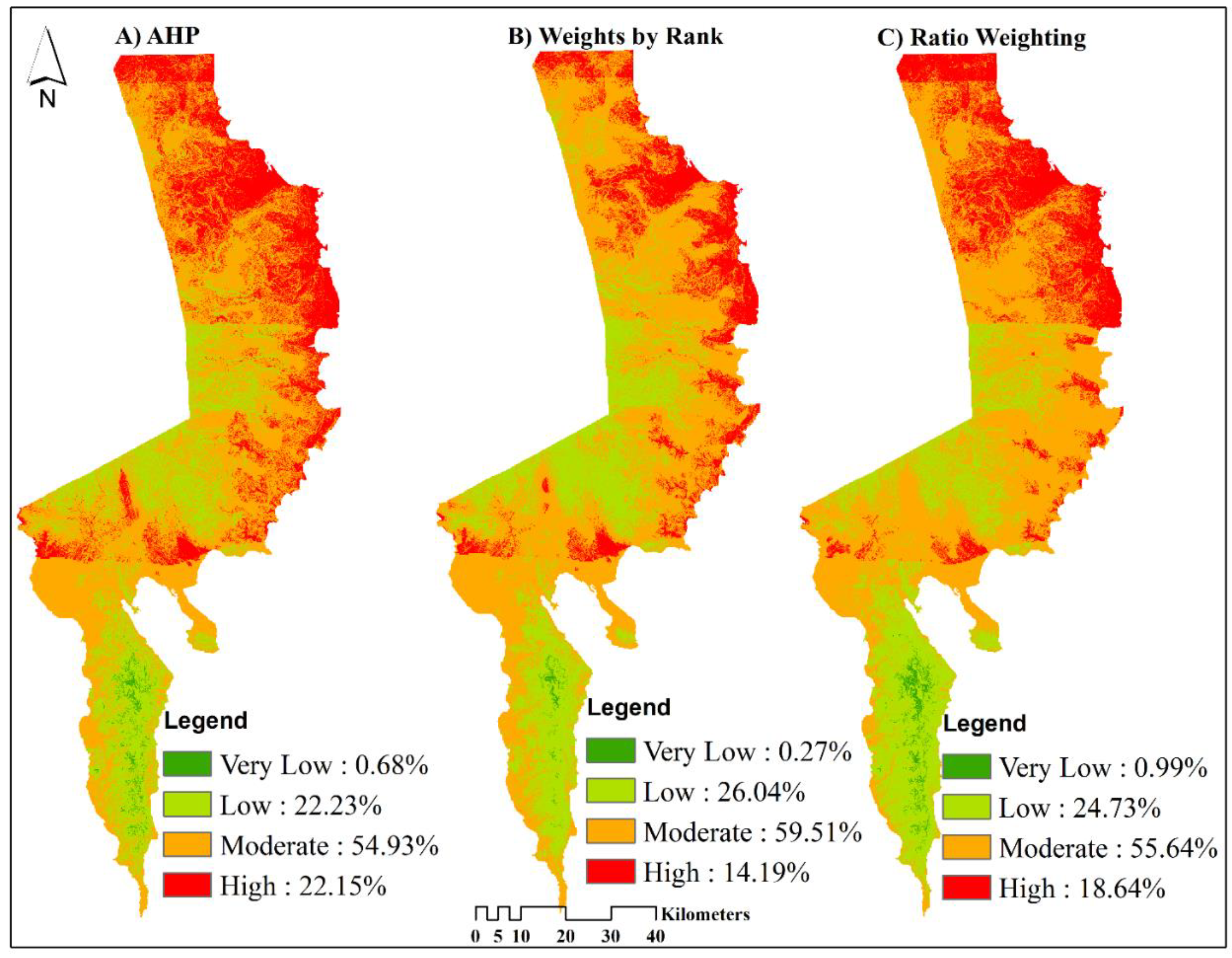
Finally, the HI obtained by the three models, AHP, WR and RW, was further processed using a weighted overlay analysis in ArcGIS. The results of weighted overlay analysis were classified using equal interval into four levels such as very low, low, moderate and high.
4.5. Validation
Super Typhoon Bopha was considered as one of the world’s damaging storms in 2012. Bopha entered the Philippine Area of Responsibility (PAR) as a rapidly intensified Category 5 Super Typhoon and made its landfall at Baganga, Davao Oriental, of 4 December 2012. It has reached an average speed of 185 kph and gusts reaching 210 kph. Typhoon Pablo, as what Typhoon Bopha is called in the Philippines, was the most powerful storm to have hit the island of Mindanao, southern Philippines, in more than 100 years of recorded storms [
60]. Its torrential rains generated massive debris flow in the Mayo River watershed in the Andap village in New Bataan municipality, causing some areas to be buried under a rubble as thick as 9 m and killing 566 people [
60]. Moreover, it was also revealed that a storm surge with a height of approximately 1 m has reached a distance of 500 m inland away from the coastline [
12]. Unfortunately, the government has no accounts in recording the flooded areas during the said event.
Due to the hazards caused by storm surge, storm surge prediction and forecasting currently is actually progressing. In fact, in a study conducted by Ross, et al. [
60] regarding the projected susceptibility to storm surge modeling using historical records from Philippine Atmospheric, Geophysical and Astronomical Services Administration (PAGASA), it showed that there was a storm surge event as high as 3.66 m. The said storm surge happened in the city of Bislig, located about 60 km from the northern coastal boundary of the Davao Oriental province. Hence, to address such scenarios, this study was conducted using a GPS-based field survey to determine the flooded areas during Typhoon Bopha.
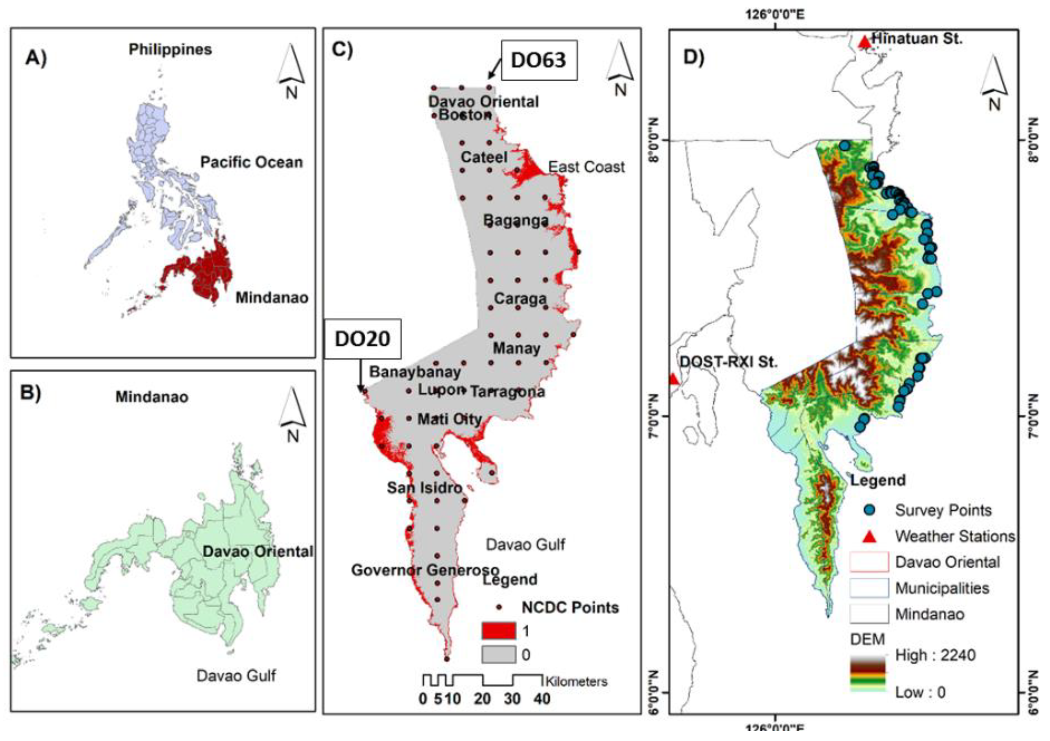
In order to validate the resulting flood-prone areas by the AHP, WR and RW methods, a GPS-based field survey to local people was carried out along the east coast of Davao Oriental to investigate ground true flooded points using historical flooding events. This survey was carried out to determine the flooded area during the Typhoon Bopha. It is to note that the field survey was also not carried out in the municipalities located near the Davao Gulf thus, the points do not cover all barangays specified in the study area. Hence, only 70 ground truthing points were collected and were used for performance evaluation (see
Figure 1D for the locations and Supplementary Material 3 for the survey result).
The performance evaluation was done using the accuracy assessment of the flood classification. One of the commonly used methods is to apply a confusion matrix or error matrix. This method can be used to compute several assessment elements such as overall accuracy (ACC), true positive rate (TPR), true negative rate (TNR), false positive rate (FPR) and false negative rate (FNR) using the Equations (11)–(15), respectively.
where P, N, TP, TN, FP and FN are condition positive, condition negative, true positive, true negative, false positive and false negative, respectively.
To evaluate the performance, an accuracy assessment was performed using the confusion matrix, and it was calculated based on the 70 ground points collected from the field survey. Elevations were extracted from these truthing points, and it showed that it is in the range between 10 m and 20 m above mean sea level. After spatially interpolating the points, it was identified that all areas in Davao Oriental that belongs to the below 20 m elevation were considered as susceptible flood-prone areas.
Based on the survey, a resulting map was created (as seen in
Figure 1C) and was overlaid with the prediction maps obtained by the AHP, RW and WR methods to compare and assess the accuracy of the prediction maps. In the accuracy assessment, the TP and FP are the numbers of pixels correctly classified and the numbers of pixels mistakenly classified, respectively. With this, the results showed that the number of correctly predicted pixels by the model (TP) are plotted to the number of incorrect predicted pixels (FP), as illustrated in
Table 5 and
Figure 5 , indicating that the AHP-based flood area is truly flooded in the ground truthing-based result.
Data scarcity and sparsity are the main problems solved in this approach. In this paper, data scarcity means limited historical flood events, or the recorded floods are limited as compared to the amount needed in the validation of the model (see
Figure 1D). Moreover, as shown in
Figure 1D, the survey data of flood are not evenly distributed (i.e., sparsity) to the study area. In this study, the flood data used was derived from the flooding caused by typhoon Bopha and did not cover all flood events happened in Davao Oriental. This approach has uncertainty and limitation, same with other hydrological modeling. Fortunately, the GIS-based flood validation approach is a good start for the researcher to conduct flood susceptibility mapping in data-scarce and sparse region.


