Identification of Hydrological Models for Enhanced Ensemble Reservoir Inflow Forecasting in a Large Complex Prairie Watershed


Abstract
1. Introduction
- Only a few studies were conducted on large and complex Prairie watersheds,
- Only a lumped model or a distributed model was used independently, for hydrological forecasting study. Alternatively, in some cases, the multi-models were only a collection of lumped conceptual models,
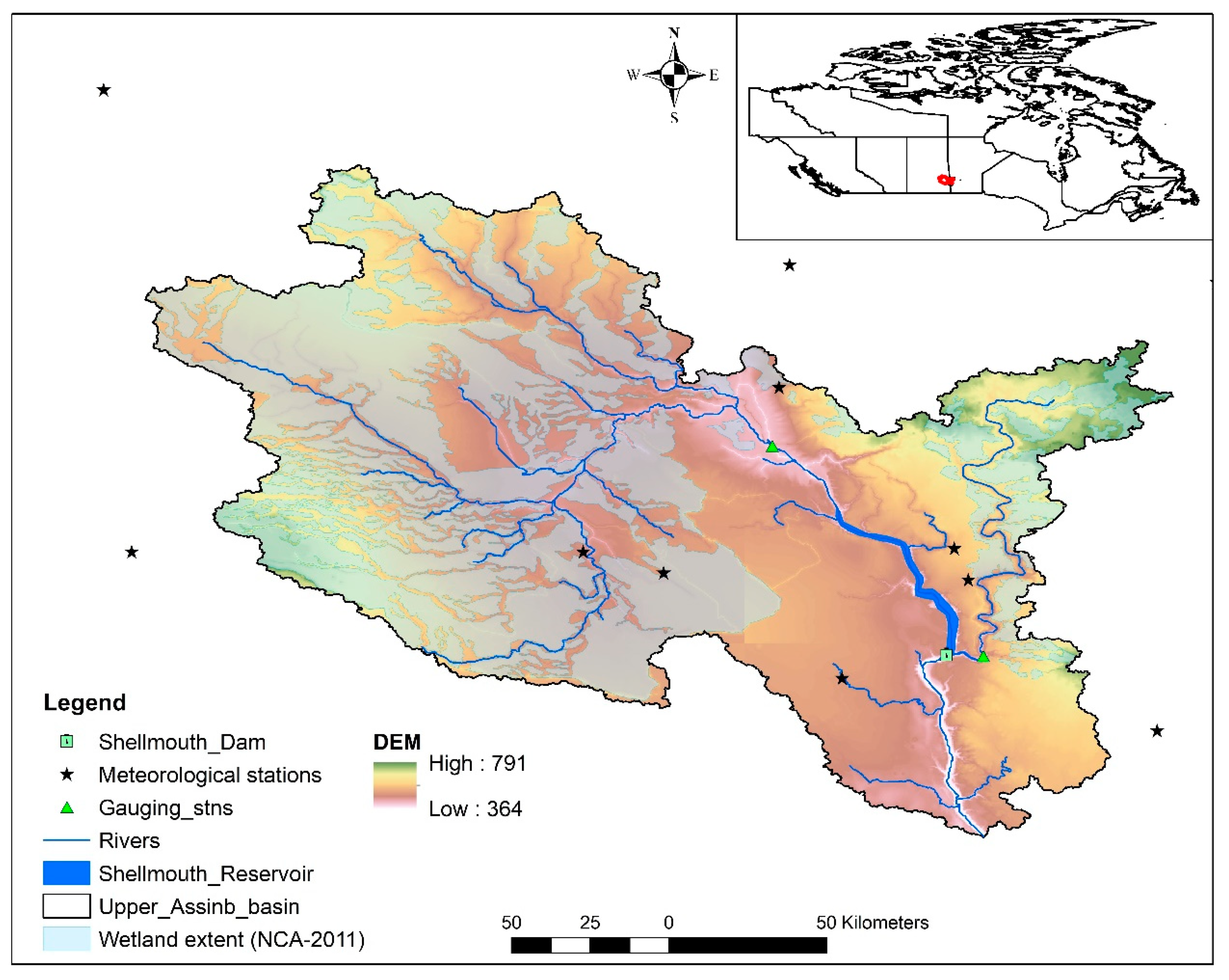
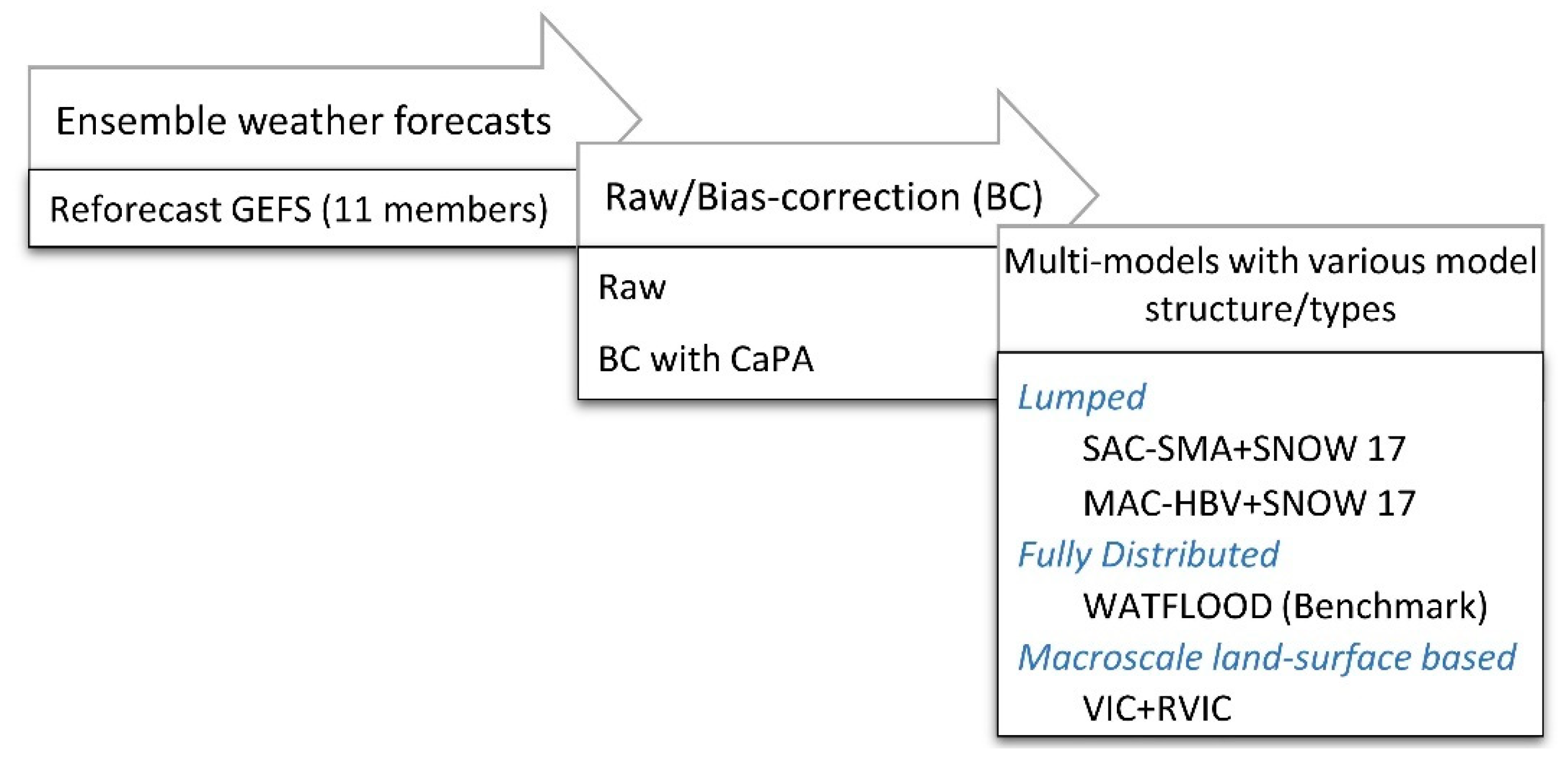
- Identification of best hydrological model was usually based on historical meteorological or in some cases, deterministic weather forecast inputs. Evaluation and comparison of models based on raw and bias-corrected ensemble precipitation forecasts were not studied. As such, the objective of this research is designed to address these limitations and identify the best hydrological model from diverse multi-models for short- and medium-range flood forecasting in a Canadian Prairie watershed. In this study, four structurally varied hydrological models were set up in order to simulate and forecast inflows to the Shelmouth Reservoir, which is located in Upper Assiniboine River Basin. A mixture of two lumped, one distributed and one macroscale land surface models were used in this research. In forecast mode, bias-corrected precipitation from second-generation Global Ensemble Forecast System (GEFS v2) reforecasts was fed into the four models in order to evaluate the reliability, skill, and overall forecast performance of the ensemble reservoir inflows.
2. Materials
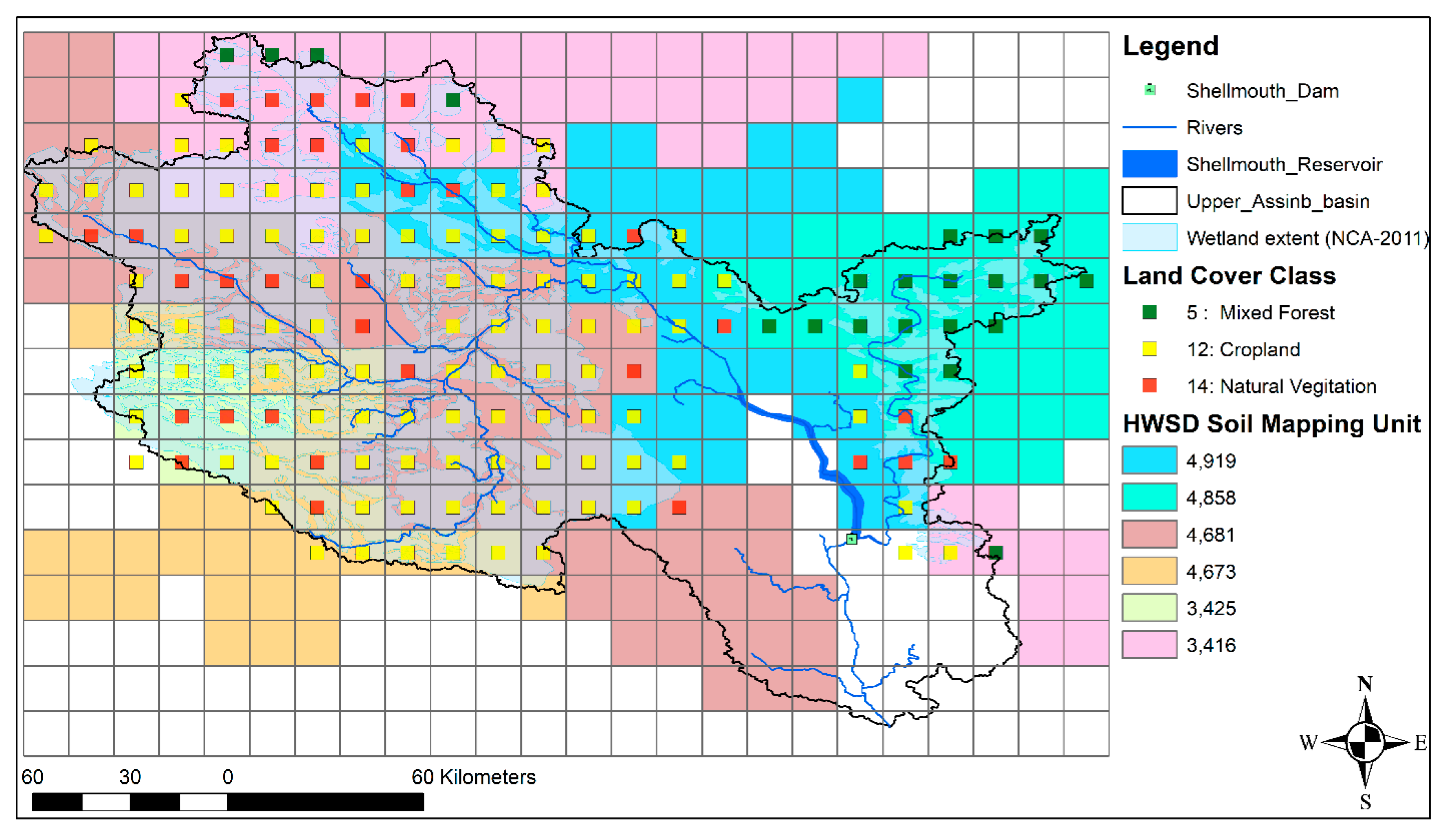
2.1. Study Area
2.2. Data
2.2.1. Ensemble Weather Forecasts
2.2.2. Observed Data
2.2.3. Reservoir Inflow
3. Methods
3.1. Hydrological Models
3.2. Calibration and Validation
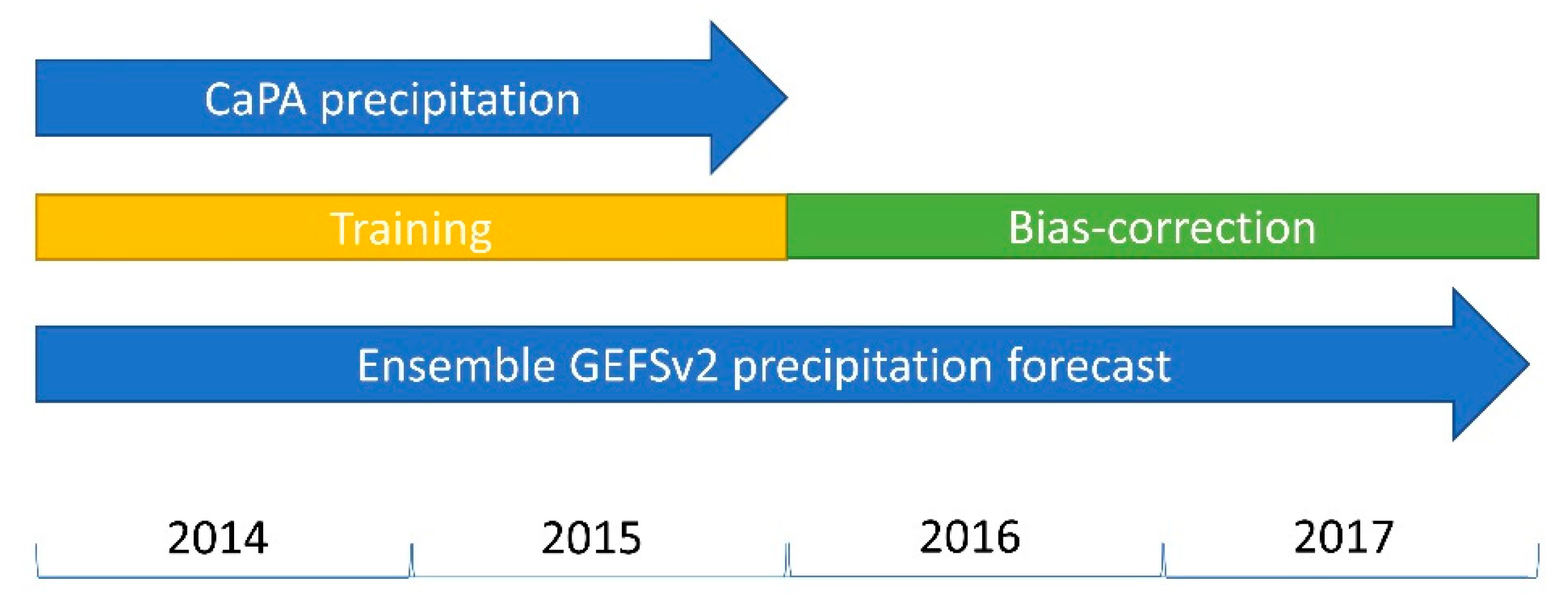
3.3. Bias-Correction
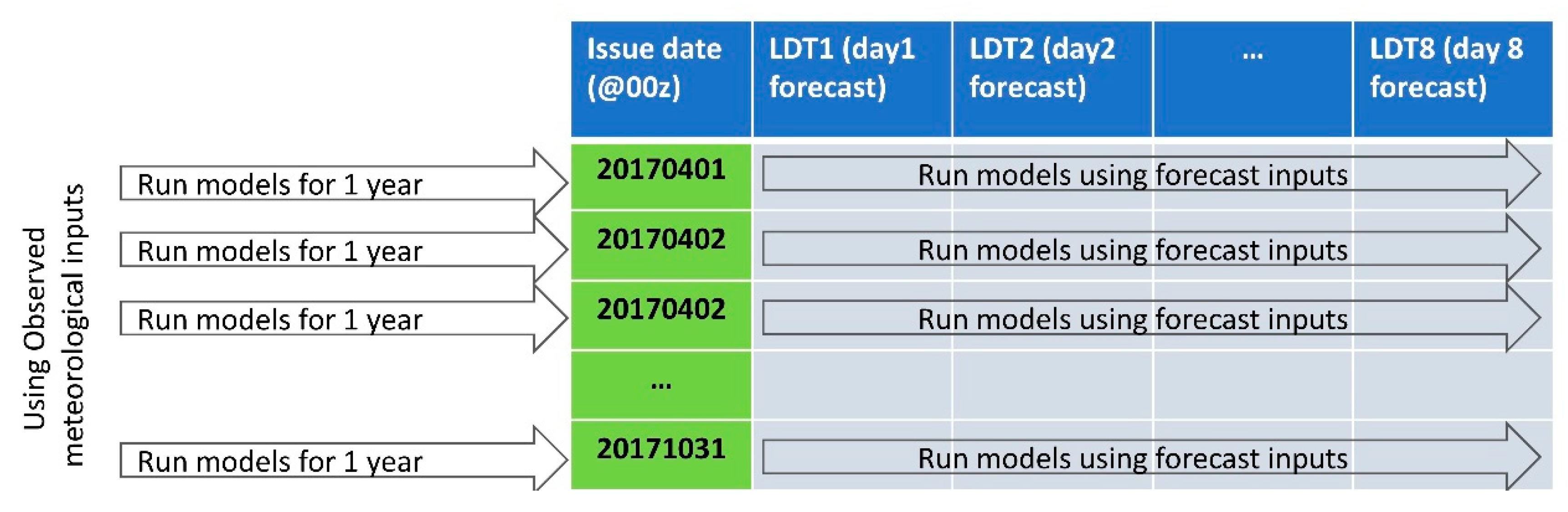
3.4. Hindcast Simulation (Model Update and Forecast)
3.5. Ensemble Forecast Verification
3.5.1. Mean Continuous Rank Probability Score () and Skill Score ()
3.5.2. Reliability Diagram
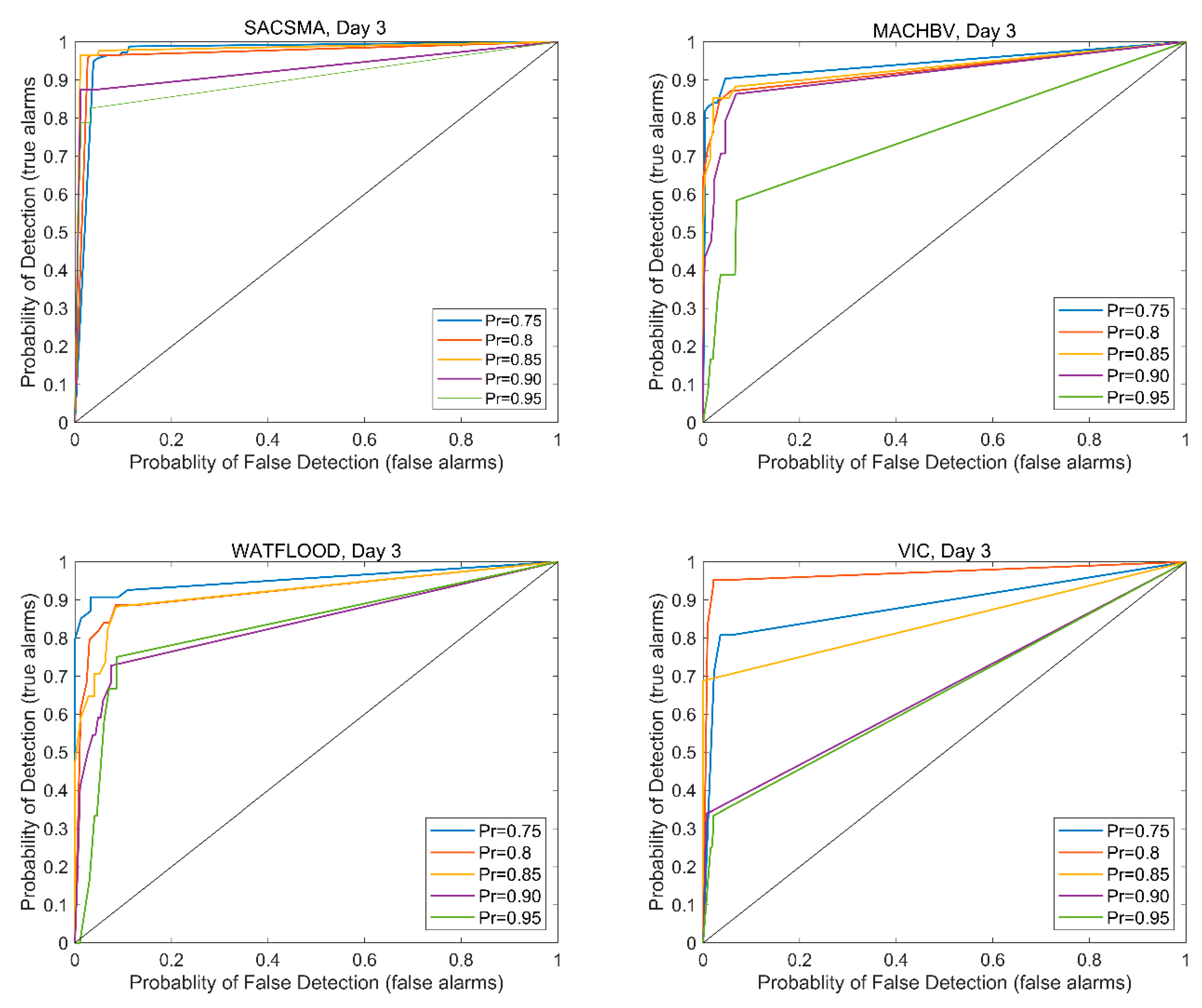
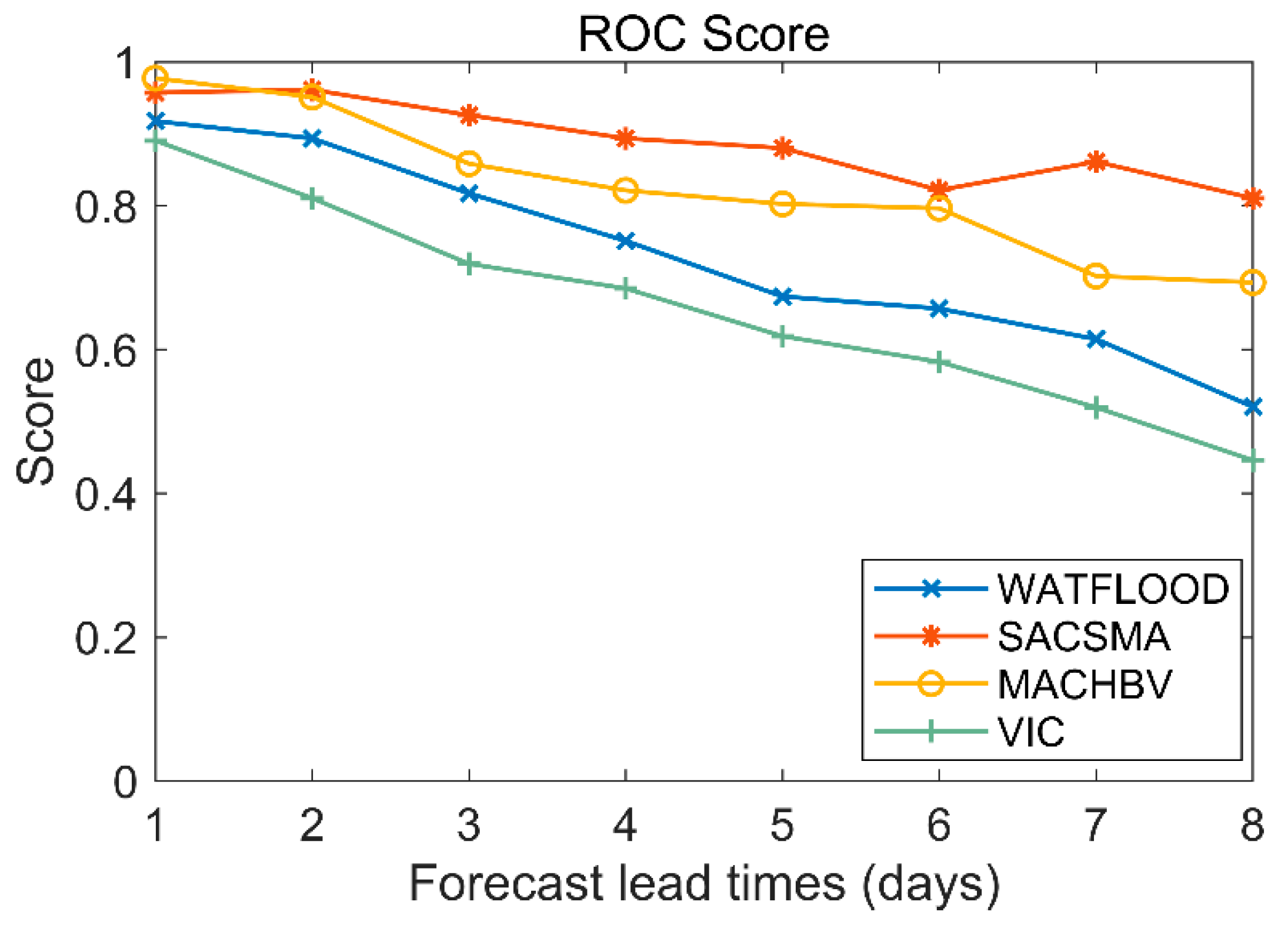
3.5.3. Relative Operating Characteristics (ROC) and Skill Score (ROC Score)
4. Results
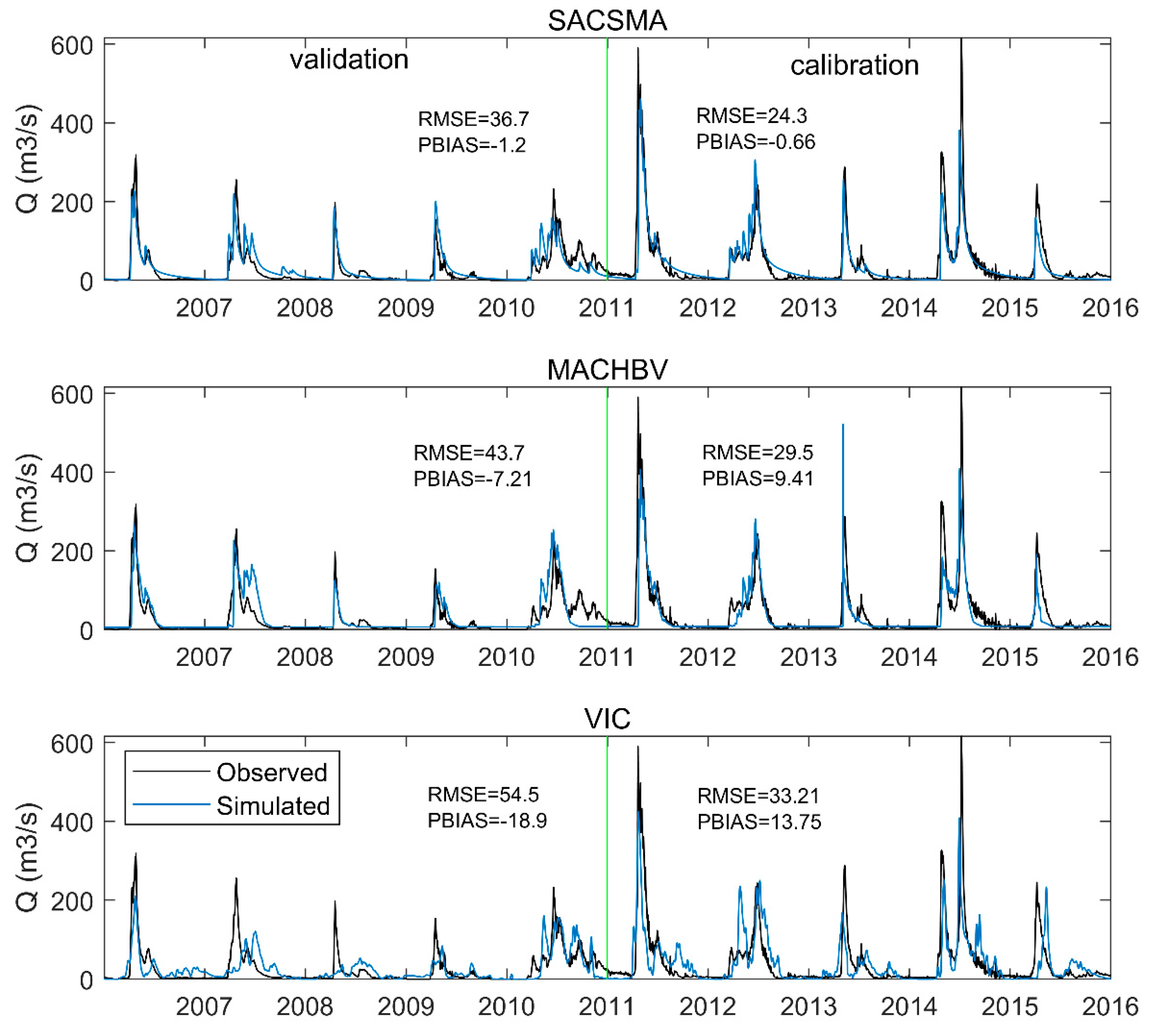
4.1. Calibration and Validation
4.2. Model Comparison in Forecast Mode
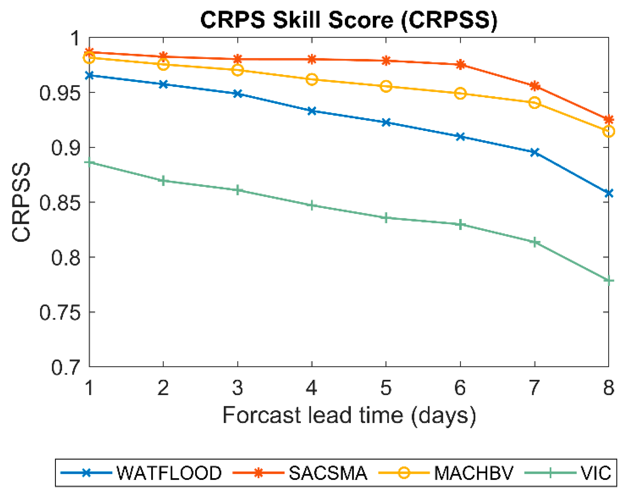
4.2.1. Overall Forecast Quality and Skill
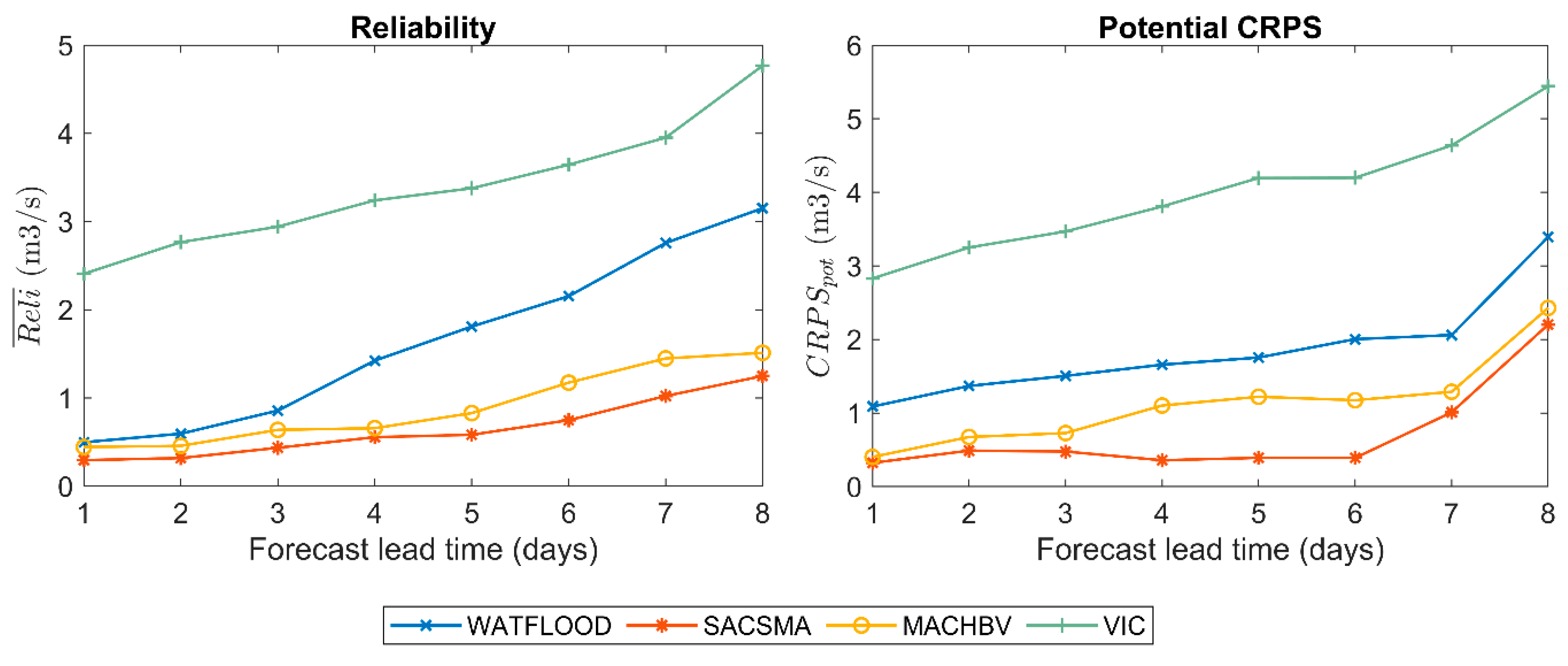
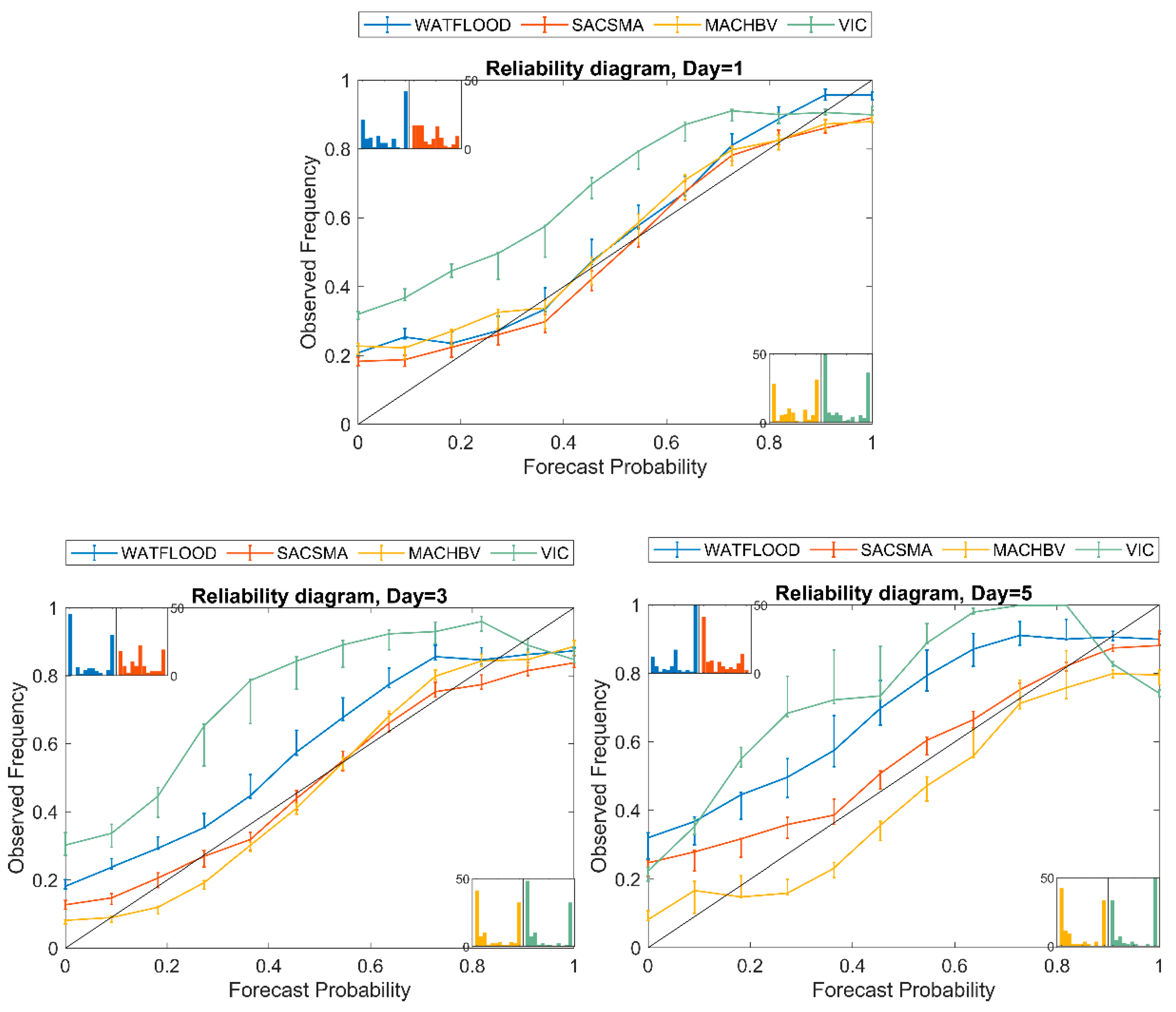
4.2.2. Reliability
4.2.3. Hit and False Alarm Rate Distribution
5. Conclusions and Discussion
Author Contributions
Funding
Acknowledgments
Conflicts of Interest
Appendix A. Brief Description of the Calibration of Models
Appendix A.1. SNOW17
- (i)
- The mean area observed precipitation time series obtained by Theisen Polygon method
- (ii)
- The mean area observed temperature time series obtained by Theisen Polygon method
- (iii)
- The average elevation of the catchment
- (iv)
- The latitude of the centroid of the catchment

| No | Parameters | Description | Unit | Ranges |
|---|---|---|---|---|
| 1 | SCF | Snowfall correction factor | – | 0.4–1.6 |
| 2 | MFMAX | Maximum melt factor during non-rain periods considered to occur on June 21 | mm/6 h/°C | 0.5–2.0 |
| 3 | MFMIN | Minimum melt factor during non-rain periods considered to occur on December 21 | mm/6 h/°C | 0.05–0.5 |
| 4 | UADJ | The average wind function during rain-on-snow periods | mm/mb/°C | 0.03–0.2 |
| 5 | NMF | Maximum negative melt factor | mm/6 h/°C | 0.05–0.50 |
| 6 | MBASE | Base temperature for non-rain melt factor above which melt typically occurs | °C | 0–2.0 |
| 7 | PXTEMP1 | Lower Limit Temperature dividing tranistion from snow, if temp is less than or equal to pxtemp1, all precip is snow. Otherwise it is mixed linearly | °C | −2.0 to 0 |
| 7 | PXTEMP2 | Upper Limit Temperature dividing tranistion from snow, if temp is greater than or equal to pxtemp2, all precip is rain. Otherwise it is mixed linearly | °C | 1 to 3.0 |
| 8 | PLWHC | percent liquid water holding capacity of the snow pack | – | 0.02–0.3 |
| 9 | DAYGM | Daily melt at snow–soil interface | mm/day | 0–0.3 |
| 10 | TIPM | Antecedent snow temperature index | – | 0.1–0.2 |
Appendix A.2. SACSMA
- (i)
- Outflow (rain plus snowmelt) from SNOW17
- (ii)
- The catchment area of the basin
- (iii)
- Observed catchment outflow estimated by calculated reservoir inflow
| No | Parameters | Description | Unit | Ranges |
|---|---|---|---|---|
| 1 | UZTWM | Upper zone tension water maximum storage | [mm] | 1–150 |
| 2 | UZFWM | Upper zone free water maximum storage | [mm] | 1–150 |
| 3 | LZTWM | Lower zone tension water maximum storage | [mm] | 1–500 |
| 4 | LZFPM | Lower zone free water primary maximum storage | [mm] | 1–1000 |
| 5 | LZFSM | Lower zone free water supplemental maximum storage | [mm] | 1–1000 |
| 6 | ADIMP | Additional impervious area | [-] | 0.0–0.4 |
| 7 | UZK | Upper zone free water lateral depletion rate | [day−1] | 0.1–0.5 |
| 8 | LZPK | Lower zone primary free water depletion rate | [day−1] | 0.0001–0.025 |
| 9 | LZSK | Lower zone supplemental free water depletion rate | [day−1] | 0.01–0.25 |
| 10 | ZPERC | Maximum percolation rate | [-] | 1–250 |
| 11 | REXP | Exponent of the percolation equation [-] | [-] | 1–5.0 |
| 12 | PCTIM | Impervious fraction of the watershed area | [-] | 0.0–0.1 |
| 13 | PFREE | fraction percolating from upper to lower zone free water Storage | [-] | 0.0–0.6 |
| 14 | athorn | A constant for Thornthwaite’s equation | [-] | 0.1–0.3 |
| 15 | Rq | Routing Coefficient | [-] | 0.0–1 |
Appendix A.3. MACHBV
- (i)
- Outflow (rain plus snowmelt) from SNOW17
- (ii)
- The catchment area of the basin
- (iii)
- Observed catchment outflow estimated by calculated reservoir inflow
| No | Parameters | Description | Unit | Ranges |
|---|---|---|---|---|
| 1 | athorn | A constant for Thornthwaite’s equation | [-] | 0.1–0.3 |
| 2 | fc | Maximum soil box water content | [mm] | 50–800 |
| 3 | lp | Limit for potential evaporation | [mm/mm] | 0.1 × fc–0.9 × fc |
| 4 | beta | A non-linear parameter controlling runoff generation | [-] | 1–10 |
| 5 | K0 | Flow recession coefficient in an upper soil reservoir | [days] | 1–30 |
| 6 | lsuz | A threshold value used to control response routing on an upper soil reservoir | [mm] | 1–100 |
| 7 | K1 | Flow recession coefficient in an upper soil reservoir | [days] | 2.5–100 |
| 8 | cperc | A constant percolation rate parameter | [mm/day] | 0.01–6 |
| 9 | K2 | Flow recession coefficient in a lower soil reservoir | [days] | 20–1000 |
| 10 | maxbas | A triangle weighting function for modelling a channel routing routine | [days] | 1–20 |
| 11 | rcr | Rainfall correction factor | [-] | 0.5–1.5 |
| 12 | a1 | An exponent in relation between outflow and storage representing non-linearity of storage – discharge relationship of lower reservoir | [-] | 0.5–20 |
Appendix A.4. VIC
- (i)
- Average daily gridded interpolated precipitation data from the ground network,
- (ii)
- Daily gridded minimum, and maximum temperature data from ANUSPLIN,
- (iii)
- Average daily wind speed from the Global Environmental Multiscale (GEM) model.
- (i)
- Digital elevation model for SNOW elevation bands and flow direction computation
- (ii)
- Land cover data from Moderate Resolution Imaging Spectroradiometer (MODIS) Land Cover Type (MCD12Q1) Version 6 data product
- (iii)
- Soil data from FAO’s Harmonized World Soil Database (HWSD) V 1.2
- (i)
- Snow: Rain-snow partitioning, snow accumulation, and melting are simulated at a sub-grid level using temperature index method lapsed through the Elevation (SNOW) bands.
- (ii)
- Evaporation: is simulated at each elevation band and land cover type using Penman-Monteith Approach.

| No | Notation | Range | Unit | Definition |
|---|---|---|---|---|
| Soil parameters | ||||
| 1 | b | 10−5–0.4 | - | Variable infiltration curve parameter |
| 2 | Ds | 10−3–1 | - | Fraction of Dsmax where non-linear baseflow begins |
| 3 | Dm | 0.1–30 | mm/day | Maximum velocity of baseflow |
| 4 | Ws | 0.5–1 | - | Fraction of maximum soil moisture where non-linear baseflow occurs |
| 5 | s2 | 0.3–1.5 | m | Thickness of middle soil moisture layer |
| 6 | s3 | 0.3–1.5 | m | Thickness of bottom soil moisture layer |
| Wetland parameters | ||||
| 7 | bmin_depth | 0.01–0.3 | m | Lake depth below which channel outflow is 0. |
| 8 | wfrac | 0.001–0.05 | - | Width of lake outlet, as a fraction of the lake perimeter |
| 9 | depth_in | 0.01–0.3 | m | Initial lake depth |
| 10 | rpercent | 0.1–1 | - | Fraction of grid cell runoff that enters lake (instead of going directly to channel network) |
| 11 | lake_depth | 0.1–1.5 | m | Maximum allowable depth of lake |
| Routing parameters | ||||
| 12 | Vl | 0.5–3 | m/s | Flow/Wave velocity |
| 13 | Df | 200–4000 | m2/s | Flow diffusion |
References
- Fang, X.; Minke, A.; Pomeroy, J.; Brown, T.; Westbrook, C.; Guo, X.; Guangul, S. A Review of Canadian Prairie Hydrology: Principles, Modelling and Response to Land Use and Drainage Change, Centre for Hydrology Report #2, Version 2; University of Saskatchewan: Saskatoon, SK, Canada, 2007. [Google Scholar]
- Armstrong, R.N.; Pomeroy, J.W.; Martz, L.W. Evaluation of Three Evaporation Estimation Methods in a Canadian Prairie Landscape Robert. Hydrol. Process. 2008, 22, 2801–2815. [Google Scholar] [CrossRef]
- Fang, X.; Pomeroy, J.W.; Westbrook, C.J.; Guo, X.; Minke, A.G.; Brown, T. Prediction of Snowmelt Derived Streamflow in a Wetland Dominated Prairie Basin. Hydrol. Earth Syst. Sci. 2010, 14, 1–16. [Google Scholar] [CrossRef]
- Hayashi, M.; Van Der Kamp, G. Simple Equations to Represent the Volume-Area-Depth Relations of Shallow Wetlands in Small Topographic Depressions. J. Hydrol. 2000, 237, 74–85. [Google Scholar] [CrossRef]
- Shook, K.; Pomeroy, J.; van der Kamp, G. The Transformation of Frequency Distributions of Winter Precipitation to Spring Streamflow Probabilities in Cold Regions; Case Studies from the Canadian Prairies. J. Hydrol. 2015, 521, 394–409. [Google Scholar] [CrossRef]
- Eum, H.I.; Dibike, Y.; Prowse, T. Climate-Induced Alteration of Hydrologic Indicators in the Athabasca River Basin, Alberta, Canada. J. Hydrol. 2017, 544, 327–342. [Google Scholar] [CrossRef]
- Hedstrom, N.R.; Granger, R.J.; Pomeroy, J.W.; Gray, D.M. Enhanced Indicators of Land Use Change and Climate Variability Impacts on Prairie Hydrology Using the Cold Regions Hydrological Model. In Proceedings of the 58th Eastern Snow Conference, Ottawa, ON, Canada, 17–19 May 2001; pp. 262–275. [Google Scholar]
- Pattison-Williams, J.K.; Pomeroy, J.W.; Badiou, P.; Gabor, S. Analysis Wetlands, Flood Control and Ecosystem Services in the Smith Creek Drainage Basin: A Case Study in Saskatchewan, Canada. Ecol. Econ. J. 2018, 147, 36–47. [Google Scholar] [CrossRef]
- Pomeroy, J.W.; Gray, D.M.; Brown, T.; Hedstrom, N.R.; Quinton, W.L.; Granger, R.J.; Carey, S.K. The Cold Regions Hydrological Model: A Platform for Basing Process Representation and Model Structure on Physical Evidence. Hydrol. Process. 2007, 21, 2650–2667. [Google Scholar] [CrossRef]
- Mekonnen, M.A.; Wheater, H.S.; Ireson, A.M.; Spence, C.; Davison, B.; Pietroniro, A. Towards an Improved Land Surface Scheme for Prairie Landscapes. J. Hydrol. 2014, 511, 105–116. [Google Scholar] [CrossRef]
- Gray, D.M.; Landine, P.G. An Energy-Budget Snowmelt Model for the Canadian Prairies. Can. J. Earth Sci. 1988, 25, 1292–1303. [Google Scholar] [CrossRef]
- Shook, K.; Pomeroy, J.W.; Spence, C.; Boychuk, L. Storage Dynamics Simulations in Prairie Wetland Hydrology Models: Evaluation and Parameterization. Hydrol. Process. 2013, 27, 1875–1889. [Google Scholar] [CrossRef]
- Evenson, G.R.; Golden, H.E.; Lane, C.R.; D’Amico, E. An Improved Representation of Geographically Isolated Wetlands in a Watershed-Scale Hydrologic Model. Hydrol. Process. 2016, 30, 4168–4184. [Google Scholar] [CrossRef]
- Brochero, D.; Anctil, F.; Gagné, C. Simplifying a Hydrological Ensemble Prediction System with a Backward Greedy Selection of Members—Part 2: Generalization in Time and Space. Hydrol. Earth Syst. Sci. 2011, 15, 3327–3341. [Google Scholar] [CrossRef]
- Ajami, N.K.; Duan, Q.; Gao, X.; Sorooshian, S. Multimodel Combination Techniques for Analysis of Hydrological Simulations: Application to Distributed Model Intercomparison Project Results. J. Hydrometeorol. 2006, 7, 755–768. [Google Scholar] [CrossRef]
- Seiller, G.; Anctil, F.; Perrin, C. Multimodel Evaluation of Twenty Lumped Hydrological Models under Contrasted Climate Conditions. Hydrol. Earth Syst. Sci. 2012, 16, 1171–1189. [Google Scholar] [CrossRef]
- Velázquez, J.A.; Anctil, F.; Perrin, C. Performance and Reliability of Multimodel Hydrological Ensemble Simulations Based on Seventeen Lumped Models and a Thousand Catchments. Hydrol. Earth Syst. Sci. 2010, 14, 2303–2317. [Google Scholar] [CrossRef]
- Velázquez, J.A.; Anctil, F.; Ramos, M.H.; Perrin, C. Can a Multi-Model Approach Improve Hydrological Ensemble Forecasting? A Study on 29 French Catchments Using 16 Hydrological Model Structures. Adv. Geosci. 2011, 29, 33–42. [Google Scholar] [CrossRef]
- Viney, N.R.; Bormann, H.; Breuer, L.; Bronstert, A.; Croke, B.F.W.; Frede, H.; Gräff, T.; Hubrechts, L.; Huisman, J.A.; Jakeman, A.J.; et al. Assessing the Impact of Land Use Change on Hydrology by Ensemble Modelling (LUCHEM) II: Ensemble Combinations and Predictions. Adv. Water Resour. 2009, 32, 147–158. [Google Scholar] [CrossRef]
- Seiller, G.; Anctil, F.; Roy, R. Design and Experimentation of an Empirical Multistructure Framework for Accurate, Sharp and Reliable Hydrological Ensembles. J. Hydrol. 2017, 552, 313–340. [Google Scholar] [CrossRef]
- Thiboult, A.; Anctil, F.; Boucher, M.A. Accounting for Three Sources of Uncertainty in Ensemble Hydrological Forecasting. Hydrol. Earth Syst. Sci. 2016, 20, 1809–1825. [Google Scholar] [CrossRef]
- Antonetti, M.; Horat, C.; Sideris, I.V.; Zappa, M. Ensemble Flood Forecasting Considering Dominant Runoff Processes: I. Setup and Application to Nested Basins (Emme, Switzerland). Nat. Hazards Earth Syst. Sci. Discuss. 2018, 5194, 1–29. [Google Scholar] [CrossRef]
- Alfieri, L.; Pappenberger, F.; Wetterhall, F.; Haiden, T.; Richardson, D.; Salamon, P. Evaluation of Ensemble Streamflow Predictions in Europe. J. Hydrol. 2014, 517, 913–922. [Google Scholar] [CrossRef]
- Calvetti, L.; Pereira Filho, A.J. Ensemble Hydrometeorological Forecasts Using WRF Hourly QPF and Topmodel for a Middle Watershed. Adv. Meteorol. 2014, 2014. [Google Scholar] [CrossRef]
- Fan, F.M.; Schwanenberg, D.; Kuwajima, J.; Assis, A. Ensemble Streamflow Predictions in the Três Marias Basin, Brazil. In Proceedings of the EGU General Assembly Conference, Vienna, Austria, 27 April–2 May 2014; Volume 16, p. 14191. [Google Scholar]
- Liechti, K.; Zappa, M.; Fundel, F.; Germann, U. Probabilistic Evaluation of Ensemble Discharge Nowcasts in Two Nested Alpine Basins Prone to Flash Floods. Hydrol. Process. 2013, 27, 5–17. [Google Scholar] [CrossRef]
- Pietroniro, A.; Fortin, V.; Kouwen, N.; Neal, C.; Turcotte, R.; Davison, B.; Verseghy, D.; Soulis, E.D.; Caldwell, R.; Evora, N.; et al. Development of the MESH Modelling System for Hydrological Ensemble Forecasting of the Laurentian Great Lakes at the Regional Scale. Hydrol. Earth Syst. Sci. 2007, 11, 1279–1294. [Google Scholar] [CrossRef]
- Thiemig, V.; Pappenberger, F.; Thielen, J.; Gadain, H.; de Roo, A.; Bodis, K.; Del Medico, M.; Muthusi, F. Ensemble Flood Forecasting in Africa: A Feasibility Study in the Juba-Shabelle River Basin. Atmos. Sci. Lett. 2010, 11, 123–131. [Google Scholar] [CrossRef]
- Zsótér, E.; Pappenberger, F.; Smith, P.; Emerton, R.E.; Dutra, E.; Wetterhall, F.; Richardson, D.; Bogner, K.; Balsamo, G. Building a Multimodel Flood Prediction System with the TIGGE Archive. J. Hydrometeorol. 2016, 17, 2923–2940. [Google Scholar] [CrossRef]
- Fan, F.M.; Collischonn, W.; Meller, A.; Botelho, L.C.M. Ensemble Streamflow Forecasting Experiments in a Tropical Basin: The São Francisco River Case Study. J. Hydrol. 2014, 519, 2906–2919. [Google Scholar] [CrossRef]
- Fan, F.M.; Schwanenberg, D.; Collischonn, W.; Weerts, A. Verification of Inflow into Hydropower Reservoirs Using Ensemble Forecasts of the TIGGE Database for Large Scale Basins in Brazil. J. Hydrol. Reg. Stud. 2015, 4, 196–227. [Google Scholar] [CrossRef]
- Abaza, M.; Anctil, F.; Fortin, V.; Turcotte, R. A Comparison of the Canadian Global and Regional Meteorological Ensemble Prediction Systems for Short-Term Hydrological Forecasting. Mon. Weather Rev. 2013, 141, 3462–3476. [Google Scholar] [CrossRef]
- Jasper, K.; Gurtz, J.; Lang, H. Advanced Flood Forecasting in Alpine Watersheds by Coupling Meteorological Observations and Forecasts with a Distributed Hydrological Model. J. Hydrol. 2002, 267, 40–52. [Google Scholar] [CrossRef]
- Achleitner, S.; Schöber, J.; Rinderer, M.; Leonhardt, G.; Schöberl, F.; Kirnbauer, R.; Schönlaub, H. Analyzing the Operational Performance of the Hydrological Models in an Alpine Flood Forecasting System. J. Hydrol. 2012, 412–413, 90–100. [Google Scholar] [CrossRef]
- De Roo, A.P.J.; Gouweleeuw, B.; Thielen, J.; Bartholmes, J.; Bongioannini-Cerlini, P.; Todini, E.; Bates, P.D.; Horritt, M.; Hunter, N.; Beven, K.; et al. Development of a European Flood Forecasting System. Int. J. River Basin Manag. 2003, 1, 49–59. [Google Scholar] [CrossRef]
- Pappenberger, F.; Bartholmes, J.; Thielen, J.; Cloke, H.L.; Buizza, R.; de Roo, A. New Dimensions in Early Flood Warning across the Globe Using Grand-Ensemble Weather Predictions. Geophys. Res. Lett. 2008, 35, L10404. [Google Scholar] [CrossRef]
- Demargne, J.; Wu, L.; Regonda, S.K.; Brown, J.D.; Lee, H.; He, M.; Seo, D.J.; Hartman, R.; Herr, H.D.; Fresch, M.; et al. The Science of NOAA’s Operational Hydrologic Ensemble Forecast Service. Bull. Am. Meteorol. Soc. 2014, 95, 79–98. [Google Scholar] [CrossRef]
- Maxey, R.; Cranston, M.; Tavendale, A.; Buchanan, P. The Use of Deterministic and Probabilistic Forecasting in Countrywide Flood Guidance in Scotland. Hydrol. Change World 2012, 1–7. [Google Scholar] [CrossRef]
- Unduche, F.; Tolossa, H.; Senbeta, D.; Zhu, E. Evaluation of Four Hydrological Models for Operational Flood Forecasting in a Canadian Prairie Watershed. Hydrol. Sci. J. 2018, 63, 1–17. [Google Scholar] [CrossRef]
- Hrachowitz, M.; Clark, M.P. HESS Opinions: The Complementary Merits of Competing Modelling Philosophies in Hydrology. Hydrol. Earth Syst. Sci. 2017, 21, 3953–3973. [Google Scholar] [CrossRef]
- Shrestha, R.R.; Dibike, Y.B.; Prowse, T.D. Modelling of Climate-Induced Hydrologic Changes in the Lake Winnipeg Watershed. J. Great Lakes Res. 2012, 38 (Suppl. S3), 83–94. [Google Scholar] [CrossRef]
- Hamill, T.M.; Bates, G.T.; Whitaker, J.S.; Murray, D.R.; Fiorino, M.; Galarneau, T.J.; Zhu, Y.; Lapenta, W. NOAA’s Second-Generation Global Medium-Range Ensemble Reforecast Dataset. Bull. Am. Meteorol. Soc. 2013, 94, 1553–1565. [Google Scholar] [CrossRef]
- Mahfouf, J.F.; Brasnett, B.; Gagnon, S. A Canadian Precipitation Analysis (CaPA) Project: Description and Preliminary Results. Atmos. Ocean 2007, 45, 1–17. [Google Scholar] [CrossRef]
- Anderson, E. Snow Accumulation and Ablation Model—SNOW-17; National Weather Service: Silver Spring, MD, USA, 2006. [CrossRef]
- Samuel, J.; Coulibaly, P.; Metcalfe, R.A. Estimation of Continuous Streamflow in Ontario Ungauged Basins: Comparison of Regionalization Methods. J. Hydrol. Eng. 2011, 16, 447–459. [Google Scholar] [CrossRef]
- Liang, X.; Lettenmaier, D.P.; Wood, E.F.; Burges, S.J. A Simple Hydrologically Based Model of Land Surface Water and Energy Fluxes for General Circulation Models. J. Geophys. Res. 1994, 99, 14415. [Google Scholar] [CrossRef]
- Dibike, Y.; Eum, H.-I.; Prowse, T. Modelling the Athabasca Watershed Snow Response to a Changing Climate. J. Hydrol. Reg. Stud. 2018, 15, 134–148. [Google Scholar] [CrossRef]
- Eum, H.I.; Dibike, Y.; Prowse, T. Uncertainty in Modelling the Hydrologic Responses of a Large Watershed: A Case Study of the Athabasca River Basin, Canada. Hydrol. Process. 2014, 28, 4272–4293. [Google Scholar] [CrossRef]
- Eum, H.I.; Dibike, Y.; Prowse, T.; Bonsal, B. Inter-Comparison of High-Resolution Gridded Climate Data Sets and Their Implication on Hydrological Model Simulation over the Athabasca Watershed, Canada. Hydrol. Process. 2014, 28, 4250–4271. [Google Scholar] [CrossRef]
- Kouwen, N. WATFLOOD: A Micro-Computer Based Flood Forecasting System Based on Real-Time Weather Radar. Can. Water Resour. J. 1988, 13, 62–77. [Google Scholar] [CrossRef]
- Haghnegahdar, A.; Tolson, B.A.; Davison, B.; Seglenieks, F.R.; Klyszejko, E.; Soulis, E.D.; Fortin, V.; Matott, L.S. Calibrating Environment Canada’s MESH Modelling System over the Great Lakes Basin. Atmos. Ocean 2014, 52, 281–293. [Google Scholar] [CrossRef]
- Newman, A.J.; Mizukami, N.; Clark, M.P.; Wood, A.W.; Nijssen, B.; Nearing, G.; Newman, A.J.; Mizukami, N.; Clark, M.P.; Wood, A.W.; et al. Benchmarking of a Physically Based Hydrologic Model. J. Hydrometeorol. 2017, 18, 2215–2225. [Google Scholar] [CrossRef]
- Hopkinson, R.F.; Mckenney, D.W.; Milewska, E.J.; Hutchinson, M.F.; Papadopol, P.; Vincent, A.L.A. Impact of Aligning Climatological Day on Gridding Daily Maximum-Minimum Temperature and Precipitation over Canada. J. Appl. Meteorol. Climatol. 2011, 50, 1654–1665. [Google Scholar] [CrossRef]
- Hutchinson, M.F.; McKenney, D.W.; Lawrence, K.; Pedlar, J.H.; Hopkinson, R.F.; Milewska, E.; Papadopol, P. Development and Testing of Canada-Wide Interpolated Spatial Models of Daily Minimum-Maximum Temperature and Precipitation for 1961-2003. J. Appl. Meteorol. Climatol. 2009, 48, 725–741. [Google Scholar] [CrossRef]
- Côté, J.; Desmarais, J.G.; Gravel, S.; Méthot, A.; Patoine, A.; Roch, M.; Staniforth, A. The Operational CMC-MRB Global Environmental Multiscale (GEM) Model. Part II: Results. Mon. Weather Rev. 1998, 126, 1397–1418. [Google Scholar] [CrossRef]
- Friedl, M.; Sulla-Menashe, D. MCD12Q1 MODIS/Terra+Aqua Land Cover Type Yearly L3 Global 500 m SIN Grid V006 [Data Set]; NASA EOSDIS Land Processes DAAC: Washington, DC, USA, 2015. [CrossRef]
- FAO; JRC; IIASA; ISRIC; ISS-CAS. Harmonized World Soil Database—Version 1.1; FAO: Rome, Italy; IIASA: Laxenburg, Austria, 2009. [Google Scholar]
- Hamman, J.; Nijssen, B.; Clark, E.; Matthews, D.; Veerman, B. UW-Hydro/RVIC: RVIC 1.1.1, v1.1.1. 2017. [CrossRef]
- Lohmann, D.; Nolte-Holube, R.; Raschke, E. A Large-Scale Horizontal Routing Model to Be Coupled to Land Surface Parametrization Schemes. Tellus Ser. A Dyn. Meteorol. Oceanogr. 1996, 48, 708–721. [Google Scholar] [CrossRef]
- Tolson, B.A.; Shoemaker, C.A. Dynamically Dimensioned Search Algorithm for Computationally Efficient Watershed Model Calibration. Water Resour. Res. 2007, 43, 1–16. [Google Scholar] [CrossRef]
- Ilampooranan, I.; Van Meter, K.J.; Basu, N.B. A Race against Time: Modeling Time Lags in Watershed Response. Water Resour. Res. 2019, 55, 3941–3959. [Google Scholar] [CrossRef]
- Aliyari, F.; Bailey, R.T.; Tasdighi, A.; Dozier, A.; Arabi, M.; Zeiler, K. Coupled SWAT-MODFLOW Model for Large-Scale Mixed Agro-Urban River Basins. Environ. Model. Softw. 2019, 115, 200–210. [Google Scholar] [CrossRef]
- Rokaya, P.; Wheater, H.; Lindenschmidt, K.E. Promoting Sustainable Ice-Jam Flood Management along the Peace River and Peace-Athabasca Delta. J. Water Resour. Plan. Manag. 2019, 145, 1–12. [Google Scholar] [CrossRef]
- Krogh, S.A.; Pomeroy, J.W. Impact of Future Climate and Vegetation on the Hydrology of an Arctic Headwater Basin at the Tundra-Taiga Transition. J. Hydrometeorol. 2019, 20, 197–215. [Google Scholar] [CrossRef]
- Sharma, S.; Siddique, R.; Reed, S.; Ahnert, P.; Mejia, A. Hydrological Model Diversity Enhances Streamflow Forecast Skill at Short- to Medium-Range Timescales. Water Resour. Res. 2019, 55, 1510–1530. [Google Scholar] [CrossRef]
- Lahmers, T.M.; Gupta, H.; Castro, C.L.; Gochis, D.J.; Yates, D.; Dugger, A.; Goodrich, D.; Hazenberg, P. the structure of the W. hydrologic model for semiarid environments. Enhancing the Structure of the WRF-Hydro Hydrologic Model for Semiarid Environments. J. Hydrometeorol. 2019, 20, 691–714. [Google Scholar] [CrossRef]
- Gupta, H.V.; Kling, H.; Yilmaz, K.K.; Martinez, G.F. Decomposition of the Mean Squared Error and NSE Performance Criteria: Implications for Improving Hydrological Modelling. J. Hydrol. 2009, 377, 80–91. [Google Scholar] [CrossRef]
- Coulibaly, P.; Anctil, F.; Bobée, B. Multivariate Reservoir Inflow Forecasting Using Temporal Neural Networks. J. Hydrol. Eng. 2001, 6, 367–376. [Google Scholar] [CrossRef]
- Amengual, A.; Homar, V.; Romero, R.; Alonso, S.; Ramis, C.; Amengual, A.; Homar, V.; Romero, R.; Alonso, S.; Ramis, C. A Statistical Adjustment of Regional Climate Model Outputs to Local Scales: Application to Platja de Palma, Spain. J. Clim. 2012, 25, 939–957. [Google Scholar] [CrossRef]
- Wilks, D. Statistical Methods in the Atmospheric Sciences, 2nd ed.; Acadamic Press: Cambridge, MA, USA, 2006; Volume 91. [Google Scholar]
- Hersbach, H. Decomposition of the Continuous Ranked Probability Score for Ensemble Prediction Systems. Weather Forecast. 2000, 15, 559–570. [Google Scholar] [CrossRef]
- Bradley, A.A.; Schwartz, S.S. Summary Verification Measures and Their Interpretation for Ensemble Forecasts. Mon. Weather Rev. 2011, 139, 3075–3089. [Google Scholar] [CrossRef]
- Muhammad, A.; Stadnyk, T.; Unduche, F.; Coulibaly, P.; Muhammad, A.; Stadnyk, T.A.; Unduche, F.; Coulibaly, P. Multi-Model Approaches for Improving Seasonal Ensemble Streamflow Prediction Scheme with Various Statistical Post-Processing Techniques in the Canadian Prairie Region. Water 2018, 10, 1604. [Google Scholar] [CrossRef]
- Pappenberger, F.; Ramos, M.H.; Cloke, H.L.; Wetterhall, F.; Alfieri, L.; Bogner, K.; Mueller, A.; Salamon, P. How Do I Know If My Forecasts Are Better? Using Benchmarks in Hydrological Ensemble Prediction. J. Hydrol. 2015, 522, 697–713. [Google Scholar] [CrossRef]
- Hsu, W.-R.; Murphy, A.H. The Attributes Diagram A Geometrical Framework for Assessing the Quality of Probability Forecasts. Int. J. Forecast. 1986, 2, 285–293. [Google Scholar] [CrossRef]
- Atger, F. The Skill of Ensemble Prediction Systems. Mon. Weather Rev. 1999, 127, 1941–1953. [Google Scholar] [CrossRef]
- Mason, S.J.; Graham, N.E. Areas beneath the Relative Operating Characteristics (ROC) and Relative Operating Levels (ROL) Curves: Statistical Significance and Interpretation. Q. J. R. Meteorol. Soc. 2002, 128, 2145–2166. [Google Scholar] [CrossRef]
- Brown, J.D.; Demargne, J.; Seo, D.J.; Liu, Y. The Ensemble Verification System (EVS): A Software Tool for Verifying Ensemble Forecasts of Hydrometeorological and Hydrologic Variables at Discrete Locations. Environ. Model. Softw. 2010, 25, 854–872. [Google Scholar] [CrossRef]
- Chang, H.-L.; Yang, S.-C.; Yuan, H.; Lin, P.-L.; Liou, Y.-C.; Chang, H.-L.; Yang, S.-C.; Yuan, H.; Lin, P.-L.; Liou, Y.-C. Analysis of the Relative Operating Characteristic and Economic Value Using the LAPS Ensemble Prediction System in Taiwan. Mon. Weather Rev. 2015, 143, 1833–1848. [Google Scholar] [CrossRef]
- Mason, S.J.; Graham, N.E. Conditional Probabilities, Relative Operating Characteristics, and Relative Operating Levels. Weather Forecast. 1999, 14, 713–725. [Google Scholar] [CrossRef]
- Yapo, P.O.; Gupta, H.V.; Sorooshian, S. Automatic Calibration of Conceptual Rainfall-Runoff Models: Sensitivity to Calibration Data. J. Hydrol. 1996, 181, 23–48. [Google Scholar] [CrossRef]
- Reed, S.; Koren, V.; Smith, M.; Zhang, Z.; Moreda, F.; Seo, D.J. Overall Distributed Model Intercomparison Project Results. J. Hydrol. 2004, 298, 27–60. [Google Scholar] [CrossRef]
- Duan, Q.; Schaake, J.; Andréassian, V.; Franks, S.; Goteti, G.; Gupta, H.V.; Gusev, Y.M.; Habets, F.; Hall, A.; Hay, L.; et al. Model Parameter Estimation Experiment (MOPEX): An Overview of Science Strategy and Major Results from the Second and Third Workshops. J. Hydrol. 2006, 320, 3–17. [Google Scholar] [CrossRef]
- Nasonova, O.N.; Gusev, Y.M. Can a Land Surface Model Simulate Runoff with the Same Accuracy as a Hydrological Model? IAHS AISH Public. 2007, 313, 258–265. [Google Scholar]
- Maurer, E.P.; Brekke, L.D.; Pruitt, T. Contrasting Lumped and Distributed Hydrology Models for Estimating Climate Change Impacts on California Watersheds. J. Am. Water Resour. Assoc. 2010, 46, 1024–1035. [Google Scholar] [CrossRef]
- Smith, M.B.; Seo, D.J.; Koren, V.I.; Reed, S.M.; Zhang, Z.; Duan, Q.; Moreda, F.; Cong, S. The Distributed Model Intercomparison Project (DMIP): Motivation and Experiment Design. J. Hydrol. 2004, 298, 4–26. [Google Scholar] [CrossRef]
- Koren, V.; Reed, S.; Smith, M.; Zhang, Z.; Seo, D.-J. Hydrology Laboratory Research Modeling System (HL-RMS) of the US National Weather Service. J. Hydrol. 2004, 291, 297–318. [Google Scholar] [CrossRef]
- National Weather Service. Conceptualization of the Sacramento Soil Moisture Accounting Model Introduction; NWS: Silver Spring, MD, USA, 2002.
- Bergström, S. Development of a Conceptual Deterministic Rainfall—Runoff Mode.; Nordic Hydrology: Gothenburg, Stockholm, 1978. [Google Scholar]
- Leach, J.M.; Kornelsen, K.C.; Coulibaly, P. Assimilation of Near-Real Time Data Products into Models of an Urban Basin. J. Hydrol. 2018, 563, 51–64. [Google Scholar] [CrossRef]
- Razavi, T.; Coulibaly, P. Improving Streamflow Estimation in Ungauged Basins Using a Multi-Modelling Approach. Hydrol. Sci. 2016, 61, 2668–2679. [Google Scholar] [CrossRef]
- Razavi, T.; Coulibaly, P. An Evaluation of Regionalization and Watershed Classification Schemes for Continuous Daily Streamflow Prediction in Ungauged Watersheds. Can. Water Resour. J. Rev. Can. Ressour. Hydr. 2017, 42, 2–20. [Google Scholar] [CrossRef]
- Han, S.; Coulibaly, P. Probabilistic Flood Forecasting Using Hydrologic Uncertainty Processor with Ensemble Weather Forecasts. J. Hydrometeorol. 2019, 20, 1379–1398. [Google Scholar] [CrossRef]
- Han, S.; Coulibaly, P.; Biondi, D. Assessing Hydrologic Uncertainty Processor Performance for Flood Forecasting in a Semiurban Watershed. J. Hydrol. Eng. 2019, 24, 05019025. [Google Scholar] [CrossRef]


| Calibration | Validation | |||||
|---|---|---|---|---|---|---|
| SACSMA | MACHBV | VIC | SACSMA | MACHBV | VIC | |
| PFC | 0.180 | 0.174 | 0.247 | 0.234 | 0.231 | 0.270 |
| KGE | 0.796 | 0.740 | 0.653 | 0.776 | 0.679 | 0.653 |
© 2019 by the authors. Licensee MDPI, Basel, Switzerland. This article is an open access article distributed under the terms and conditions of the Creative Commons Attribution (CC BY) license (http://creativecommons.org/licenses/by/4.0/).
Share and Cite
Awol, F.S.; Coulibaly, P.; Tsanis, I.; Unduche, F. Identification of Hydrological Models for Enhanced Ensemble Reservoir Inflow Forecasting in a Large Complex Prairie Watershed. Water 2019, 11, 2201. https://doi.org/10.3390/w11112201
Awol FS, Coulibaly P, Tsanis I, Unduche F. Identification of Hydrological Models for Enhanced Ensemble Reservoir Inflow Forecasting in a Large Complex Prairie Watershed. Water. 2019; 11(11):2201. https://doi.org/10.3390/w11112201
Chicago/Turabian StyleAwol, Frezer Seid, Paulin Coulibaly, Ioannis Tsanis, and Fisaha Unduche. 2019. "Identification of Hydrological Models for Enhanced Ensemble Reservoir Inflow Forecasting in a Large Complex Prairie Watershed" Water 11, no. 11: 2201. https://doi.org/10.3390/w11112201
APA StyleAwol, F. S., Coulibaly, P., Tsanis, I., & Unduche, F. (2019). Identification of Hydrological Models for Enhanced Ensemble Reservoir Inflow Forecasting in a Large Complex Prairie Watershed. Water, 11(11), 2201. https://doi.org/10.3390/w11112201