Article

Flow Depths and Velocities across a Smooth Dike Crest

Department of Civil, Chemical, Environmental and Materials Engineering, University of Bologna, Viale del Risorgimento 2, 40136 Bologna, Italy
*
Author to whom correspondence should be addressed.
Water 2019, 11(10), 2197; https://doi.org/10.3390/w11102197
Submission received: 19 July 2019 / Revised: 16 October 2019 / Accepted: 17 October 2019 / Published: 22 October 2019
(This article belongs to the Special Issue Interaction between Waves and Maritime Structures)

Abstract

:
This contribution proposes a systematic analysis of the overtopping process at dikes, focused on the statistical description of the extreme flow characteristics across the dike crest. The specific objective of the analysis is the investigation of structures subjected to high run-up levels and low freeboards, under severe or extreme conditions that are likely to occur in the future due to climate change. The adopted methodology is based on the collection of new experimental and numerical tests of wave overtopping at smooth dikes at various crest levels. The reliability of the new data is checked in terms of average overtopping discharge and wave reflection coefficient, against consolidated predicting methods from the literature. An update and refitting of the existing formulae for the prediction of the extreme flow depths and velocities at the dike off-shore edge is proposed based on the experimental and numerical outcomes. The dynamics of the overtopping flow propagation along the dike crest under breaking and non-breaking waves, in emerged and submerged conditions, is investigated. Guidelines to update the state-of-the-art formulae for a more cautious estimation of the water depths and the velocities of propagation of the flow in the landward area are provided.

1. Introduction

For design purposes, the characterization of the overtopping flow for a dike crest represents a key information for the assessment of the hydraulic and geotechnical vulnerability of coastal structures and of landward areas. Specifically, the accurate estimation of the extreme depths, velocities and volumes during overtopping events is essential for the assessment: (i) of the critical velocity for the infiltration rate at the crest and the erosion threshold at the landward slope [1]; (ii) of the seaward hydraulic loads to model the wave overtopping propagation; e.g., in case of the wave overtopping simulator [2] and flooding scenarios in the landward areas; and (iii) of the local scour due to the impinging of the breaking, overtopping waves at the toe of the landward slope [3].
The first conceptual model of the wave run-up and overtopping of an emerged smooth dike was developed by Schüttrumpf [4], who delivered the expressions of the flow depths (h) and velocities (u) at the seaward slope, along the structure crest and at the landward slope. The proposed expressions were then fitted by other authors based on physical model tests that highlighted the effects of the seaward slope [1,5,6,7,8]. According to that model, the seaward and landward values of h and u are functions of the wave run-up, of the crest freeboard and of the seaward slope. Both h and u exponentially decay along the dike crest due to frictional losses and overtopping volume deformation [9]. Recently, an analytical model to predict h and u along the dike crest and the landward slope, offering two new decay functions for h and u over the crest, was proposed by Van Bergeijk et al. [10]. Both the studies [9,10] indicate that the entity of the decay increases with increasing the roughness and the width of the dike crest.
The analysis of the overtopping flow characteristics was recently extended to rubble-mound breakwaters [11]. This recently published study focused on extreme events and provided new formulae for h and u based on small-scale physical tests and punctual measurements of the overtopping flow depths at the middle of the dike crest and of the overtopping flow velocities from micro-propellers at the edges and in the middle of the dike crest.
The research on h and u in the case of over-washed dikes and levees started with Hughes and Nadal [12], who performed a series of small-scale tests on a smooth over-washed dike with a single seaward slope. They refined the representation of the overtopping and overflow components of the average wave overtopping discharge q after EurOtop [13] and delivered two modified equations for the landward mean flow thickness and velocity as functions of q.
References [14] and [15] described the trends of h and u along the crest of low-crested and submerged dikes by means of numerical simulations with the 2DV RANS-VOF code by the University of Cantabria [16]. The authors provided a sensitivity analysis to selected key structural (seaward slope and crest freeboard) and hydraulic (wave steepness) parameters. For overtopped structures in emerged conditions, a slightly increasing trend of the flow velocities along the crest was found, in contrast with the existing formulae.
Guo et al. [17] numerically investigated the effects of the wave breaking on the overtopping flow describing a relationship among the values of q and the maximum u over the dike crest. They derived a decreasing and an increasing trend of the layer thickness and of the overtopping velocities, respectively, over the crest. Their analyses were limited to a single geometry (i.e., a trapezoidal dike with 1:3 off-shore slope) in emerged conditions under regular waves.
The goal of this paper is to systematically describe the wave overtopping process in terms of depths and velocities across a smooth dike at any crest level, providing a verification, and where required, a revision or an update of the existing formulae. Specific attention is paid to the analysis of the overtopping at low-crest freeboards to extend the existing literature—which is targeted to emerged structures only—to dikes working in over-washed or breached conditions, consequently to the effects of sea-level rise and of increased storm frequency and intensity in a climate-change scenario.
Toward that purpose, new laboratory experiments of wave run-up and overtopping against dikes were carried out in the wave flume of the University of Bologna. The overtopping values of h and u values were obtained from the installation of ultrasonic velocity profilers (UVPs) over the dike crest, providing for the first time, the vertical profiles of h and u instead of punctual measurements from micro-propellers. The use of a full-HD camera was also introduced to record the overtopping processes during the experiments and derive estimates of the flow depths’ envelopes over the dike crest.
The laboratory experience was integrated with new numerical modelling. The original numerical database collected by the authors [15] was extended with a series of new simulations to include a wider variety of wave attacks and structure crest heights representing overtopped, over-washed and breached dikes. The new simulations were carried out with a modified version [18] of the original RANS-VOF code [16], which includes the possibility to model the over-washed conditions and the propagation of the overtopping flow over the landward slope. Overall, the new data collected consists of 60 experiments and 94 numerical simulations. For each test, the following quantities were measured or evaluated: q, the wave reflection coefficient; Kr, the instantaneous values of the overtopping flow depths h; and velocities u at different positions from the off-shore to the in-shore edge of the dike crest. The new data of h and u were used to derive a statistical representation of the overtopping flow characteristics over the structure crest.
The contribution is organized as follows. Section 2 includes first a short description of the new experimental and numerical data and of the setups adopted to carry out the experiments and the numerical modelling. The new data are then checked against literature formulae in Section 3. The validation of the numerical code is presented in Section 4 by reproducing a subset of the experimental tests. Section 5 focuses on the analysis of h and u at the beginning of the dike crest. The new data are herein compared with the commonly adopted formulae available from the literature [1,5,8] and a new, more cautious fitting for the prediction of the extreme flow depths and velocities at the dike off-shore edge is proposed. Section 6 is dedicated to the evolution of the flow characteristics along the dike crest. The punctual values of h and u were compared to the theoretical trends proposed by Schüttrumpf and Oumeraci [7], leading to an update and extension of the existing approach. Some conclusions on the relevance of these results for design purposes are drawn in Section 7.

2. Characterization of the Database

The database consists of new experimental and numerical data on wave run-up and wave overtopping at dikes. Section 2.1 and Section 2.2 describe the main characteristics and the setup of the numerical and experimental tests, respectively. Section 2.3 illustrates the adopted methodologies to elaborate the new data and derive the statistics of the overtopping flow depths and velocities occurring at the dike off-shore and in-shore edges and along the dike crest. A few remarks and warnings about model and scale effects related to the experimental modelling are given in Section 2.4.

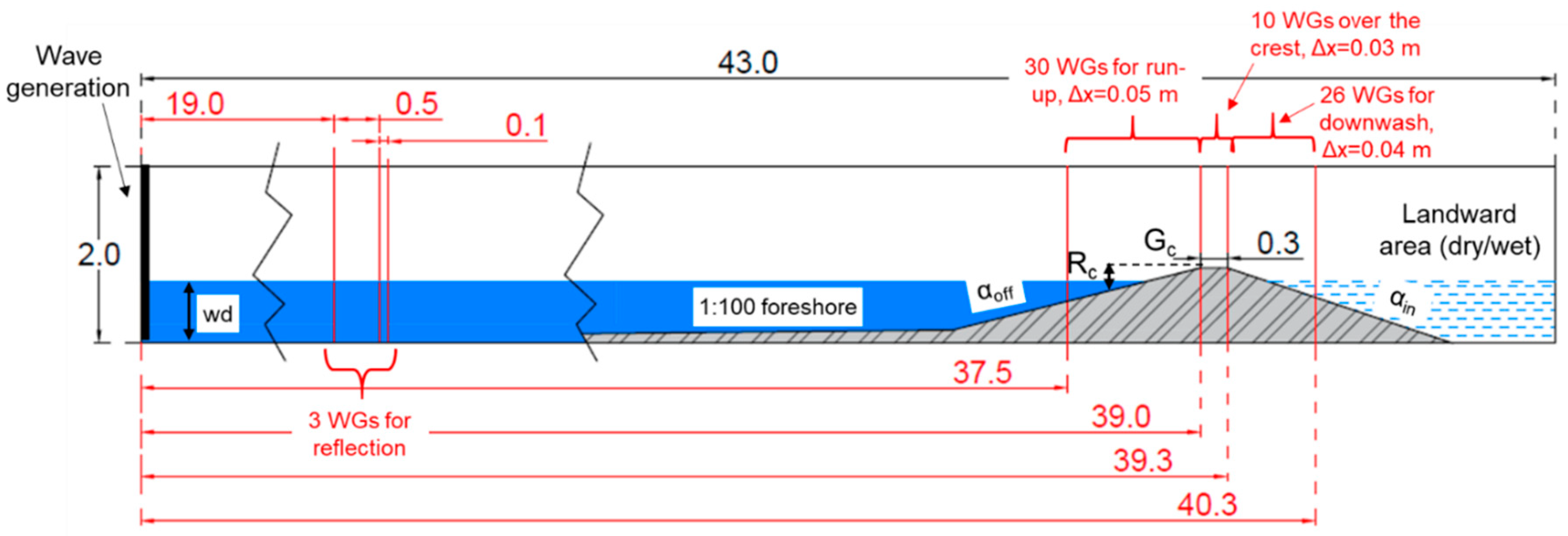
2.1. Numerical Setup and Tested Conditions

The numerical database employed in this contribution was collected by Formentin et al. (2014) [15] and updated by Formentin et al. (2018) [18]. It consists of 94 simulations of wave overtopping against smooth trapezoidal structures in a 2D numerical flume, 43 m long and 2.0 m deep. Irregular waves were generated in all the simulations, characterized by Jonswap spectrum, with a peak enhancement factor γ = 3.3. The variety of the tested conditions (reported in Table 1) included two significant wave heights Hs (0.1 or 0.2 m) and various peak periods Tp (ranging approximately from 1.3 to 6.5 s) specifically identified to test values of the wave steepness Hs/Lm−1,0 between 0.02 and 0.05, where Lm−1,0 is the wave length computed from the spectral wave period Tm−1,0.
Figure 1 displays the layout of the numerical flume, with reference to the adopted symbols. The structures consisted of smooth dikes with varying seaward slope (cot(αoff) = 4 or 6) and fixed landward slope (cot(αoff) = 3). The crest width (Gc) and the structure height (hc) were kept constant and respectively equal to 0.3 m and 0.85 m. The seven crest freeboard values (Rc), varying with the still water depth (wd), were selected to test positive, zero and negative freeboard conditions. The geometrical features and the wave characteristics were defined starting from the experiments on wave overtopping at dikes carried out in the small wave flume of the Leichtweiss Institute for Hydraulic Engineering of the Technical University of Braunschweig in Germany [4] and in the flume of WL|Delft Hydraulics in The Netherlands [5]. Those experiments represent, indeed, the basis of most of the literature studies aimed at characterizing the overtopping flow over the dike slopes and crest.
The structure off-shore edge was placed at a distance of 39 m from the numerical wave generator (see Figure 1). Following Van Gent [5], a 1:100 sloping foreshore was located in front of the structure to allow wave generation in deep water. A free outflow boundary condition was set at the right boundary of the numerical flume. The water depth landward the structure was either set to zero, “dry” conditions, or equal to the seaward water depth wd, “wet” conditions. The dry condition was used to represent the case of over-washed dikes or levees, while the wet condition represents the case of fully breached or submerged dikes. The first case (dry) represents, therefore, ordinary conditions in a climate change scenario, while the second one (wet) represents extreme, catastrophic conditions. The numerical modelling of the dry condition was achieved [18] modifying the right boundary condition of the original IH-2VOF numerical code [16], which was conceived to work with a constant water depth across the whole channel. The two different landward conditions, wet and dry, determine completely different processes of wave overtopping, and in turn, different values and evolution trends of the overtopping flow characteristics along the structure crest.
A constant mesh of Δz = 0.01 m was adopted to discretize the whole computational domain in the vertical direction (z, hereinafter), while a variable mesh was chosen for the cross-shore direction (x, hereinafter). The x-mesh was set up by keeping the it fine and constant Δx = 0.01 m in the area around the structure and by gradually increasing the grid size towards the right and the left boundary sections up to Δx ≈ 0.02 and 0.04 m, respectively.
For all the simulations, 69 wave gauges (wgs, hereinafter) were installed in the numerical flume to record the time-series of the free surface elevations h, the pressures p and the cross-shore directed flow velocities u in front of, over and behind the structure. In particular:
  • Three wgs were placed at approximately 19 m from the wave generator to estimate the wave reflection coefficient Kr based on the methodology by Zedlt and Skjelbreia [19];
  • Thirty and 26 wgs were placed, respectively, on the off-shore slope (between 37.5 and 39 m from the wave generator, interspaced with a uniform interval of Δx = 0.05 m) and on the in-shore slope (from 39.3 to 40.3 m, with Δx = 0.04 m); these gauges were installed for analyzing the wave run-up and the wave overtopping and calculating the wave transmission coefficient;
  • Eleven wgs (Δx = 0.03 m) were placed across the dike crest, from 39 to 39.3 m, to characterize the flow over the crest.

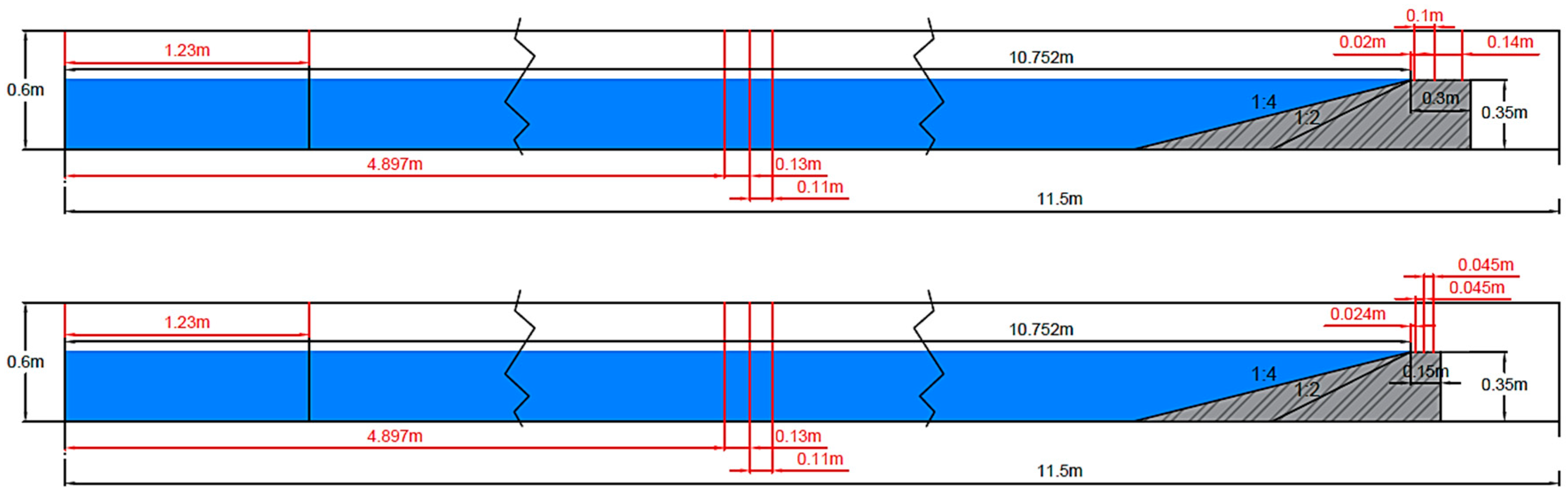
2.2. Experimental Setup and Tested Conditions

Sixty new experiments on wave overtopping at dikes were carried out in the wave flume of the Hydraulics Laboratory of the University of Bologna. The wave flume—displayed schematically in Figure 2a—is 12 m long, 0.5 m wide and 1.0 m deep and the waves are generated by the vertical movement of a cuneiform-shaped piston-type wave-maker under the control of the mass conservation law [20,21]. The maximum wave height and length are, respectively, Hs = 0.06 m and Lm−1,0 = 3 m, while the water depth wd before the wave-maker may be at maximum of about 0.4 m.
The setup of the lab experiments was based on the range of configurations and wave attacks tested with the numerical code, aiming at verifying and extending the numerical experience. Subject to the size of the wave flume of the laboratory and the constraints of the wave-maker, the experiments were conducted in 1:2 scale with respect to the numerical model scale. They consisted of irregular waves characterized by Jonswap spectrum with a peak enhancement factor γ = 3.3, wave heights Hs in the range 0.04–0.06 m and wave periods Tp ≈ 0.85–1.51 s, realizing values of Hs/Lm−1,0 ≈ 0.03–0.04. The wave attacks were performed against four dikes, whose cross-sections differed for the crest widths, Gc = 0.15 and 0.3 m, and/or the off-shore slope, cot(αoff) = 2 and 4. Figure 2b shows two out of the four dike configurations, where cot(αoff) = 2 is combined with Gc = 0.15 m (left) and cot(αoff) = 4 is combined with Gc = 0.30 m (right). The remaining two configurations (not shown for sake of brevity) were realized by combining cot(αoff) = 2 with Gc = 0.30 m and cot(αoff) = 4 with Gc = 0.15 m. All the structures were 0.35 m high (see Figure 2b) and were positioned in the wave-flume so that the spot of the dike’s off-shore crest edge was always at the same distance of 10.75 m from the wave-maker, as indicated in Figure 2a. Each dike configuration was tested with three crest-freeboard conditions, Rc/Hs = 0, 0.5 and 1, obtained by varying the water depth wd in the channel from 0.29 to 0.35 m. For each freeboard, several wave attacks were performed, by varying the values of Hs and Tp, resulting in a total of 60 tests. All the experiments were performed in dry landward conditions.
A specific label (ID) was defined to identify each test performed. This ID consists of 12 alphanumeric symbols forming five groups of chars, e.g., “R00-H04-s4-G15-c2,” where:
  • The 1st group includes three symbols, which may be “R00,” “R05” or “R10,” and refers to the target value of Rc/Hs (R00 stands for Rc/Hs = 0; R05 stands for Rc/Hs = 0.5 and R10 stands for Rc/Hs = 1.0);
  • The 2nd group may be “H04,” “H05” or “H06” and each represents the target Hs value (respectively 0.04, 0.05 and 0.06 m);
  • The 3rd group includes “s3” or “s4” and refers to the target wave steepness sm-1,0 = Hs/Lm-1,0 = 0.03 or 0.04;
  • The 4th group is “G15” or “G30,” which refer respectively to Gc = 0.15 or 0.3 m;
  • The 5th group is “c2” or “c4” and refers to cot(αoff) = 2 or 4, respectively.
The summary of the tested configurations in the laboratory is given in Table 2.
As shown in Figure 2a, the wave-flume was equipped with the following instruments:
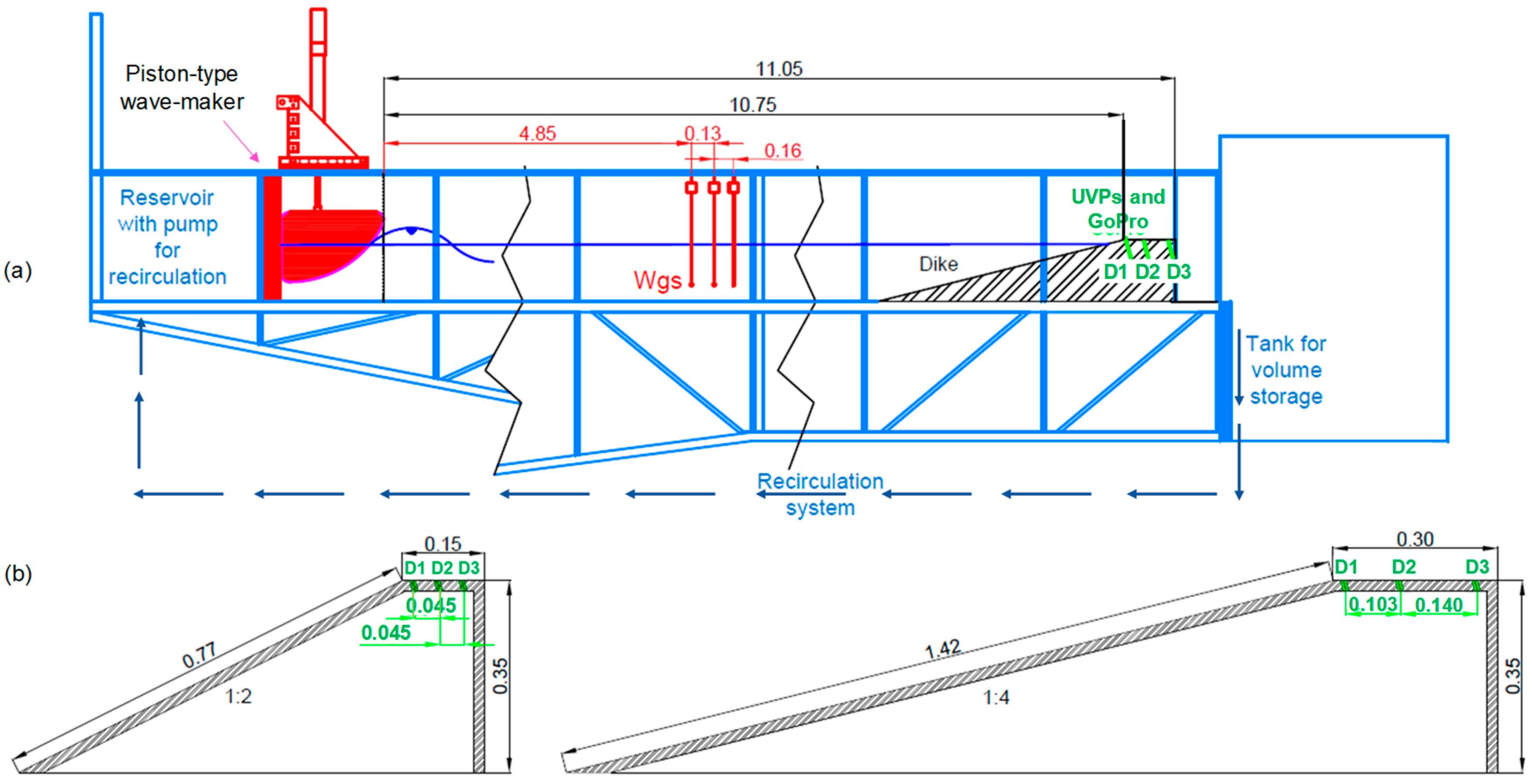
  • Three wgs, placed at approximately 1.5 times the maximum Lm−1,0 from the wave-maker (≈5 m) to record the free-surface elevation with a sampling frequency of 100 Hz and separate the incident and reflected waves; the positions of the wgs are displayed in Figure 2a in red color.
  • Three ultrasonic Doppler velocity profilers (UVPs), which were installed along the structure crest and were used to record the time series of the vertical profiles of the horizontal flow velocities u and track the free surface elevation h. The positions of the three UVPs, shown in Figure 2b in green color and referenced as D1, D2 and D3, were selected to reconstruct the statistics of h and u in proximity of the dike crest off-shore edge (D1), in the middle of the crest (D2) and close to the in-shore edge (D3).
  • A tank for the storage and the measurement of the overtopping volumes, placed at the end of the wave flume and below the channel and connected to recirculation system, regulated by a flowmeter (precision q = 1 × 10⁻⁵ m3/s), which collects the overtopped water from the tank and brings it back to the reservoir placed upstream the channel.
  • A 30 Hz full-HD camera to film the wave run-up and overtopping process; the camera was installed in front of the channel and corresponding to the upper part of the dike slope and the dike crest.
  • All the structures were realized in a very smooth plexiglas material, which can be characterized by a roughness factor of γf = 1 [13].

2.3. Methodology for the Reconstruction of the Overtopping Flow Characteristics

For the numerical tests, the instantaneous values of h and u were directly derived from the time series recorded at the 10 numerical wgs placed along the structure crest (see Figure 1), while for the laboratory experiments, they were derived from the three UVPs measurements of the particle velocities and echoes. The monostatic sonar emits and receives short bursts composed by acoustic pulses to measure profiles of flow velocity at the probe location [22] by exploiting the Doppler effect. The following procedure was adopted.
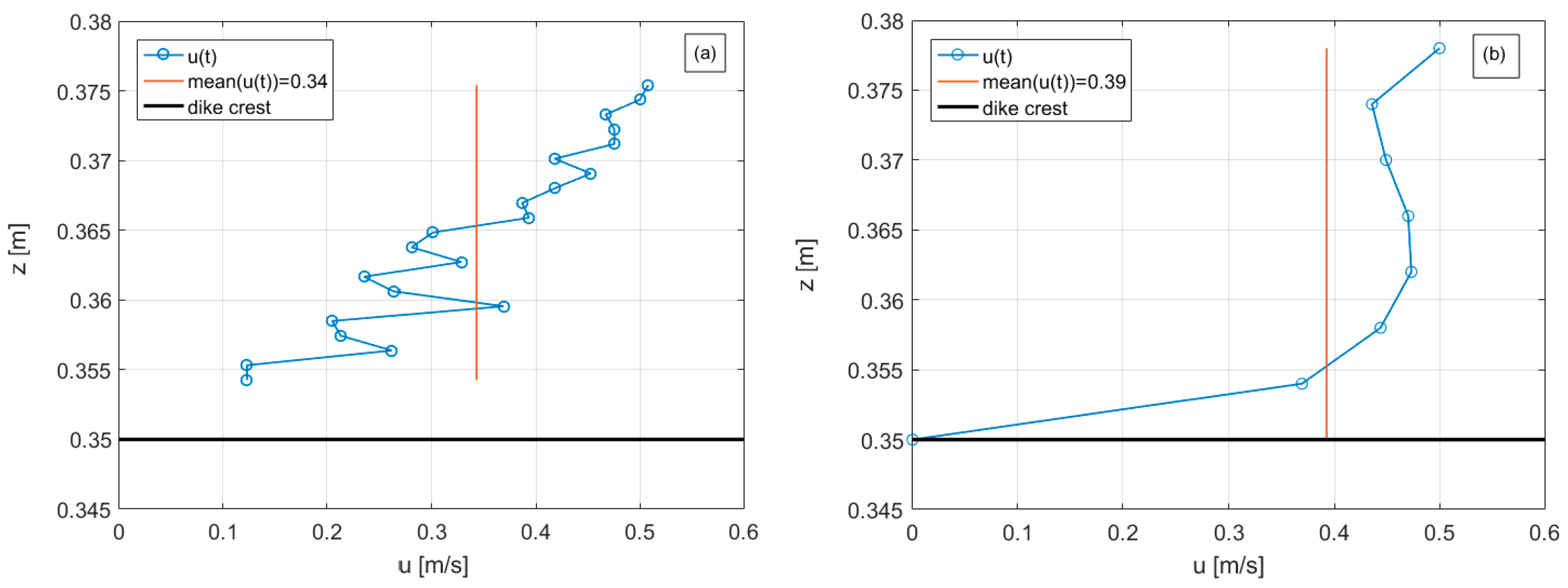
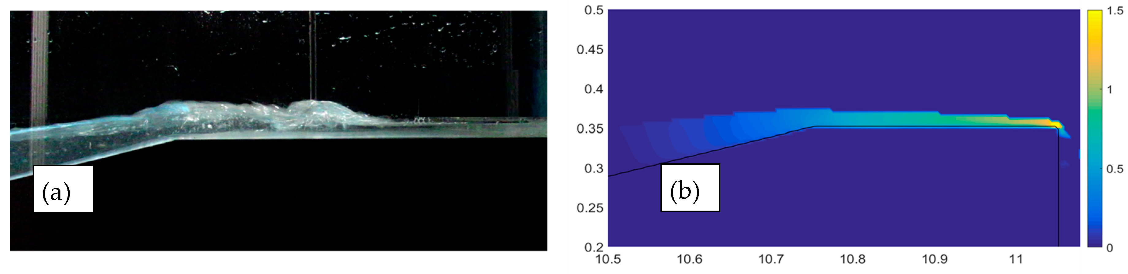
  • u. At each time step, the UVPs recorded a vertical profile of the radial velocity along the acoustic beam that was forming a 15°-angle (i.e., the Doppler angle) with the horizontal crest of the dike. The actual velocity was then reconstructed by assuming horizontal vectors (i.e., aligned flow with the dike crest). The range of the measured velocities depended on the settings of the probes; i.e., emitting frequency, pulse repetition period, the beam width and the Doppler angle. In the present experiments, the UVP settings yielded ~10 cm as the maximum layer thickness (as expected to occur above the dike crest during the largest wave attacks with Hs = 0.06 m), with a profile resolution of 1.01 mm, and 4.2 m/s as the maximum velocity, with a nominal accuracy of 0.1% depending on the developing turbulence patterns in the test.
  • h. At each time step and with the same spatial resolution of the flow velocities, the UVPs also recorded the vertical profiles of echo (dB) of the acoustic impulse reflected by the particles transported by the water. In accordance with the free surface, the acoustic impulse undergoes a strong reflection induced by the density variation, which determines, in turns, a sharp peak of the echo value. The time series of the free surface elevations, and of the layer thicknesses h, were reconstructed based on the peak position in the instantaneous vertical profiles of the echo.
For both the numerical simulations and the laboratory experiments, the instantaneous depth-averaged values of u were calculated from the vertical profiles. The time series of h and u were treated as stochastic variables, calculating the following statistics: mean, standard deviation, median, minimum, maximum and upper 2% percentiles (namely, h2% and u2%). Based on the literature [5], these latter quantities were, respectively, the values of h and u exceeded by 2% of the incoming waves and were used by several authors [1,4,5,8] to characterize the extreme overtopping flow.
The records of the tests obtained with the camera were also elaborated to derive the envelopes of the free-surface elevations through the implementation of ad hoc image processing algorithms. In this study, a few results of the envelopes are presented as a validation of the numerical code. More details about this technique and the results obtained are given in reference [23].

2.4. Scale and Model Effects

Neither the experimental nor the numerical tests refer to real prototype structures, but the setup of the hydraulic and structural parameters aimed at represent “realistic” conditions. In particular, the whole numerical and experimental campaign was inspired to the experiments on dikes carried out in 1:10 scale by Schüttrumpf and Oumeraci [7]. Since the same structural dimensions and the same wave conditions tested by Schüttrumpf and Oumeraci were adopted for the numerical modelling, it can be assumed that the numerical tests were conducted at 1:10 scale by the Froude similarity law. Since the experiments were conducted in 1:2 scale with respect to the numerical modelling, a scale factor of 1:20 can be considered for the laboratory tests.
The adoption of the Froude similarity law necessarily involves the distortion of the ratios of other forces, such as inertia to surface tension (Weber number) and inertia to viscosity (Reynolds number).
An incorrect scaling of the surface tension can affect the dynamics and the type of the wave breaking [24]. Specifically, the surface tension increases with decreasing length scale, and for shorter waves (wave lengths L < 4 m) the increased surface tension tends to inhibit the wave plunging [24]. A plunging breaker type at prototype scale might, thus, transform into a spilling breaker at model scale, with a reduction of the wave energy dissipation. Despite all the experimental tests present values of L < 4 m (0.9 < L < 3.30 m), the occurrence of fully-plunging was systematically observed and filmed, and, globally, no relevant effect of a reduced wave energy dissipation was observed (see Section 3).
A distorted representation of the fluid viscosity leads to lower Reynolds numbers and larger viscous forces [25,26,27] in the model tests. Indeed, the experiments were characterized by Reynolds numbers in the range 7 × 10³–5 × 10⁴, which, rescaled to prototype conditions, correspond to Reynolds numbers in the range 5 × 10⁵–2 × 10⁶. Overall, reduced Reynolds numbers might determine higher drag coefficients, and consequently, smaller run-up heights and less overtopping at small scale [26]. However, the effects of increased drag forces on the overtopping due to scale effects are considered to be relevant for rubble mound structures, while they tend to be less effective or negligible for smooth structures [28,29].
The results of the experimental tests confirm that, on average, the effects of the surface tension and of the viscosity on the overtopping are modest or negligible: the average values of q are indeed in line with the predictions by literature methods (see Section 3.1), and no systematic overestimation or underestimation was observed. This analysis cannot assure, though, that viscosity and surface tension may not induce local and/or instantaneous effects, which are not quantifiable with the available instrumentation.
The small scale adopted for the experiments may also result in a smaller amount of air bubbles entrapped in the overtopping flow [30]. The reduced presence of air bubbles (with respect to larger scales or prototype conditions) is expected to induce smaller wave energy dissipation, and overall, higher run-up, higher overtopping rates and higher values of the overtopping flow characteristic. Though the effective rate of the air entrainment has not been quantified yet, the presence of air bubbles was systematically observed during all the experiments. Research is ongoing to get precise estimations based on the analysis of the videos and the image processing.
The experimental tests might be also affected by “side effects,” due to the relatively small width of the wave flume (50 cm). These side effects might determine distortions or asymmetries of the wave shape in the longshore direction, which were not measured but were not visually observed. To limit the influence of these effects, all the measurements (free surface elevations, flow depths, flow velocities) were taken in the middle section of channel.

3. Verification of the Data

This Section is dedicated to the characterization and verification of the new experimental and numerical data and to the model validation. The data are compared to existing prediction methods in terms of q and Kr in Section 3.1 and Section 3.2, respectively. For q, the EurOtop equations [28] and the artificial neural network (ANN) developed by the authors [31,32,33] were considered. The data of Kr were instead compared to the formula by Zanuttigh and van der Meer [34] and to the ANN.

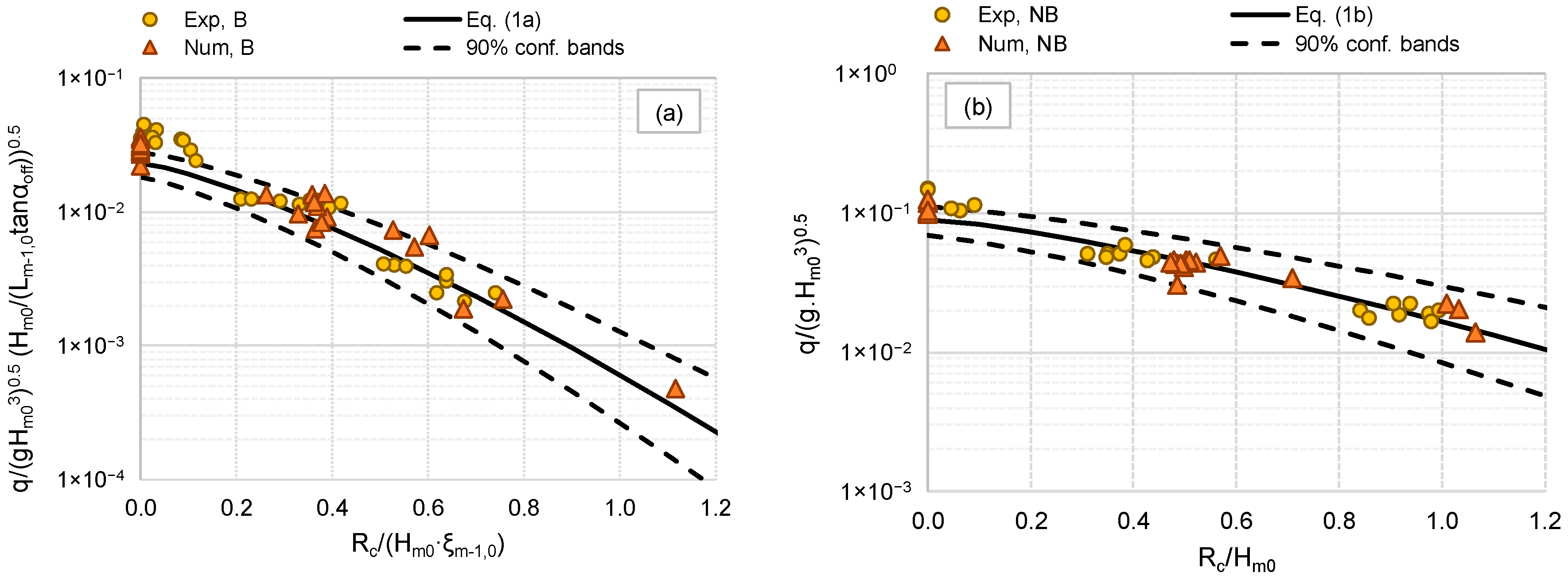
3.1. Wave Overtopping Discharge

The most commonly-adopted method for the prediction of q in case of Rc/Hs ≥ 0 and dry landward conditions is represented by the formulae of EurOtop (2018). For a probabilistic design and following the mean value approach, these formulae give:
q g H m 0 3 = { ( 1 a ) 0.023 t a n α o f f · γ b · ξ m - 1 , 0 · e x p ( - ( 2.7 · R c ξ m - 1 , 0 · H m 0 · γ b · γ f · γ v · γ β ) 1.3 ) ( 1 b ) with   a   maximum   of   0.09 · e x p ( - ( 1.5 · R c H m 0 · γ f · γ β ) 1.3 )
where ξm−1,0 is the Iribarren–Battjes breaker parameter and the factors γb, γf, γv and γb are the reducing coefficients for a berm, the roughness of the armor layer, the presence of a crown wall and oblique wave attacks. In the new numerical and experimental tests presented in this paper, all these factors are equal to 1. The two formulae Equations (1a) and (1b) are respectively valid for breaking (i.e., approximately for values of ξm−1,0 ≤ 2) and non-breaking (ξm−1,0 > 2) wave conditions, where the wave breaking is supposed to occur for the interaction between the wave and the structure slope (αoff).
The new data of q are compared to the curves representing Equations (1a) and (1b) in Figure 3a,b, respectively. In both charts, the data are distinguished by numerical (triangles) and experimental (circles) tests and are plotted against the relative freeboard. The values of Rc/Hs were computed from the incident wave heights Hs, measured at the structural toe instead of the target values reported in Table 1 and Table 2. In both charts, only the tests at Rc/Hs ≥ 0 and dry landward conditions are plotted. On average, the data are straightly and symmetrically distributed around the [28] curves. Most of the data fall within the 90% confidence bands associated to the predicting formulae (dashed lines in Figure 3). The greatest scatter is observed around the zero freeboard, where the formulae seem to underestimate part of the numerical and experimental data. Quantitatively, the agreement among the data and Equations (1a) and (1b) is provided for both the numerical and the experimental data in Table 3 in terms of the error indexes R2 (coefficient of determination) and of σ% (relative standard deviation or coefficient of variation). Numerical data are significantly better predicted by Equations (1a) and (1b) than the experimental data, being σ% = 16% and R2 = 0.95 in case of the numerical dataset and σ% = 56% and R2 = 0.87 in case of the laboratory dataset. The lower agreement found for the experimental data is principally caused by the underestimation bias at Rc/Hs = 0, as it can be appreciated by Figure 3.
The data were further checked against the predictions of q obtained with the ANN predicting tool [30,32,33]. Differently from the EurOtop equations, the ANN can be applied to structures at negative freeboard as well, but still in dry landward conditions exclusively. The comparison among experimental/numerical values of q and the corresponding ANN predictions is given in Figure 4, while the error indexes σ% and R2 are reported in Table 3. The agreement between the predictions and the measurements is remarkable in case of the laboratory dataset (σ% = 12% and R2 = 0.91), as all the data are concentrated around the bisector line in Figure 4. The slight underestimation bias (μ(qANN/qlab) = 0.89) could be explained with the particular smoothness of the dike material (plexiglas), which has been quantified with γf = 1, whereas in the ANN training database the value of γf = 1 is generally associated to concrete, asphalt, plywood, grass, etc. The values of q associated to the numerical dataset (σ% = 27% and R2 = 0.81) are more scattered but still fairly represented by the ANN, as almost all the data fall within the 90% confidence bands (dashed lines in Figure 4) and no significant bias is observable.
The analysis of the data at negative freeboard and wet landward conditions is provided in [18], where a specific method for the prediction of q in such conditions is presented. As this method is the only available in the literature so far, the data are not reported here again, as they cannot be used for validation. Anyway, the main focus of this paper is on dry landward conditions. The dry landward conditions represent, indeed, the ordinary conditions, while the wet landward conditions represent the case of fully breached dikes; i.e., extreme conditions.

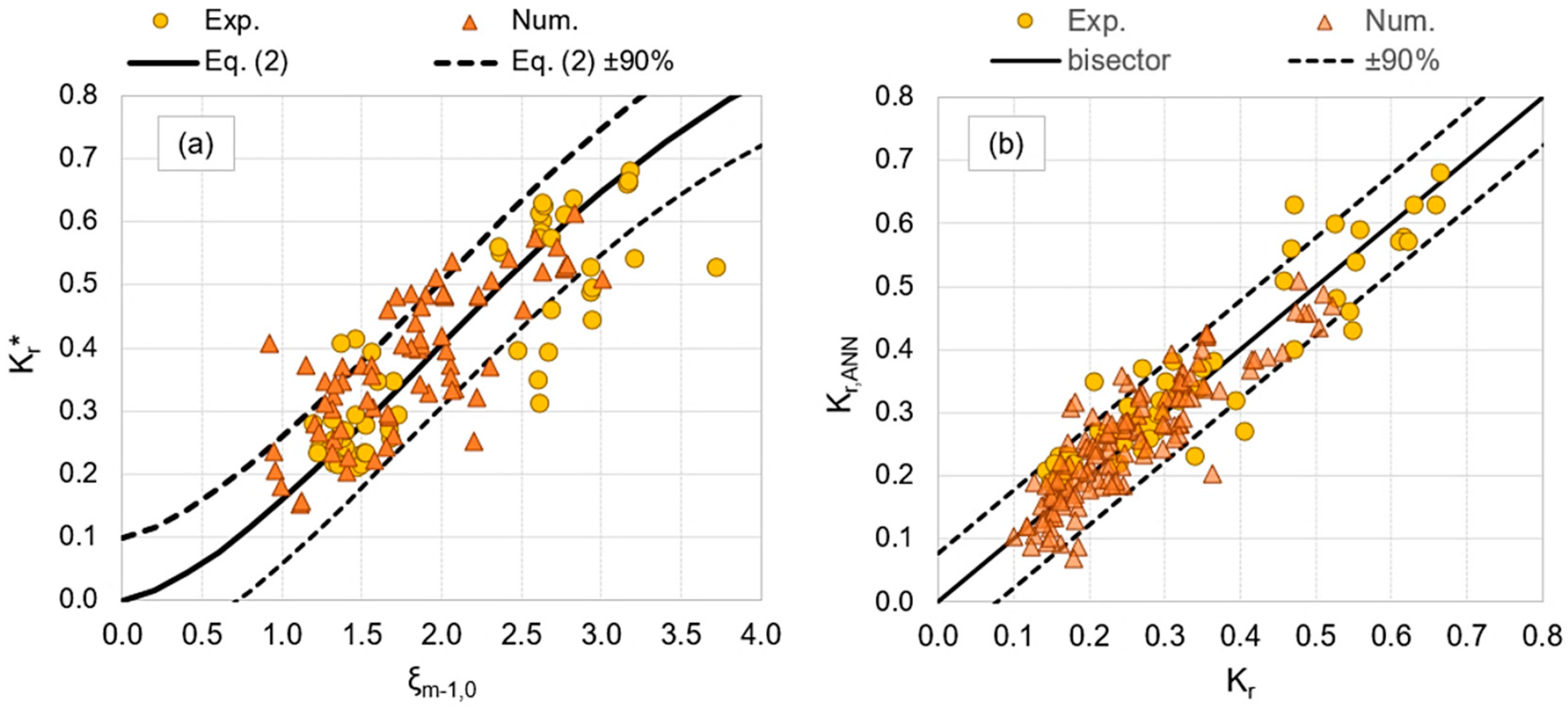
3.2. Wave Reflection Coefficient

The data of Kr resulting from the numerical simulations and the laboratory tests were compared to the predicting formula by Zanuttigh and van der Meer [34], which gave:
K r = tan h ( a × ξ m - 1 , 0 b ) · { 1 , if   R c H s 0.5 0.67 + 0.37 × R c H s , if   - 1 R c H s < 0.5
where a = 0.16 and b = 1.43 when γf = 1. Equation (2) is valid for values of the wave steepness sm−1,0h ≥ 0.01.
The qualitative comparison among the new data of Kr and the curve representing Equation (2) is provided in Figure 5a. In this chart, the quantity Kr* is shown as a function of ξm-1,0, where Kr* = Kr if Rc/Hs ≥ 0.5, and Kr* = Kr/(0.67 + 0.37∙Rc/Hs) if −1 ≤ Rc/Hs < 0.5. All the data beyond the range of validity of Equation (2) have been removed from the plot.
Figure 5a shows that almost all the numerical tests (triangles) are included within the 90% confidence bands (dashed lines), while a slightly higher scatter was observed for the laboratory tests (circles), especially when ξm−1,0 > 2.5. The presence of a few “outliers,” i.e., data that fall outside the 90% confidence bands, can be explained by considering that Equation (2) represents an average trend and was fitted mostly on rubble mound data. Quantitatively, the agreement among the data and the formula is represented by σ% = 45% and R2 = 0.77 in case of the laboratory tests and σ% = 28% and R2 = 0.90 in case of the numerical tests, as reported in Table 3. These error indexes are in line with the uncertainty associated to Equation (2) (see [34]).
The comparison with the predictions of Kr obtained with the ANN [33] is qualitatively given in Figure 5b and quantitatively characterized by the error indexes of Table 3. All the numerical and experimental tests fall within the range of applicability of the ANN. Both Figure 5b and Table 3 indicate that the data are slightly better represented by the ANN than Equation (2), with σ% = 40% and 6.0% and R2 = 0.89 and 0.93 for the laboratory and numerical datasets, respectively. This can be explained with the higher number of parameters involved in the ANN with respect to the formula.

4. Validation of the Numerical Code

The numerical code was validated against a dataset of 12 tests selected among the 60 new experiments carried out in the wave flume (see Section 2.2). The 12 tests were reproduced with the modified IH-2VOF code and the resulting values of the average wave overtopping discharge q, of the wave reflection coefficient Kr (Section 4.1) and of the flow depth h and velocities u at the dike crest (Section 4.2 and Section 4.3) were compared to the corresponding laboratory measurements.
A specific numerical channel and an ad hoc mesh grid were set up to exactly reproduce the wave flume and the position of the wgs in the lab. The mesh resolution Δz was set constant across the numerical channel and equal to 0.004 m, while the horizontal mesh was made variable by keeping the finest grid of Δx = 0.004 m in the area around the structures. Six numerical wgs were set in accordance with the laboratory instruments; i.e., three of the resistive gauges for the separation of the incident and reflected wave heights (at around 5 m from the wave-maker) and three of the UVPs along the dike crests. The layout of the numerical channel and the displacement of the numerical gauges are shown in Figure 6. The reproduced dike configurations with G30 and G15 are respectively reported at the top and at the bottom of Figure 6.
The 12 selected tests, whose characteristics are reported in Table 4, cover the variety of the geometrical configurations tested in the laboratory, precisely: two dike slopes, c2 and c4; three relative crest freeboards R00, R05 and R10; and two crest widths, G15 and G30. The simulated wave conditions were the same for all the 12 tests and refer to the target wave height H05 and the target wave steepness s3. Each simulation was made lasting 480 s (like in the lab) and a sampling frequency of 20 Hz was adopted for recording the values of h and u at the numerical wave gauges.

4.1. Wave Overtopping and Wave Reflection

For each test, Table 4 reports the values of the hydraulic parameters (Hm0, Tm−1,0 and ξm−1,0) measured in the laboratory (column “Lab”) and derived from the numerical model (column “Num”), including the dimensionless average values of q, q/(gHm0Tm−1,0) and the values of Kr. For each parameter, the mean μ and the standard deviation σ representative of the distribution of the ratio between numerical and experimental values (num/lab) are provided. Overall, the values of μ(num/lab) related to Hm0, Tm−1,0 and ξm−1,0, which are respectively equal to 0.87, 1.02 and 1.11, suggest that the code well reproduces the target wave conditions. The agreement between numerical and laboratory wave periods is remarkable (μ = 1.02, with σ = 8.4%), while the wave heights were slightly underestimated in the numerical code (μ = 0.87, σ = 8.0%). This result is line with the tendency of the IH-2VOF code to reduce the wave steepness by generating lower wave heights with respect to the target values, especially when the waves are generated in intermediate depth water (see, all of [15,16]), as in the present case. The lower values of sm−1,0 obtained with the numerical code determined, in turn, slightly higher values of ξm−1,0 (μ = 1.11, σ = 9.75%); i.e., wave conditions slightly more distant from the wave breaking.
As for q and Kr, the values of μ respectively equal to 0.94 and 0.96 indicate that on average the code can very well represent both the overtopping and the reflection processes, giving a very modest underestimation of both the quantities (μ < 1). The underestimations can be explained considering the different methodologies adopted in the numerical code and in the laboratory to calculate q and the different sampling frequencies used to record the free-surface elevations at the three wgs to reconstruct Kr (100 Hz in the lab and 20 Hz in the numerical code). The lab values of q correspond to the average quantities measured from the tank (see Section 2.2), while the numerical values were derived from the integration of the values of u by the corresponding values of h recorded at the dike off-shore edge. Nevertheless, the differences between numerical and experimental values are on average 5%, with standard deviations of 16% (Kr) and 28% (q), which are very limited and significantly lower than the average uncertainty associated to the common predicting methods (see, e.g., [34] or [35] for Kr, and [28] for q).

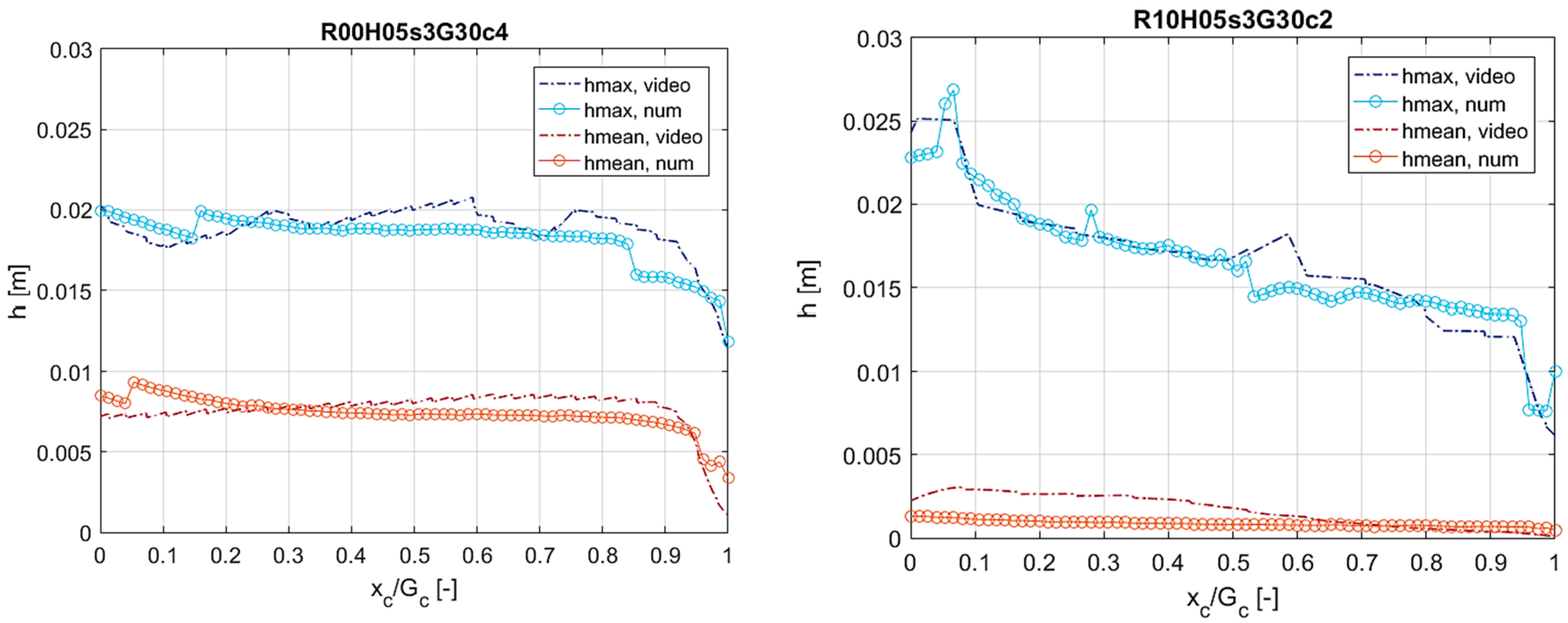
4.2. Water Depth Envelopes

The validation of the flow depths is given by comparing the maximum and mean envelopes of the h-values obtained with the numerical code to the corresponding envelopes derived from the image processing of the video of the tests recorded with the camera installed in the laboratory. The reconstruction of the free surface elevation from the image processing was based on automatic algorithms of pattern recognition, which were implemented after the phases of calibration of the camera, background removal and the application of filters to remove the noise from the signals. The details about the procedure and the algorithms applied to reconstruct the free surface elevation from the videos are given in [23].
The comparison among the envelopes is qualitatively given in Figure 7 for two tests (R00H05s3G30c4 and R10H05s3G30c2) selected from the dataset of validation (see Table 4) and presenting different crest freeboards (R00 and R10) and slopes (c4 and c2). In both cases, the numerical envelopes follow the trends from the videography, showing the same decrease rates and very similar values of the maximum and mean h at the extremes of the dike crest. To assess the level of agreement between the corresponding envelopes, the maximum reciprocal distances can be considered: ~2 mm for the maximum envelopes of both the tests, and respectively ~0.5 mm and ~1 mm for the mean envelopes of test R00H05s3G30c4 and test R10H05s3G30c2. These tests are representative of the whole dataset, and the same accuracy was achieved for all the 12 tests.

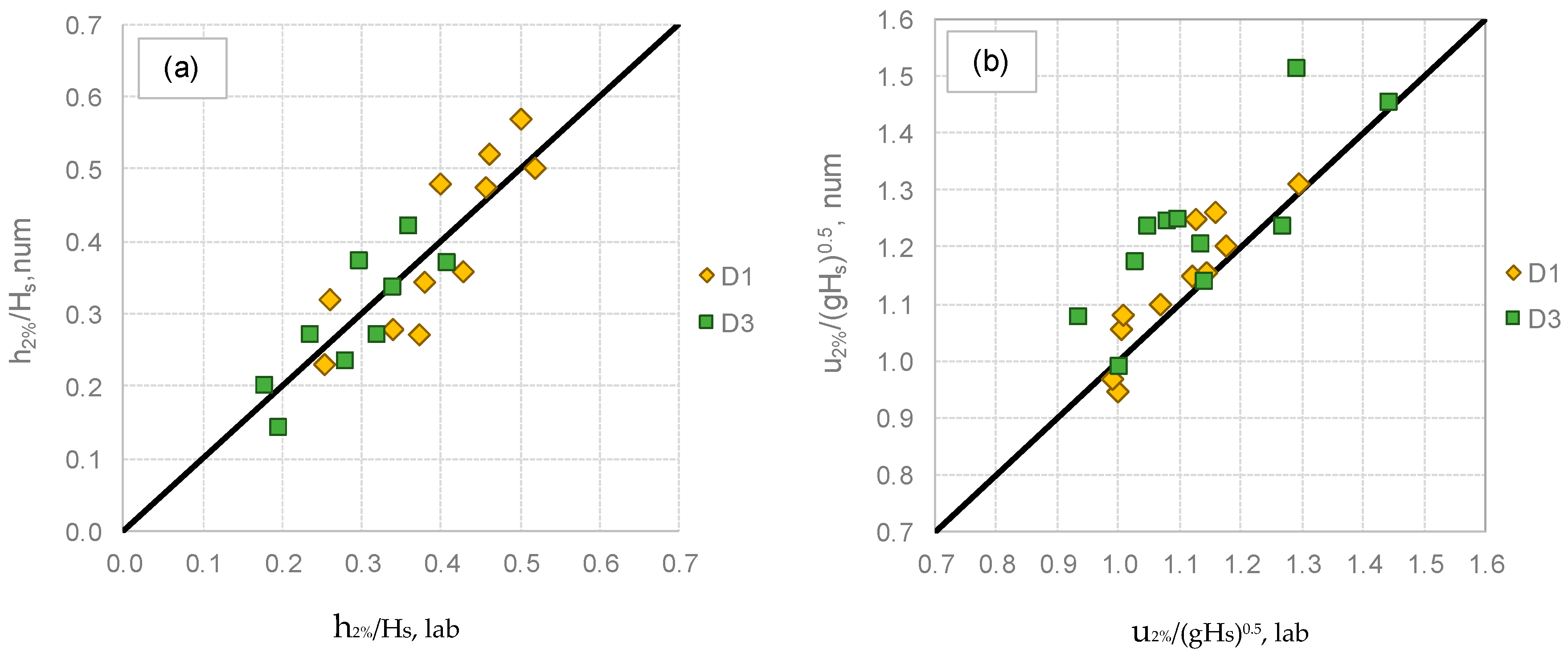
4.3. Extreme Flow Depths and Velocities

The numerical values of h2% and u2% calculated at the edges of the dike crest (precisely, at D1 and D3, see Figure 2b) are compared here to the corresponding values extracted from the elaboration of the echo and velocity profiles recorded from the UVPs installed at the same positions on the dikes in the laboratory. This analysis proposes a punctual verification of the numerical data, as it is not possible to draw the envelopes of the h and u-values from the UVPs measurements, which are available in accordance with the three UVPs only.
The comparison is qualitatively shown for all the tests of the dataset of validation (Table 4) in Figure 8. The data of h and u are made dimensionless through the terms Hs and (gHs)0.5, respectively, to account for the different wave conditions generated in the numerical and laboratory flumes. The numerical values of h2% (Figure 8a) at both D1 and D3 are symmetrically distributed around the bisector line, representing the perfect association with the corresponding laboratory data. The agreement is represented by values of the standard deviation σ respectively equal to 0.006 m and 0.005 m for D1 and D3; the corresponding relative standard deviations (or coefficient sof variation) σ% are 26% and 30%.
Most of the numerical values of u2% in Figure 8b are aligned directly with or above the bisector line, suggesting that, on average, the numerical code gives slightly overestimations of u2%. This tendency is observed at both D1 and D3 and can be quantified with a value of μ(u2%,num/u2%,lab) = 1.03 and 1.09 for D1 and D3, respectively. Overall, the standard deviation associated to the two distributions is σ = 0.09 m/s and 0.12 m/s at D1 and D3, respectively, with σ% = 9.8% at D1 and 13.7% at D3. The slight tendency to overestimate the u-values by the numerical code is probably due to the different representation of the friction with the dike surface and of the air entrainment. The IH2VOF code, indeed, is monophasic and cannot account for the air bubbles entrapped in the overtopping flow within the experiments (see Section 2.4). The air entrainment might induce a larger wave energy dissipation in the laboratory tests with respect to the numerical modelling and reduce, in turn, the experimental flow velocities.

5. Extreme Flow Depths and Velocities at the Dike’s Off-Shore Edge

This Section proposes a systematic and detailed analysis of the overtopping flow characteristics at the off-shore edge of the dike crest. In Section 5.1, the extreme percentiles of h2% and u2% resulting from the numerical and experimental modelling are compared to the literature formulae. After discussing the performance of the existing methods and investigating the reasons of the discrepancies between data and formulae (Section 5.2), a new fitting is proposed to update the state-of-the-art formulae for the prediction of h2% and u2% at the off-shore edge.

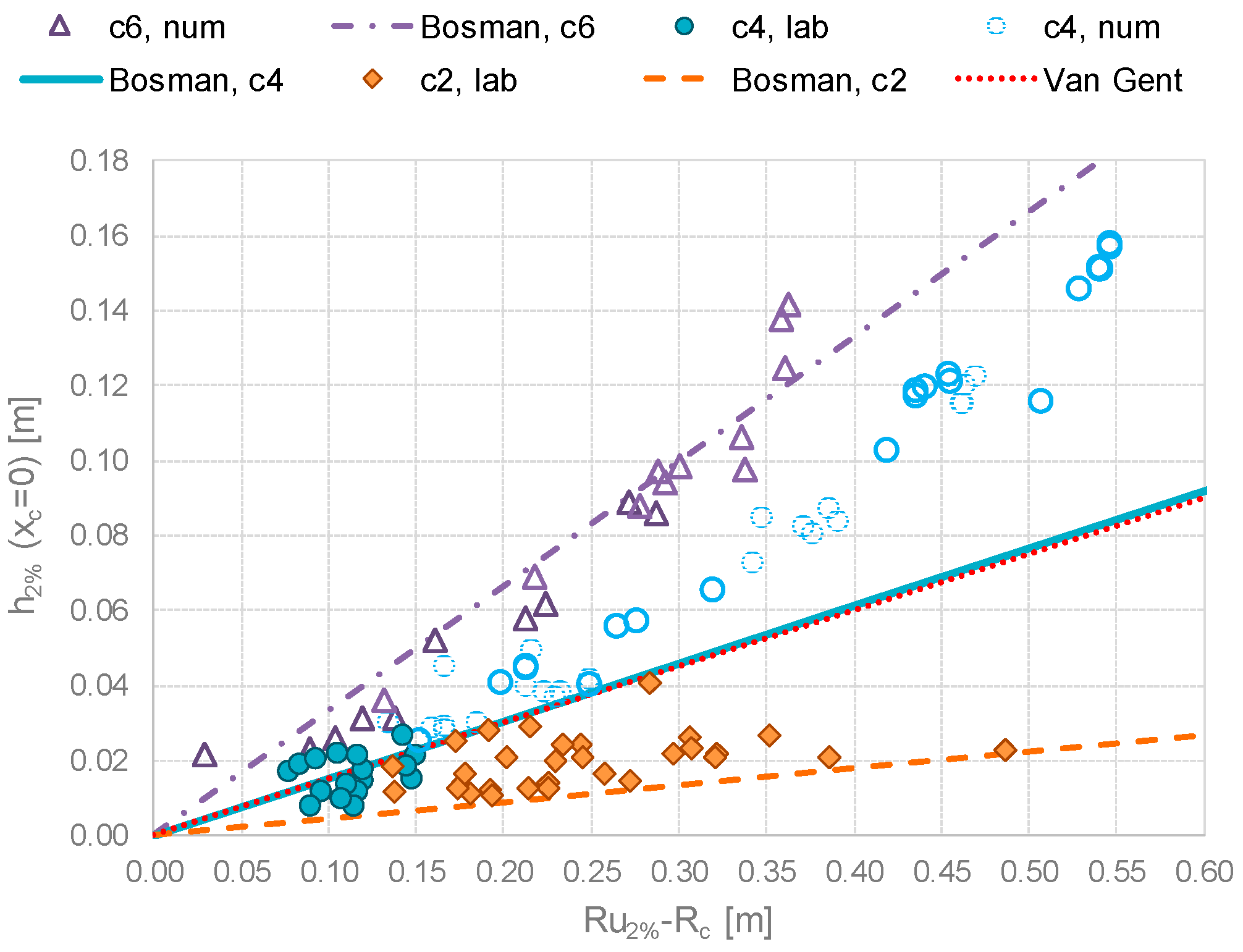
5.1. Comparison with Literature Formulae

All the formulae available in the literature for the evaluation of h and u at the extremes of the structure crest [1,5,7,8] draw on the following overarching scheme originally [4]:
h2%(xc = 0) = ch × (Ru,2%RC), RC ≥ 0
u2%(xc = 0) = cu × [(Ru,2%RC)]0.5, RC ≥ 0
where the values h2% and u2% are, respectively, the flow thicknesses and the flow velocities at the off-shore edge (xc = 0) of the dike crest that are exceeded by the 2% of the incident waves. The estimations of h2% and u2% by Equations (3) and (4) depend on Ru,2%, which is the value of the wave run-up exceeded by the 2% of the waves and can be calculated based on EurOtop [28]. The values or the formulations proposed by the various authors for the coefficients ch and cu are summarized in Table 5. In the earliest formulae [4,5], the fitting coefficients ch and cu are constant values, while in more recent methods [1,8], ch and cu are functions of the off-shore slope αoff. Moreover, while the formulations for u2% by Schüttrumpf [4] and Van Gent [5] were targeted to represent the flow velocities, the formulations by Bosman et al. [8] and by van der Meer et al. [1] aim at predicting the front velocities, or wave celerities, giving higher estimations of u2%.
Figure 9 and Figure 10 compare, respectively, the values of h2%(xc = 0) and u2%(xc = 0) gathered with the new numerical and experimental modelling to the corresponding predicting formulae; i.e., Equations (3) and (4). In both Figure 9 and Figure 10, the results are grouped by values of cot(αoff) and refer to tests in dry landward conditions Rc/Hs ≥ 0. The data are further distinguished between experimental (filled-in symbols) and numerical (void symbols). The two charts of Figure 10 show the tests at Rc/Hs > 0 (panel a) and Rc/Hs = 0 (panel b). Following the structure of Equations (3) and (4), the results are shown as functions of (Ru,2%Rc) in Figure 9 and of (g∙(Ru,2%Rc))0.5 in Figure 10.
To ease the comparison, only the formulations by Van Gent [5] and Bosman et al. [8] are shown. The curves representing the formulae by Schüttrumpf [4] are very close to the curves by Van Gent, while the curves by van der Meer et al. [1] for u2% (Figure 10) are close to the curves by Bosman et al. [8]. It should be noted that Bosman et al. [8] provided fittings for cot(αoff) = 4 and 6, exclusively (see Table 5). The curves for the prediction of h2% and u2% in case of cot(αoff) = 2 have been extrapolated from the original formulae by Bosman et al. [8]. For brevity, the notations “c2,” “c4” and “c6” will be used in the following to refer to cot(αoff) = 2, 4 and 6, respectively (see Section 2.2).
The analysis of Figure 9 suggests that:
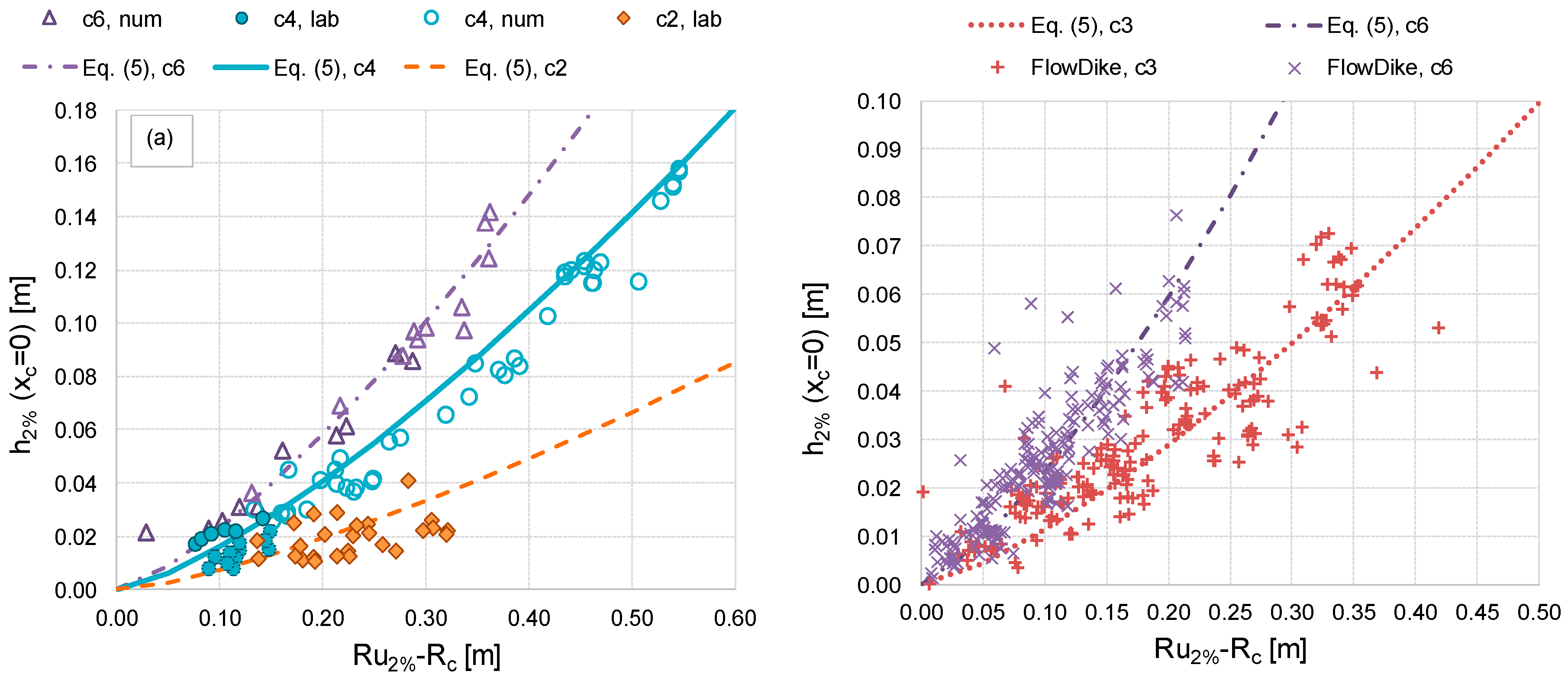
  • All the values of h2% fall within the straight lines representing the theoretical formulae, with the exception of one test at c6 that slightly exceeds the upper line by Bosman et al. [8] for c6 (dot-dashed line).
  • In agreement with Bosman et al., all the data show a non-negligible effect of the structure slope: the milder the slope, the higher h2%.
  • The formulation by Van Gent [5]—which does not account for the slope effect—can be used to get an “average” estimation of the values of h2%.
  • For modest values of the wave run-up, i.e., for (Ru,2%Rc) < 0.10–0.15, the formulae by Bosman et al. (2008), give an accurate representation of the data, while for (Ru,2%Rc) > 0.15, the formulae underestimate the values of h2% in case of c2 and c4. The underestimation increases when increasing (Ru,2%Rc), and reaches ~100% when (Ru,2%Rc) ≈ 0.45 (data c4, circles in Figure 7). This might be in part explained by considering that the experimental tests used to calibrate the formulae were characterized by values of (Ru,2%Rc) ranging between 0 and 0.3.
  • Overall, the data seem to follow a non-linear trend with (Ru,2% − Rc) and a refitting of Equation (3) to extend its validity to the cases of c2 and (Ru,2%Rc) > 0.3 will be discussed in Section 4.2.
A separate analysis was performed to investigate further potential effects of Rc/Hs and sm-1,0 on h2%, without leading to any relevant result.
As for the values of u2%(xc = 0), the analysis of Figure 10 leads to the following considerations.
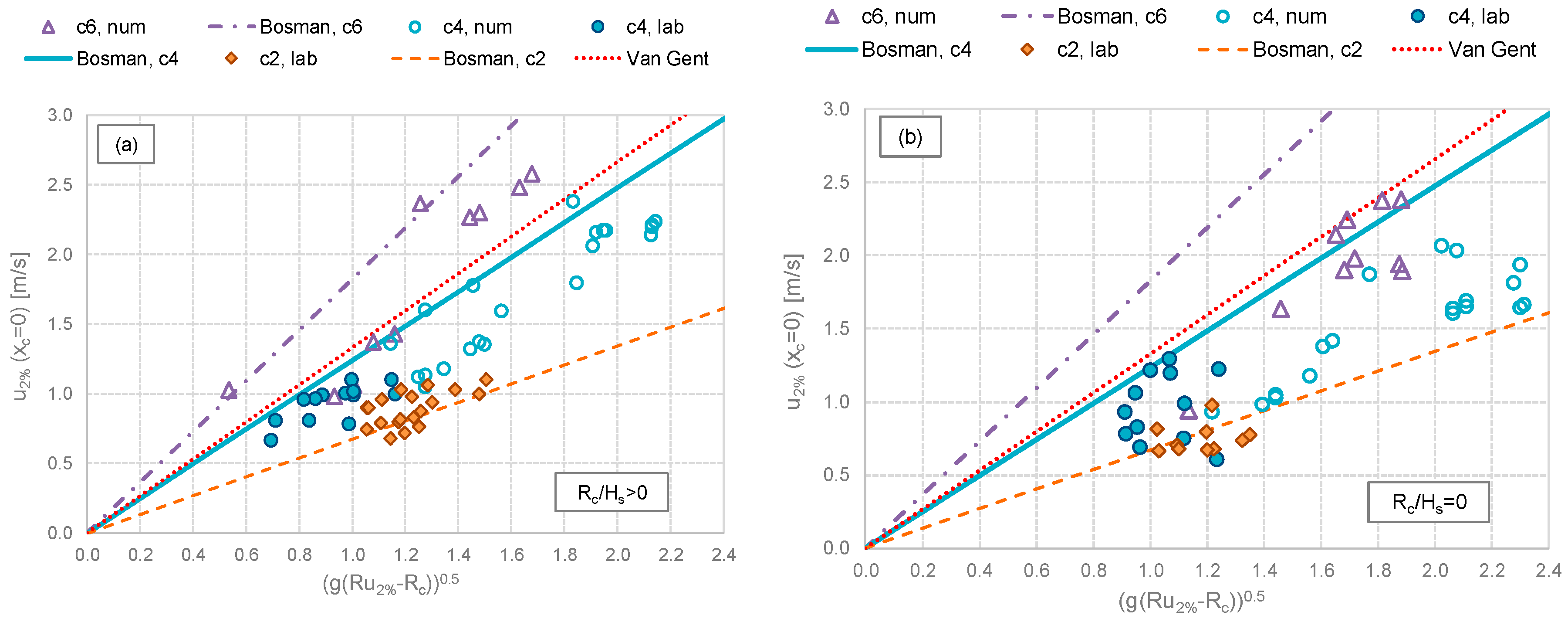
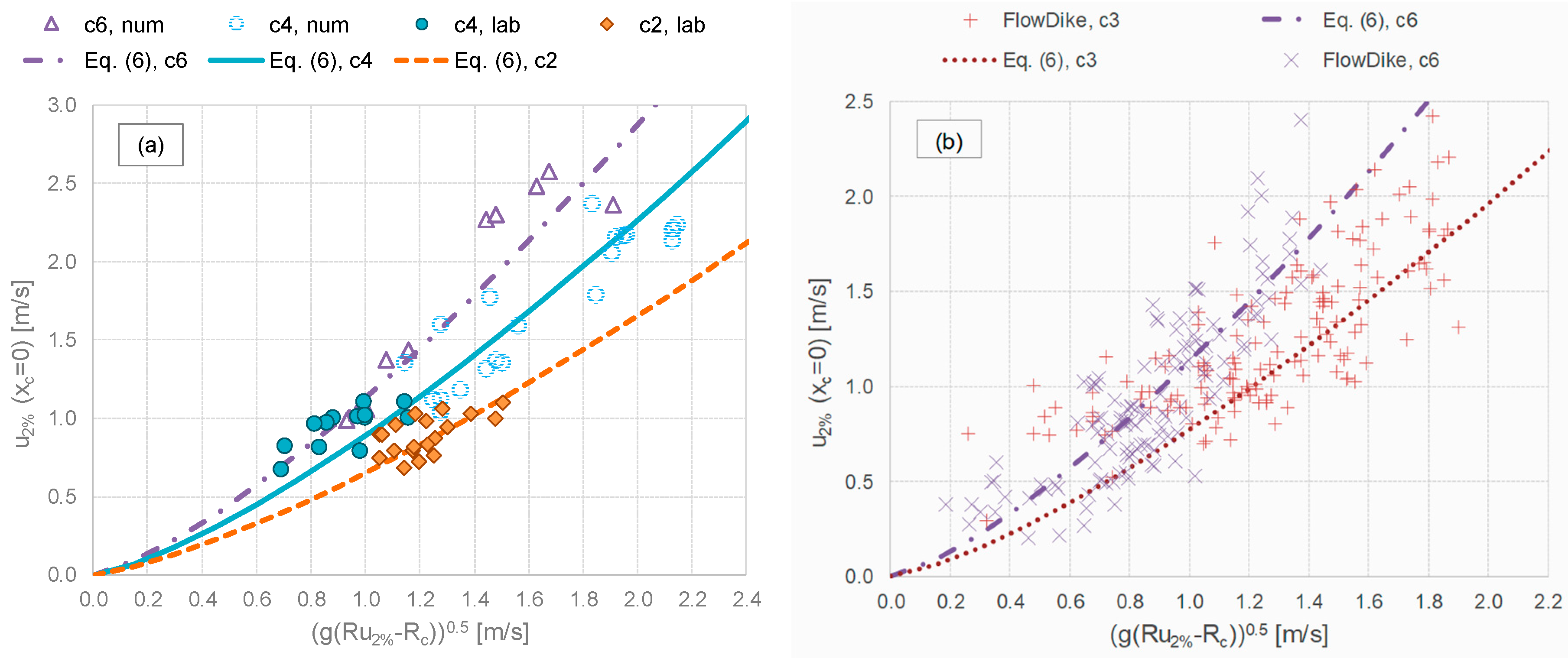
  • Similarly to h2%, the formula by Van Gent [5] (dotted line) gave an average estimation of the u2%-values, representing, respectively, an upper and a lower envelope for the data at c4 and c6. The data at Rc = 0 (panel b)—which are out of the range of validity of the formula—were significantly over-estimated by Van Gent.
  • The effect of cot(αoff) is still evident: the milder the slope, the higher u2%(xc = 0)—but slightly smoothed, with respect to h2%(xc = 0). With the exception of the data at c2, most of the data of u2% were over-predicted by the formulae by [8], by 30%–50% in case of Rc/Hs > 0 (filled-in points) and of 40%–80% in case of Rc/Hs = 0 (void points).
  • On average, the data at Rc/Hs = 0, tend to be lower than the data at Rc/Hs > 0 for the same value of the abscissa; i.e., (g∙(Ru,2% − Rc))0.5.
The discussion about these results, specifically regarding the discrepancy among formulae and u2% values and the effects of cot(αoff) and Rc/Hs, is given in the next Section 5.2.

5.2. Discussion of the Results

The overestimation given by the formulae by Bosman et al. [8] in case of u2%(xc = 0) can be explained considering the following three aspects.
First, Bosman et al. calibrated the coefficients cu based on the results of the previous experiments [4] and [5]. In those experiments, the measurements of u were obtained from micro-propellers placed at a fixed height over the structures. Therefore, the formulae were calibrated against punctual measures of u, while the values of u2% obtained from the new experimental and numerical modelling (and shown in Figure 10) were based on the average values of the velocities along the vertical above the structure crest. To further investigate this aspect, Figure 11 shows as example 2 instantaneous vertical profiles of u measured at D1 (i.e., approximately at xc = 0) during the test R00H05s3G15c4 conducted in the laboratory (Figure 11a) and reproduced with the numerical code (Figure 11b). Both the profiles refer to the instant of occurrence of the maximum flow depth h at D1 (i.e., around 0.38 m). Both the charts show a high variability of the u along the vertical: the vertically-averaged values of the u are 0.34 and 0.39 m/s for the laboratory and numerical test, respectively, with standard deviations of ±0.10 and ±0.05 m/s, and maximum values of u which are higher than the average of approximately 30% and 20%. This example indicates how much the vertical position of the instrument may affect the measured value of u, especially in case of laboratory tests, where the uncertainty related to the measurements is higher (as evident by comparing Figure 11a to Figure 11b).
Second, the discrepancy between flow velocities and wave celerities, c. Bosman et al. refitted the original values of the coefficients cu—which were originally calibrated by Schüttrumpf [4] on the measurements of u—to account for the higher values of the c observed for the tests. Based on the observation that, for the same test, c tended to be greater than u, Bosman et al. increased the values of cu from 1.37 to 1.64 to achieve a more cautious approach. The formulations of cu as functions of cot(αoff) further prompted by Bosman et al. were fitted again on the values of c instead of u.
Figure 12 provides the comparison among c and u2%-values for the new experimental dataset. The wave celerities have been computed using the procedure for the identification and coupling of the overtopping waves developed by references [36,37]. The procedure was applied to the time series of the h-signals registered at D1 and D3, providing as outputs, the time lags for the waves to propagate from D1 and D3. The c-values were computed from the time lags, known the distance D1–D3. Figure 12 shows that the c-values are indeed higher than the corresponding u2%, and the discrepancy among c and u tends to increase with increasing u.
These results are in line with the findings of Bosman et al. [8]. However, the present study followed the original work by Schüttrumpf [4] and the analyses of the overtopping flow characteristics were conducted based on the flow velocities.
Finally, the effect of Rc/Hs. The on-average lower u2%-values observed at Rc/Hs = 0 (Figure 10b) than at Rc/Hs > 0 (Figure 10a) are due to the different characteristics of the flow in the two freeboard conditions. When Rc/Hs > 0, the dike crest is located above the mean water level in the wave run-up area and the waves go overtop the dike crest during the crest phase exclusively, resulting, thus, in positive—i.e., in-shore directed—values of u at xc = 0. On the contrary, when Rc/Hs = 0, the dike crest level is situated exactly in line with the mean water level; i.e., in the middle between the wave run-up and run-down area. In such conditions, the waves can reach and overtop the dike crest during the through phase also, determining a flow in regard to the dike edge which is intermittently in-shore and off-shore directed, with values of u that area alternatively >0 and <0. This phenomenon is clearly evident in the example of Figure 13, which reports the frequency distribution of all the u-values measured with UVP at D1 for the same experimental test (H05s3G30c4) conducted at Rc/Hs = 0 (R00) and Rc/Hs = 1 (R10). In this example, there was a predominance of negative u-values in case of R00, while for R10, the distribution clearly shifted towards positive u-values. The different overtopping flow conditions and the resulting different distributions of the u-values affected, in turn, the values of u2%.

5.3. Refitting of the Formulae

Based on the analyses of the results, the following refitting of the literature formulae for the prediction of h2% and u2% at the dike off-shore edge (xc = 0) are proposed:
{ h 2 % ( x c = 0 ) = a h · ( R u 2 % R c ) b a h = 0.085 · cot   α o f f ;   b = 1.35 ,   for   R c H s 0
{ u 2 % ( x c = 0 ) = a u · [ ( g ( R u 2 % R c ) ) 0.5 ] b a u = 0.12 · cot   α o f f + 0.41 ;   b = 1.35 ,   for   R c H s > 0
Equations (5) and (6) follow the same form of Equations (3) and (4), respectively, but present a non-linear relationship between h2% and (Ru,2%Rc), and u2% and [g(Ru,2%Rc)]0.5 through the introduction of the power coefficient b = 1.35. The coefficients ch and cu of Equations (3) and (4) are, respectively, replaced by the new coefficients ah and au, whose formulations vary linearly with cot(αoff), as indicated in Equations (5) and (6). The dimensions of ah and au are, respectively, [m0.65] and [m0.65s−0.65].
Note that, while Equation (5) applies to Rc ≥ 0, Equation (6) is valid for Rc > 0 only. As discussed in Section 5.2, the values of u2% follow different trends with [g(Ru,2% − Rc)]0.5 at positive and at zero freeboard. Since no further data were available from the literature for check, no fitting was proposed for u2%(xc = 0) at Rc = 0.
The agreement between the new fitting and the experimental and numerical data is qualitatively shown in Figure 14a and Figure 15a for h2% and u2%, respectively, and quantitatively represented by the error indexes R2 and σ% reported in Table 6. This Table includes also the values of R2 and σ% associated to the application of Equations (3) and (4) to the new data obtained by considering the formulations of ch and cu [8].
In order to check the validity of the new fitting, Equations (5) and (6) were also applied to the prediction of h2%(xc = 0) and u2%(xc = 0) for some tests of the datasets FlowDike1 and FlowDike2 [38,39]. These tests involved 2D and 3D wave attacks against smooth dikes characterized by different values of Gc (0.6 and 0.7 m, model scale values) and of cot(αoff) (3 and 6, respectively in FlowDike1 and FlowDike2). The following tests from FlowDike1 and FlowDike2 were not considered for the analyses:
  • All the tests with missing records of either Ru2%, h2%(xc = 0) or u2%(xc = 0);
  • The tests giving zero or negative overtopping discharge (considered unreliable);
  • All the tests with wind velocity >10 m/s, as this fitting does not include the wind effect.
The values of h2%(xc = 0) and u2%(xc = 0) from the remaining tests are compared to Equations (5) and (6) in Figure 14b and Figure 15b, respectively. The quantitative assessment of the agreement between the FlowDike1 and FlowDike2 data and the new formulae are given in Table 6, that also includes the performance of Equations (3) and (4) for comparison.
Overall, both new and existing data seem to follow the same trend of the curves representing the new fitting, either in case of h2% (Figure 14) or of u2% (Figure 15). The best agreement is found between Equation (5) and the values of h2% from the numerical dataset, being that R2 = 0.996 and σ% = 4.1% (see Table 6). A larger scatter was observed for the other datasets, as indicated by the values of σ% ranging between 15% (new laboratory data of u2% and Equation (6)) and 51% (FlowDike2 data of u2% and Equation (6)). The relatively high values of σ% are caused by the intrinsic scatter associated to the data, especially to the FlowDike1 and FlowDike2 experiments, and do not necessarily indicate a poor agreement with the new fitting. This is confirmed by the values of σ% associated to the predictions by Equations (3) and (4), which are comparable or even higher to the σ% associated to the new fitting. On the contrary, Figure 14 and Figure 15 reveal that the new formulae provide a good, “average” representation of most of the data, which are randomly but symmetrically distributed around the curves following their trends. This qualitative analysis is confirmed and reinforced by the values of R2 of Table 6, which are always >0.72 and in six cases out of eight, even >0.80. Equations (3) and (4) provide a similar—but lower—performance on FlowDike1 and FlowDike2 data, while they give a worse representation of the new experimental and numerical data, as indicated by Figure 9 and Figure 10.
In conclusion, the new fitting by Equations (5) and (6) represents a more cautious alternative to that by Equations (3) and (4), respectively, also applying to steep slopes (cot(αoff) = 2, 3) and low freeboards. Its use is suggested especially in case of relatively high run-up levels, i.e., approximately for values of (Ru,2%Rc)/Hs > 2–2.5, which represent very severe surge conditions to catastrophic flooding scenarios.
The new formulae were applied in the following ranges: 0 ≤ Rc/Hs ≤ 4.0 and 0 < Rc/Hs ≤ 4.0 in case of Equation (5) and Equation (6), respectively; cot(αoff) = 2; 3; 4; 6; 0.72 ≤ ξm-1,0 ≤ 6.13; 0.035 ≤ Hs ≤ 0.22 m.

6. Evolution of Flow Characteristics along the Dike Crest

This Section focuses on the evolution of the flow depths and velocities between the dike off-shore and in-shore edges. Section 6.1 provides the comparison among the data of h2% and u2% and the literature formulae [7]. Section 6.2 and Section 6.3 are dedicated to an in-depth analysis of the values and trends of the flow velocities, with specific attention to the effects of the crest freeboard and wave breaking. Section 6.4 draws some conclusions about the analyses of the flow velocities, providing a few guidelines for practical use.

6.1. Comparison with Literature Formulae

The existing methods for the prediction of the evolution of flow depths and velocities along the crest of a smooth dike were developed starting from the physical and theoretical analysis by Schüttrumpf [4], which was based on experimental evidence and on these assumptions:
  • The dike crest is horizontal;
  • The vertical velocities can be neglected;
  • The pressure term is almost constant over the dike crest;
  • The viscous effects along the flow direction are small;
  • The bottom friction is constant over the dike crest.
Articles [4,7] describe the flow evolution of both h and u in terms of exponential decays along the dike crest, resulting in the following formulations:
h ( x c ) h ( x c = 0 ) = exp ( - c 3 x c G c ) ,   R c 0
u ( x c ) u ( x c = 0 ) = exp ( - f 2 · x c h ( x c ) ) ,   R c 0
where xc is the horizontal coordinate along the crest, h(xc) is the overtopping flow depth on the dike crest at the coordinate xc; u(xc) is the overtopping flow velocity on the dike crest at the coordinate xc; c3 is a dimensionless coefficient, varying according to the quantile used for h and u (50%, 10%, 2%); and f is the bottom friction coefficient.
The decay of h (Equation (7)) is due to the energy loss and to the deformation of the overtopping volume induced by the change of flow direction from the off-shore slope to the dike crest. The decay of u (Equation (8)) should be induced by the friction over the crest. However, as remarked by [7], the contemporary decay of u and h contradicts the continuity equation. In fact, the authors observed significant reductions of h (up to the 50%) but very modest changes of u, yielding to the conclusion that u was almost constant for the tested conditions; i.e., for a relatively short and smooth crest at zero freeboard and emerged conditions, Gc = 0.3 m and Rc ≥ 0. Therefore, for a smooth dike, the authors suggested the use of the (very low) value of f = 0.0058, which reduces u approximately 8%.
Later, small and large-scale model tests were carried out to check the validity of Equations (7) and (8) and to update the formulations [1,8,40]. Based on these results, the EurOtop manual [28] provides the following indications.
The flow thickness h decreases of approximately 1/3 with respect to the value at the off-shore edge; no new formulation is proposed in place of Equation (7).
The flow velocity u decays along the crest as a function of the wave length Lm-1,0, according to the following relationship:
u 2 % ( x c ) u 2 % ( x c = 0 ) = exp ( - 1.4 · x c L m - 1 , 0 ) ,   R c 0
Reference [28] warns about the potential inadequacy of Equation (9) in case of large crests (such as promenades).
Recently, a new analytical model [10] was proposed to describe the evolution of the maximum flow velocities (U) on the dike crest and landward slope. The model consists of two coupled formulae to be applied in sequence for the dike crest and the landward slope, respectively. The first formula still predicts the decay of U along the dike crest due to the bottom friction f:
U ( x c ) = 1 f x c 2 Q + 1 U ( x c = 0 ) ,   R c > 0
where based on the “momentary discharge Q;” i.e., the discharge calculated at the instant of occurrence of the maximum flow velocity U. The approach by article [10] gives also a formulation for the evolution of the “momentary layer thickness”, hU, derived from the continuity equation of Q, but no validation is given for this formula.
So far, no predicting method exists for the evolution of h and u in case of Rc < 0. Moreover, the formulae for u are verified against the off-shore and the in-shore values u(xc = 0) and u(xc = Gc) only. The numerical simulations (see Table 1) provide instead, continuous records of u and h between xc = 0 and xc = Gc for any crest emergence and submergence. Due to the limits of the laboratory equipment, the following analyses and discussion are principally based on numerical results: experimental evidence is available for the values of u and h corresponding to the UVPs; i.e., at D1, D2 and D3, for Rc/Hs ≥ 0 and dry landward conditions.
Following EurOtop [13,28], the quantiles 2% were considered in this study. Figure 16 illustrates the trends of h 2 %   ( x c ) h 2 % ( x c = 0 ) and u 2 %   ( x c ) u 2 % ( x c = 0 ) derived from the numerical results for different values of Rc/Hs. In case of Rc/Hs < 0, only tests in dry landward conditions were considered.
The flow thickness h2% (panel a) decays almost linearly with xc, showing a certain dependency with Rc/Hs. The decrease of h, ranging between 15 and 20% for Rc < 0, and being 35% for Rc/Hs = 1.5, is in agreement with EurOtop [28] but it is lower than the estimations of Equation (7), which would predict a decrease of approximately the 50%. The same decays were approximately found when comparing the values of h2%(D1) with the corresponding values of h2%(D3) both in experiments and in simulations.
Based on the numerical and experimental results and on the indications of EurOtop [28], it is, therefore, suggested to use Equation (7) for h2% by adopting the following values of the coefficient c3:
{ c 3 = 0.35 ,   if   R c 0 c 3 = 0.18 ,   if   R c < 0 ,   for   dry   landward   conditions   only
The comparison among the predictions of h2%(xc = Gc) derived from the application of Equation (7) with the coefficients given in Equation (11) and the corresponding numerical values led to standard deviations σ and coefficients of determination R2, respectively equal to 0.06 and 0.93 for Rc ≥ 0 and to 0.09 and 0.96 for Rc < 0. For Rc < 0 in wet landward conditions, i.e., fully submerged or breached dikes, no significant changes of the values of h were detected along the crest.
The trend of u2% along the dike crest (Figure 16b) is significantly different for tests at positive or negative freeboard. In case of Rc ≥ 0, a slight decay was observable until xc/Gc ≈ 0.4, while the trend seems to invert around xc/Gc = 0.6 and u increases up to approximately the same value of the crest beginning; i.e., u(xc = Gc) ≈ u(xc = 0). In case of Rc < 0, u monotonically increases with an apparent quadratic function of xc from the beginning to the end of the dike crest. The different trends of u were, therefore, investigated separately for positive and negative freeboards in Section 6.2 and Section 6.3, respectively.

6.2. Flow Velocities at Zero and Positive Crest Freeboard

The initial decay and subsequent increasing trend of u for xc/Gc > 0.4–0.5 was already observed by Guo et al. [17] in case of numerical tests with Rc ≥ 0. The combination of decreasing flow thicknesses (Figure 14a) and increasing flow velocities (Figure 14b) along the dike crest fulfills the continuity and the momentum balance equations, accounting also for the (small) effect of the friction. However, it is clearly in opposition with the existing approach by Schüttrumpf and Oumeraci [7] that is based on the approximation of the Navier–Stokes equations. Schüttrumpf and Oumeraci highlighted indeed, that their approach contradicts the instantaneous continuity equation, but they found experimental evidence of the decay of u and pointed out that the continuity equation is globally fulfilled by considering the time-integral of the product of u by h. Guo et al. [17] argued that the discrepancy between the results of their numerical modelling and the equations by Schüttrumpf and Oumeraci can be explained by a number of elements, such as (i) the dynamics of the overtopping flow over the dike crest and the shape of the water front; (ii) the effect of the air entrainment; and (iii) the limitations imposed by the assumptions by Schüttrumpf and Oumeraci; specifically, the approximation of the boundary layer and the adoption of flow-depth integrated velocities. These aspects are analyzed in detail in the following Section 6.2.1 and Section 6.2.2.

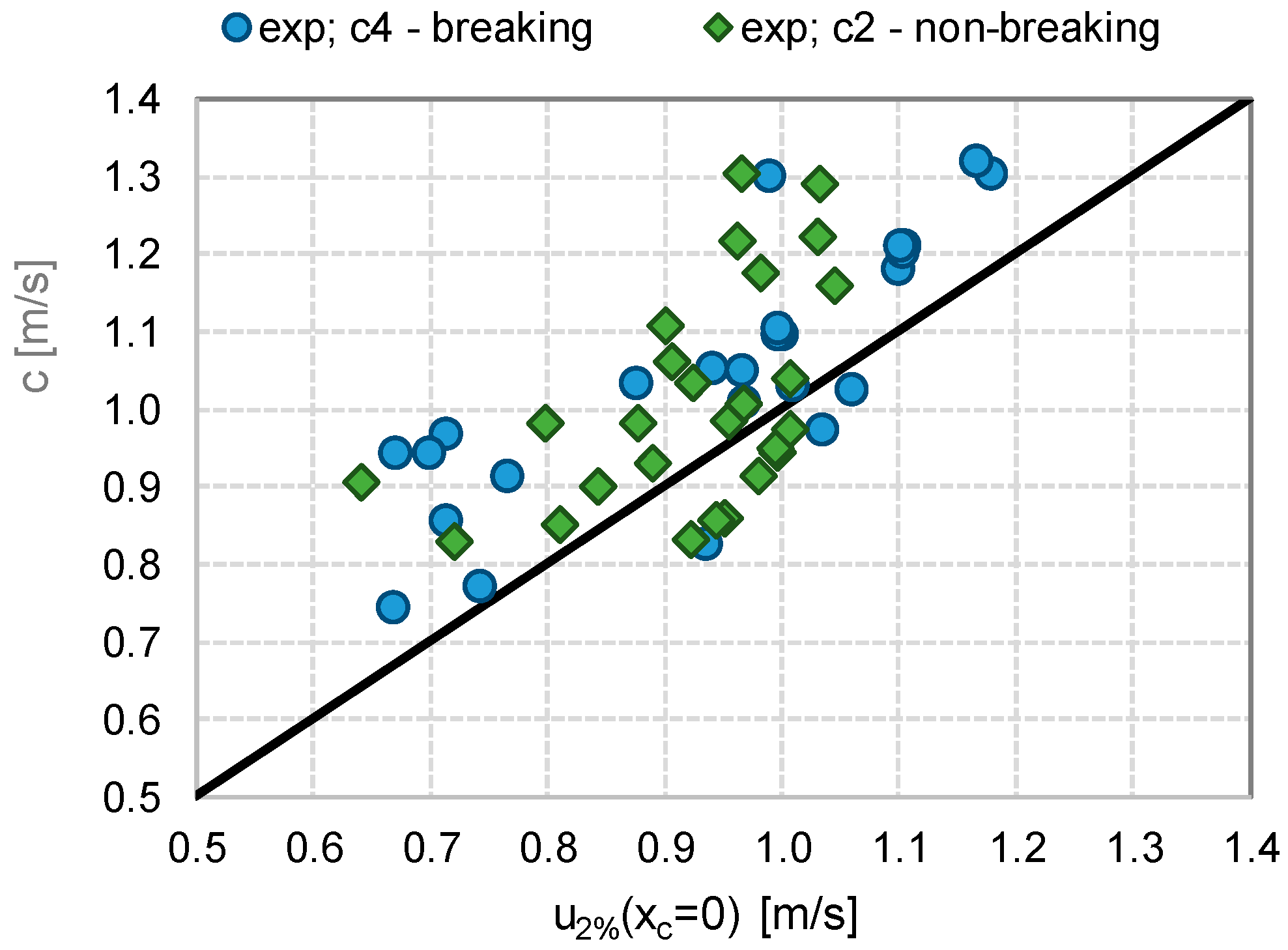
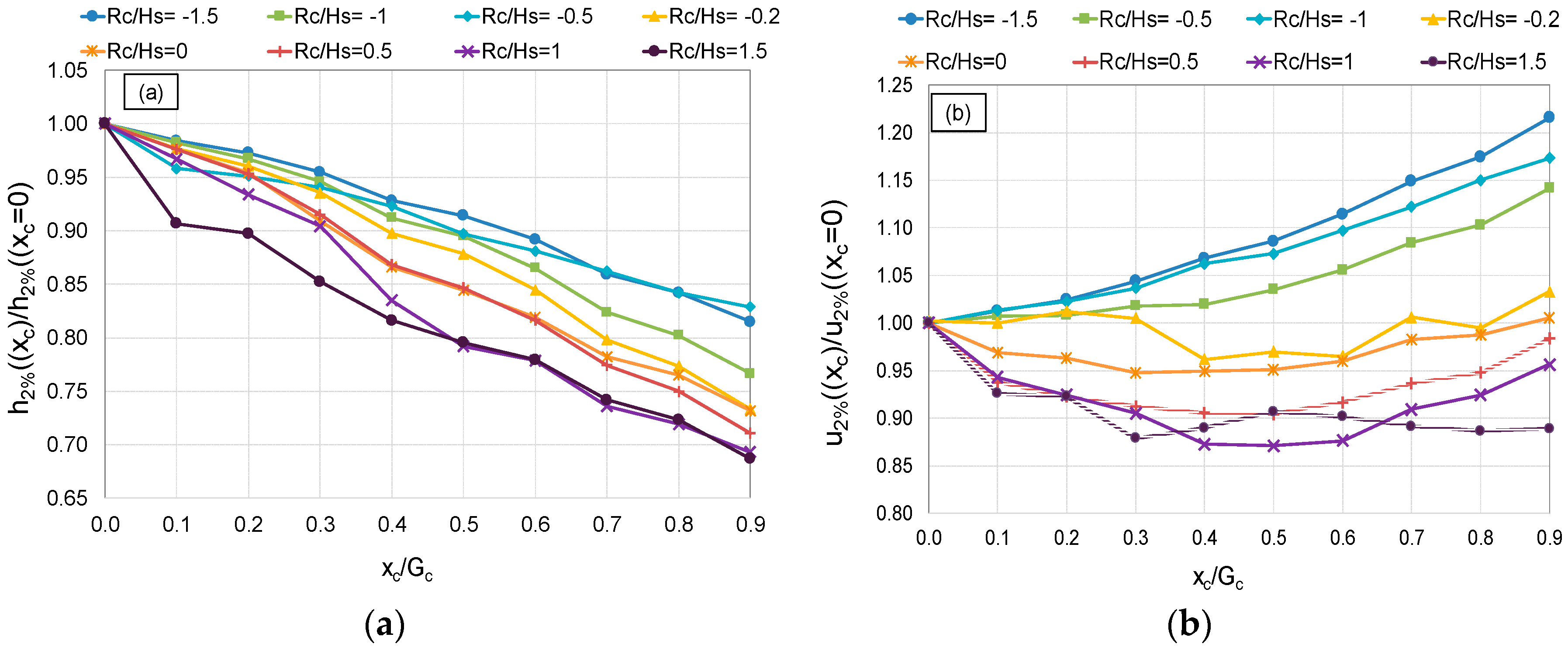
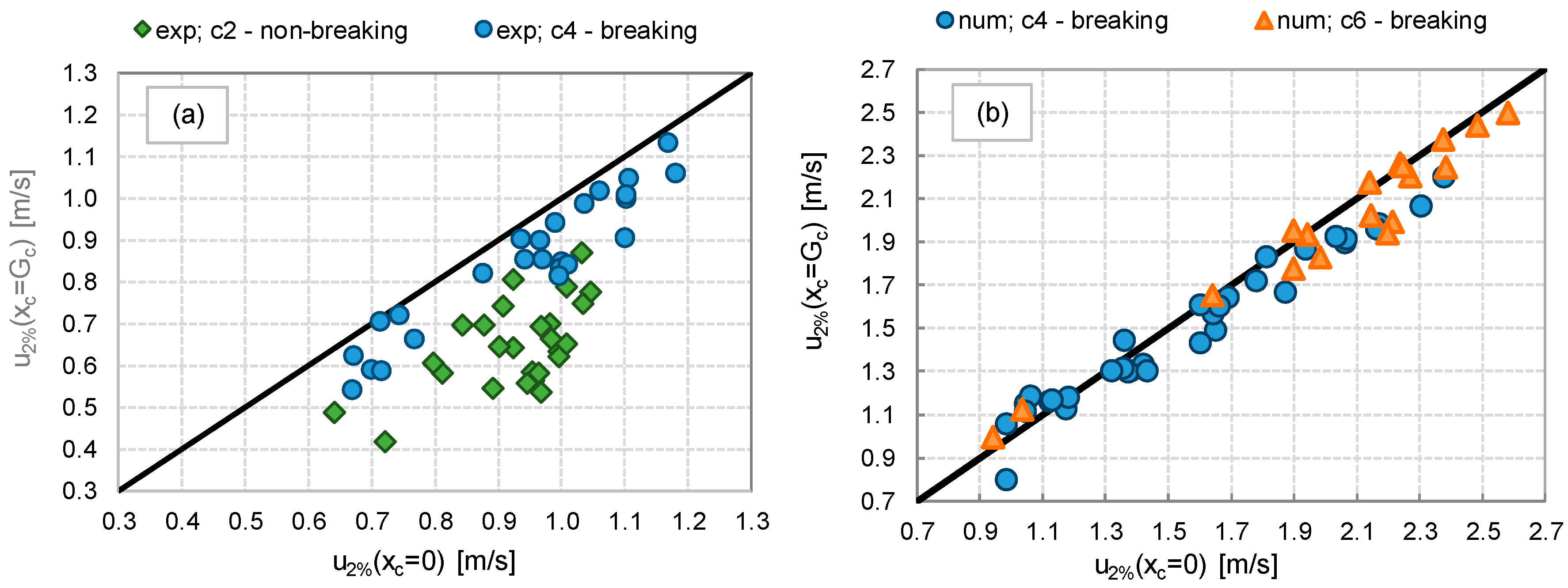
6.2.1. Effect of the Wave Breaking

One of the main points raised by Guo et al. [17] to justify the different trends of u along the dike crest with respect to Equation (8) regards the different dynamics of propagation of the breaking and non-breaking waves over the dike crest. When the wave reaches the dike crest in breaking or fully-broken conditions (see Figure 15), it has already dissipated most of its energy, and the flow over the dike crest is highly turbulent and is characterized by a large amount of air pockets entrapped in the water tongue. The air entrainment may induce significant differences between the results of physical, numerical and theoretical modelling due to the different approaches for the assessment of the flow velocity. In the laboratory, the UVPs provide measurements of the instantaneous vertical profiles of u, which can be severely affected by the presence of air pockets in the water column as the sonic impulse of the UVP is interrupted when travelling across air. The numerical code can calculate the u-values of the water phase exclusively, neglecting the air-phase, leading, therefore, to potential over-estimation of the u-values. Finally, Schüttrumpf and Oumeraci [7] considered a steady-flow boundary layer and flow-depth averaged velocities, hence evaluating the maximum u-values at the free surface. It is evident that these assumptions hold no more in case of broken waves in turbulent flow, where the maximum u is found close to the dike surface.
As an example, Figure 17 show two frames of the same overtopping event derived from the physical (left) and numerical (right) modelling of the test R00H05s3G30c4. The color map of Figure 17b illustrates the flow velocity field from computations. In both panels of Figure 17a,b, the flow propagates on the dike crest after the wave breaking has already occurred along the dike slope. In such conditions, the overtopping flow is similar to a weir-like stream governed by the outfall in-shore condition. Due to the modest or null friction, the value of u2% hardly decays while propagating along the dike crest. Similarly to the results of Guo et al., the numerical model suggests that the flow velocity tends on the contrary to accelerate. The shape of the overtopping tongue is correctly represented by the numerical code (Figure 17b). However, the large amount of air pockets characterizing the flow in the laboratory (Figure 17a) cannot be captured by the mono-phase numerical code.
A completely different situation occurs in case the wave reaches the dike crest before breaking. Guo et al. [17] observed that, in such conditions, the overtopping tongue overtops and jumps above the dike off-shore edge, hitting the crest around or just before its middle section (see Figure 18). The section of the impinging jet determines, thus, a sharp modification of the velocity field along the dike crest:
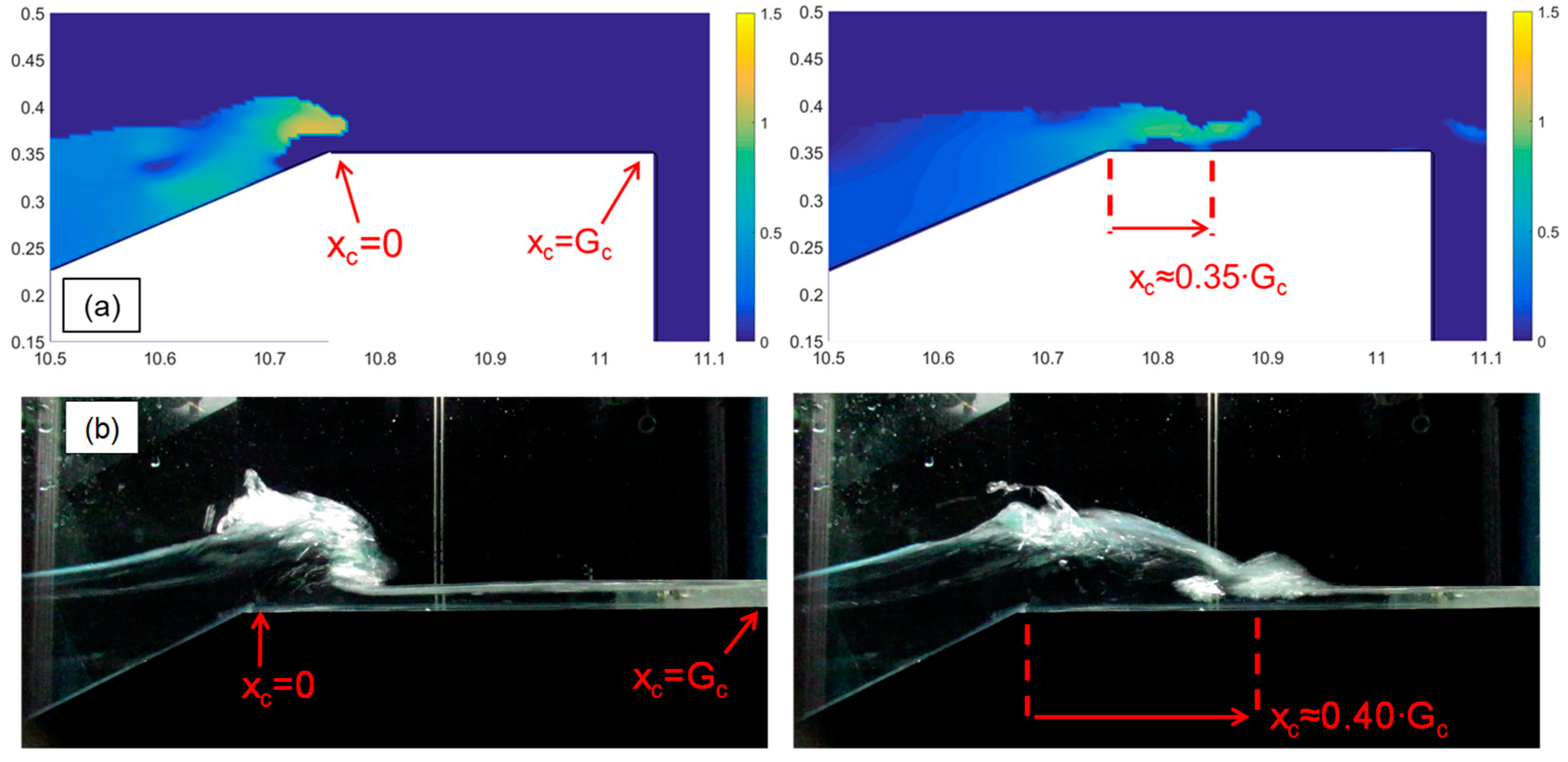
  • From the off-shore edge to the impinging jet section, xc ≈ [0; 0.4∙Gc], the overtopping tongue dissipates its energy in the change of direction from the up-rush along the seaward slope to the horizontal stream over the crest;
  • Corresponding to the section of the impinging jet (xc ≈ 0.4∙Gc), the wave front hits violently against the dike crest surface and breaks; this section is subjected to the maximum impact (wave pressure), and as a consequence of the momentum balance equation, to the minimum velocity; the section is, therefore, associated to the maximum stress and possibly to the maximum scour risk;
  • In the second half of the dike crest, xc ≈ [0.5∙Gc; Gc], the overtopping flow velocity tends to accelerate into a supercritical stream for the free-outfall boundary condition at the landward edge, while the potential energy accumulated at the hit turns into kinetic.
In the present work, we found numerical and experimental confirmation of the results by Guo et al. [17]. Figure 18a,b provides two consecutive frames of an impinging jet observed within the same numerical (18a) and experimental (18b) test R00H05s3G30c2. Both the numerical and the experimental frames show the wave overtopping the dike off-shore edge before breaking and impinging on the crest around its middle section, xc ≈ [0.35; 0.4∙Gc]. Based on the color map of Figure 16a, u is maximal at the off-shore edge and decelerates while the wave propagates along the dike crest. At the impinging section, the u-value is minimal, correspondingly with the crest surface, and it starts increasing again after the impact. The result of this process is the decreasing/increasing trend of u2% leading to values of u2%(xc = Gc) ≈ u2%(xc = 0), as shown in Figure 16b.
Figure 18a,b also shows the presence of air pockets entrapped in the water tongue, especially in the area beneath the surging breaker immediately preceding the impinging section. The air entrainment is still thought to be a concurrent cause of the discrepancies between numerical and experimental results and the theoretical approach by Schüttrumpf and Oumeraci [7], as already identified by Guo et al. [17].
The different trends of u associated to the different breaker types affect the value of u2% at xc = Gc, which in the practice represents one of the most relevant parameters, as it governs the down-wash streaming in the inland area. Figure 19 compares the values of u2%(xc = Gc) to the corresponding values of u2%(xc = 0) obtained from the experimental (Figure 19a) and numerical tests (Figure 19b) for the different breaking or non-breaking conditions. All the numerical tests (at Rc/Hs ≥ 0) represent waves reaching the dike crest in breaking (cotαoff = 4) or broken (cotαoff = 6) conditions, while the experimental tests present both non-breaking (cotαoff = 2) and breaking (cotαoff = 4) wave conditions.
From Figure 19 it is evident that u2% effectively decays from xc = 0 to xc = Gc only in case of c2; i.e., of non-breaking waves (green diamonds). The average decay was of approximately the 30%, ranging between 13% and 45%. The variability of the decay rate was due to the different combinations of crest widths, freeboard conditions, wave steepness and wave heights. However, no explicit or systematic relationship was found between the decay rate and any of the parameters Gc, Rc/Hs, Hs/Lm−1,0 and Hs. The absence of a direct link between the decay rate and Gc can be explained with the small friction determined by the smooth dike surface and by the limited value of Gc. This result is in agreement with the synthesis by EurOtop [13,28], where a specific indication of negligible decay for flow depths larger than 0.1 m and Gc around 2–3 m is reported.
In cases of c4 (blue circles) and c6 (orange triangles), both the numerical and the experimental results indicate that the decay rates are significantly reduced, being on average of 10% and ranging between −7% and 28%. These results—which are in line with the average trends of Figure 18b—suggest that in case of breaking or broken wave conditions, the decay of u2% along the dike crest is almost negligible, and in some cases u2%(xc = Gc) might result even greater than u2%(xc = 0), as already observed by Guo et al. [17]. Generally, the phenomenon of the increasing velocities from xc = 0 to xc = Gc is more frequently observed with the numerical code (Figure 19b), which also tends to give a slightly lower decay rates with respect to the physical experiments (Figure 19a).

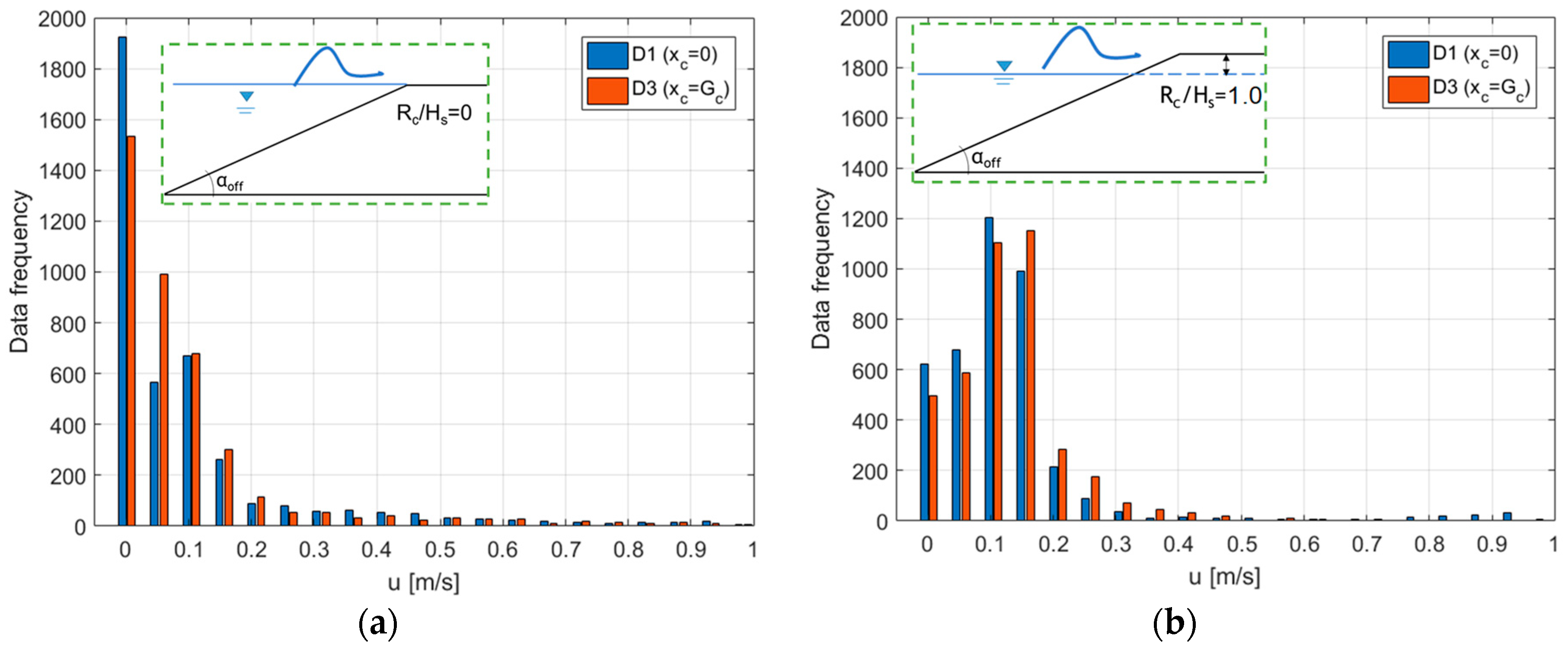
6.2.2. Effect of the Crest Emergence

In case of Rc ≥ 0, the decay rate of u2% from xc = 0 to xc = Gc. was not directly correlated to Rc/Hs (see Section 6.2.1 and Figure 16b). Nevertheless, it was observed that the statistical distribution of the flow velocities was significantly different in cases of Rc/Hs = 0 and Rc/Hs > 0. To illustrate those outcomes, Figure 20 shows the frequency histograms of the instantaneous depth-averaged u-values measured during an example test case from the laboratory experiment H05s3G30c4 conducted at Rc/Hs = 0 (Figure 20a) and Rc/Hs = 1.0 (Figure 20b). In both panels of Figure 20a,b, the histograms are provided for the values of u recorded at both D1 (blue shading) and D3 (orange shading); viz., at xc = 0 and xc = Gc, respectively. The probability density function (pdf) for Rc/Hs = 0 (Figure 20a) presents a sharp peak corresponding of the lowest values of u (the mode is around ≈0.03 m/s for both xc = 0 and xc = Gc); then it decreases almost monotonically with the increasing u-values. The distribution for Rc/Hs = 1.0 (Figure 20b) was more flat and symmetrical, showing increasing and decreasing data frequencies for values of u, respectively, lower and greater than the mode, which is ~0.10 m/s for xc = 0 (blue bars) and ~0.10 m/s for xc = Gc (orange bars). The different mode values in case of Rc/Hs = 1.0 indicate that higher values of u are more frequently detected at D3 than at D1 (i.e., the distributions of u at D3 are shifted towards higher values than the distributions at D1); i.e., at xc = Gc rather than at xc = 0. In other terms, the flow more frequently accelerates than decelerates along the dike crest. This phenomenon is not detectable at Rc/Hs = 0 (Figure 20a).
From a practical point of view, the analysis of Figure 20 suggests that:
  • On average, the flow velocities at both the dike off-shore and in-shore edges are higher at Rc/Hs > 0 than at Rc/Hs = 0, as already observed for the extreme percentiles u2% reported in Figure 10;
  • In case of Rc/Hs > 0, the u-values are more narrowly distributed around the mode, showing a lower variability with respect to the case at Rc/Hs = 0;
  • At Rc/Hs > 0, the flow more frequently accelerates than decelerates from xc = 0 to xc = Gc, in line with the discussion proposed in Section 6.2.1.
The same results here illustrated for the example case of Figure 20 were found for most of the conditions tested.

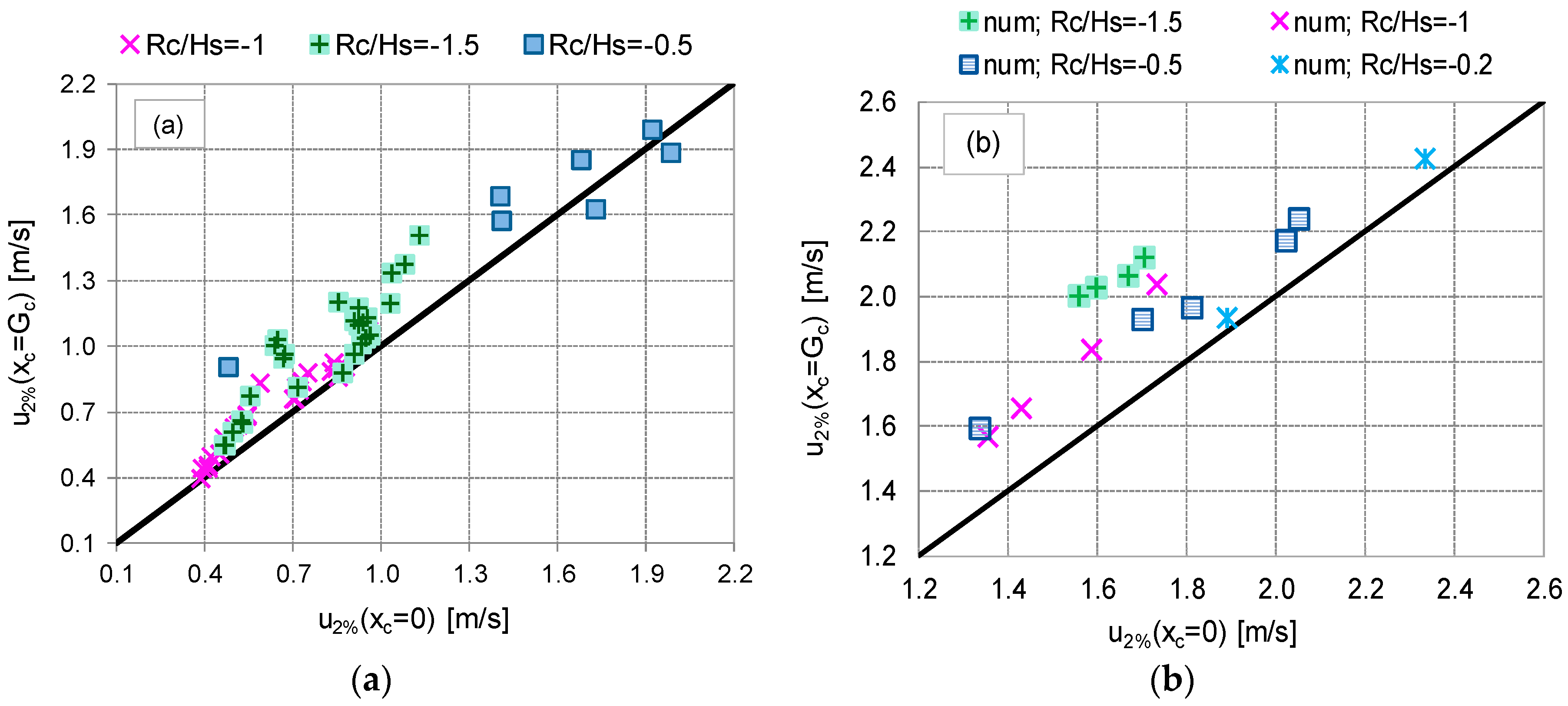
6.3. Flow Velocities at Negative Freeboard

The phase of decay of u2% from xc = 0 to xc ≈ 0.4Gc observed for Rc/Hs ≥ 0 no longer occurred at Rc < 0 (see Figure 16b), because the energy dissipation induced by the wave breaking and jumping against the dike crest (see Figure 18 and Section 6.2.1) was reduced or nullified by the presence of the water over the crest. Indeed, at Rc < 0, a weir-like constant supercritical flow was established over the dike crest due to the hydraulic gradient between the dike off-shore and in-shore edges. The free outfall condition at the landward slope governed the overflow process, inducing the flow to accelerate and resulting into values of u(xc = Gc) greater than the values u(xc = 0). Figure 16b shows, indeed, a monotonic increasing trend of u2% from xc = 0 to xcGc for all the cases at Rc < 0.
In many cases, the water layer above the dike crest prevents the wave from breaking at all. For this reason, the effect of the wave breaking presented and discussed for Rc/Hs ≥ 0 no longer applies. On the contrary, a sharp effect of Rc/Hs was observed, as the increased rate of u2% increased with the crest submergence. Such an effect was already evident from the average trends of Figure 16b and is displayed by Figure 21, which compares the numerical values of u2%(xc = 0) with the corresponding values u2%(xc = Gc) for all the available numerical tests at Rc < 0 in wet (panel a) and dry (panel b) landward conditions. In that figure, the data are clustered on different levels above the bisector line according to the values of Rc/Hs: the lower the value of Rc/Hs, the farther the data from the bisector; i.e., the lower the Rc/Hs, the larger the ratio u2%(xc = Gc)/u2%(xc = 0). On average, the values of u2%(xc = Gc)/u2%(xc = 0) ranged from 5% to 30% for Rc/Hs ranging from −0.2 to −1.5 in dry landward conditions. Similar results were observed for the wet landward conditions, though the increase of u2% from xc = 0 to xc = Gc seemed to be more modest (up to 20%–25%) and not sharply related to Rc/Hs. This was probably due to the presence of the water on the landward side, which determines lower hydraulic gradients between the off-shore and in-shore edges, and consequently, more modest flow acceleration.
The combined trends of increasing velocities and decreasing thicknesses along the crest fulfill the continuity and the momentum balance equations. The contradiction with the theory [7] holds no more, as the tested conditions by the authors were limited to Rc > 0.

6.4. Remarks on the Flow Velocities and Design Recommendations

In agreement with Guo et al. [17], the numerical and experimental results led to the following general remarks about the evolution of the flow velocities along the dike crest.
For smooth surfaces the friction effect is negligible. The decay of u was observed only for very short crest widths for Rc > 0; for larger crests and/or negative freeboards, the application of the existing formulae (Equations (8) or (9)) might lead to incautious estimates.
For a conservative approach, it is suggested to neglect any decay of u along the crest in emerged conditions and to assume that u(xc = 0) = u(xc = Gc).
In case of Rc ≥ 0 and non-breaking waves, the minimum or zero velocity is found roughly around the middle section of the dike crest, where the imping jet hits the dike surface, and therefore, the highest loads and stresses are concentrated in this area. Based on this finding, the section subjected to the impinging jet can be considered the most exposed to the risk of scour. That outcome may result in practical interest in the case of permeable structures, and can be combined to the analyses of van der Meer et al. [40], who correlated the start of the scour to the occurrence of a given critical flow velocity.
For Rc < 0, the maximum flow velocities are found at the dike in-shore edge. This may result in higher downwash velocities along the dike landward slope and in the landward area. Therefore, it is advised to increase, by approximately 20%, the value of u at the in-shore edge with respect to the value at the off-shore edge (see Figure 16b and Figure 21).
It is important to remark that the analysis of the flow at Rc < 0 is available from numerical modelling only and that for Rc ≥ 0, the experimental data relate to punctual measurements of h and u in regard to the dike crest edges and its middle section.

7. Conclusions

A new database of 60 experimental and 94 numerical tests on wave overtopping against smooth trapezoidal dikes characterized by various slopes, crest levels and landward conditions was created. Overall, the tested configurations consisted of three off-shore slopes (cot(αoff) = 2, 4 and 6), relative crest freeboards in the range Rc/Hs = [−1.5; 1.5] and two crest widths Gc (3 and 6 m, in prototype units). The combinations of Hs/Lm-1,0 and cot(αoff) values were such to determine both breaking (ξm−1,0 ≤ 2) and non-breaking (ξm−1,0 > 2) wave conditions within both the numerical and the experimental tests.
The consistency of the new data was checked by comparing the values of the average overtopping discharge (q) and of the wave reflection coefficient (Kr) resulting from the new laboratory and numerical tests, with the corresponding predictions obtained from consolidated methods available from the literature ([28] for q; [34] for Kr; the artificial neural network by [32,33] for both q and Kr). The numerical model was validated by reproducing a subset of 12 experimental tests and by comparing the results in terms of: q, Kr, maximum and mean water depths (h) envelopes and extreme flow depths and velocities (h2% and u2%) across the dike crest.
The analysis of the values of h2% and u2% at the dike off-shore edge (xc = 0) and the comparison with the existing predicting methods [4,5,8] led to the prompting of two new formulations, Equations (5) and (6). These formulae were conceived i) to achieve a better accuracy in the representation of the data; ii) correct some incautious underestimations or excessive overestimations associated to the existing formulae; and iii) extend the field validity of the existing formulae to structures with cot(αoff) = 2 and Rc = 0. Equations (5) and (6) follow the same formulation of the existing methods (Equations (3) and (4)) but represent a non-linear increase of h2%(xc = 0) and u2%(xc = 0) with (Ru,2%Rc) and (g∙(Ru,2%Rc))0.5, respectively. Equations (5) and (6) propose also two new coefficients ah and au, which are proportional to cot(αoff). The ranges of validity of the method are: cot(αoff) = 2–6, ξm-1,0 = 1–4 and Rc ≥ 0 for h2%(xc = 0) (Equation (5)); and Rc > 0 for u2%(xc = 0) and smooth structures, i.e., γf = 1 (Equation (6)).
Equations (5) and (6) were calibrated on numerical and experimental data for modest wave run-up values corresponding to the typical working conditions of the coastal defense structures ((Ru,2%Rc)/Hs < 2). Higher run-up heights were also modelled with the numerical code to analyze more severe or catastrophic scenarios ((Ru,2%Rc)/Hs > 2–2.5) in a climate change situation. The validity of Equations (5) and (6) were checked against the two sets of experiments, FlowDike1 and FlowDike2 [39,40], on dikes with cot(αoff) = 3 and 6. The new formulae are characterized by at least the same accuracy of the existing methods when applied to FlowDike1 and FlowDike2, while they provide a remarkably better representation of the new experimental and numerical data.
The trends of h2% and u2% along the dike crest, i.e., from the off-shore (xc = 0) to the in-shore (xc = Gc) edge, were analyzed in detail from the numerical model at any crest emergence (−1.5 ≤ Rc/Hs ≤ 1.5) and for both dry, landward conditions. The numerical results are supported by experimental evidence in correspondence of xc = 0, xc ≈ 0.5 and xc = Gc and for values of Rc/Hs ≥ 0 and dry landward conditions. The analysis resulted in the following criteria for design application.
For each structure slope, crest freeboard and wave attack condition (wave heights and periods), the flow thickness h monotonically decreases from xc = 0 to xc = Gc. The decay of h is strictly dependent on the crest freeboard, varying approximately between the 20% and the 35% for over-washed (Rc/Hs = −1.5) and for emerged (Rc/Hs = 1.5) conditions respectively. To account for the effect of Rc/Hs, a new coefficient c3 for the decay formulation of h was proposed in Equation (10). For submerged dikes (Rc < 0 and wet landward conditions), the decay of h is almost negligible.
The effect of the friction along the crest on the flow velocity u is negligible in case of smooth dikes, in agreement with the EurOtop manual [13,28]. The trends of u are instead significantly influenced by Rc and by the wave breaking or non-breaking conditions.
For Rc/Hs ≥ 0 and non-breaking wave conditions, u decreases in the first part, reaches a minimum around the half of the crest, in accordance with the impinging jet hitting the dike surface, and then, increases in the second part, being that the values of u at the landward edge are approximately equal to the seaward edge. The section subjected to the impinging jet is the most exposed to the risk of scour. For a conservative approach, in case of Rc/Hs ≥ 0 it is suggested to assume u(xc = 0) = u(xc = Gc), while the use of the decay trends for u (Equation (8)) is discouraged.
For Rc/Hs ≥ 0 and breaking or broken waves, u hardly changes along the dike crest. The overtopping flow is governed by the free-outfall boundary condition at the dike off-shore edge, which determines a supercritical accelerated weir-like flow, resulting in values of u(xc = Gc) which may be even higher than u(xc = 0).
Based on numerical results only, for Rc/Hs < 0 u increases along the crest, and its growth rate increases by increasing the submergence, up to approximately the 30% for Rc/Hs < −1, both in the case of wet and dry landward conditions. Overall, it is suggested to assume a value of u at xc = Gc which is increased of the 20% with respect to the value at xc = 0.

Author Contributions

Conceptualization, S.M.F., G.P. and B.Z.; formal analysis, S.M.F., M.G.G. and M.G.; investigation, G.P. and B.Z.; data curation, S.M.F., M.G.G. and M.G.; writing—original draft preparation, S.M.F.; writing—review and editing, M.G.G. and B.Z.; supervision, B.Z.

Funding

This research was funded by the Horizon 2020 project BRIGAID (“BRIdging the GAp for Innovations in Disaster resilience,” www.brigaid.eu), grant number 700699.

Acknowledgments

The first author would like to express her sincere gratitude to Jentsje W. van der Meer for providing his own data and his analyzed results on the FlowDike experiments that we used for the validation of the new fitting. The support of the European Commission through the Horizon 2020 project BRIGAID (“BRIdging the GAp for Innovations in Disaster resilience,” www.brigaid.eu) is gratefully acknowledged.

Conflicts of Interest

The authors declare no conflict of interest.

References

  1. Van der Meer, J.W.; Hardeman, B.; jan Steendam, G.; Schuttrumpf, H.; Verheij, H. Flow depths and velocities at crest and inner slope of a dike, in theory and with the Wave Overtopping Simulator. In Proceedings of the ICCE 2010 (ASCE), Shanghai, China, 30 June–5 July 2010. [Google Scholar]
  2. Van der Meer, J.W.; Bernardini, P.; Snijders, W.; Regeling, E. The wave overtopping simulator. In Proceedings of the 30th ICCE 2006, San Diego, CA, USA, 3–8 September 2006; Volume 5, pp. 4654–4666. [Google Scholar]
  3. Sumer, B.M.; Fredsøe, J.; Lamberti, A.; Zanuttigh, B.; Dixen, M.; Gislason, K.; Di Penta, A.F. Local scour at roundhead and along the trunk of low crested structures. Coast. Eng. 2005, 52, 995–1025. [Google Scholar] [CrossRef]
  4. Schüttrumpf, H. Wellenüberlaufströmung bei See-Deichen. Ph.D. Thesis, Technical University Braunschweig, Braunschweig, Germany, 2001. [Google Scholar]
  5. Van Gent, M.R. Wave overtopping events at dikes. In Proceedings of the 28th ICCE 2002, Wales, UK, 7–12 July 2002; Volume 2, pp. 2203–2215. [Google Scholar]
  6. Schüttrumpf, H.; van Gent, M.R. Wave overtopping at seadikes. Coast. Struct. 2004, 2003, 431–443. [Google Scholar]
  7. Schüttrumpf, H.; Oumeraci, H. Layer thicknesses and velocities of wave overtopping flow at sea dikes. Coast. Eng. 2005, 52, 473–495. [Google Scholar] [CrossRef]
  8. Bosman, G.; Van der Meer, J.W.; Hoffmans, G.; Schüttrumpf, H.; Verhagen, H.J. Individual overtopping events at dikes. In Proceedings of the 31st ICCE 2008, Hamburg, Germany, 31 August–5 September 2008; pp. 2944–2956. [Google Scholar]
  9. Zanuttigh, B.; Martinelli, L. Transmission of wave energy at permeable low-crested structures. Coast. Eng. 2008, 55, 1135–1147. [Google Scholar] [CrossRef]
  10. Van Bergeijk, V.M.; Warmink, J.J.; Van Gent, M.R.A.; Hulscher, S.J.M.H. An analytical model of wave overtopping flow velocities on dike crests and landward slopes. Coast. Eng. 2019, 149, 28–38. [Google Scholar] [CrossRef] [Green Version]
  11. Mares-Nasarre, P.; Argente, G.; Gómez-Martin, M.E.; Medina, J.R. Overtopping layer thickness and overtopping flow velocity on mound breakwaters. Coast. Eng. 2019, 154, 103561. [Google Scholar] [CrossRef]
  12. Hughes, S.A.; Nadal, N.C. Laboratory study of combined wave overtopping and storm surge overflow of a levee. Coast. Eng. 2009, 56, 244–259. [Google Scholar] [CrossRef]
  13. Pullen, T.; Allsop, N.W.H.; Bruce, T.; Kortenhaus, A.; Schüttrumpf, H.; van der Meer, J.W. EurOtop. European Manual for the Assessment of Wave Overtopping. August 2007. Available online: www.overtopping-manual.com (accessed on 22 October 2019).
  14. Raosa, A.N.; Zanuttigh, B.; Lara, J.L.; Hughes, S. 2DV VOF numerical modelling of wave overtopping over overwashed dikes. Coast. Eng. Proc. 2012, 1, 62. [Google Scholar] [CrossRef]
  15. Formentin, S.M.; Zanuttigh, B.; van der Meer, J.W.; Lara, J.L. Overtopping flow characteristics at emerged and over-washed dikes. Coast. Eng. Proc. 2014, 1, 7. [Google Scholar] [CrossRef]
  16. Lara, J.L.; Ruju, A.; Losada, I.J. Reynolds Averaged Navier-Stokes modelling of long waves induced by a transient wave group on a beach. R. Soc. A 2011, 467, 1215–1242. [Google Scholar] [CrossRef]
  17. Guo, X.; Wang, B.; Liu, H.; Miao, G. Numerical simulation of two-dimensional regular wave overtopping flows over the crest of a trapezoidal smooth impermeable sea dike. J. Waterw. Port Coast. Ocean 2014, 140, 04014006. [Google Scholar] [CrossRef]
  18. Formentin, S.M.; Zanuttigh, B. A new method to estimate the overtopping and overflow discharge at over-washed and breached dikes. Coast. Eng. 2018, 140, 240–256. [Google Scholar] [CrossRef]
  19. Zelt, J.A.; Skjelbreia, J.E. Estimating incident and reflected wave field using an arbitrary number of wave gauges. In Proceedings of the 23rd ICCE 1992, Venice, Italy, 4–9 October 1992; Volume I, pp. 777–789. [Google Scholar]
  20. Galvin, C.J. Wave-Height Prediction for Wave Generators in Shallow Water; Technical Memorandum No. 4; Army Corps of Engineers: Washington, DC, USA, 1964; pp. 1–20. [Google Scholar]
  21. Wang, S. Plunger-type wavemakers: Theory and experiment. J. Hydraul. Res. 1974, 12, 357–388. [Google Scholar] [CrossRef]
  22. Takeda, Y. Velocity Profile Measurement by Ultrasound Doppler Shift Method. Int. J. Heat Fluid Flow 1986, 7, 313–318. [Google Scholar] [CrossRef]
  23. Gaeta, M.G.; Guerrero, M.; Formentin, S.M.; Palma, G.; Zanuttigh, B. Wave-induced flow measurements over dikes by means of ultrasound Doppler velocimetry and videography. under review.
  24. Stagonas, D.; Warbrick, D.; Muller, G.; Magagna, D. Surface tension effects on energy dissipation by small scal, experimental breaking waves. Coast. Eng. 2011, 58, 826–836. [Google Scholar] [CrossRef]
  25. Burcharth, H.F.; Liu, Z.; Troch, P. Scaling of core material in rubble mound breakwater model tests. In Proceedings of the Fifth International Conference on Coastal and Port Engineering in Developing Countries (COPEDECV), Cape Town, South Africa, 16–17 April 1999. [Google Scholar]
  26. Lykke Andersen, T.; Burcharth, H.F.; Gironella, X. Comparison of new large and small scale overtopping tests for rubble mound breakwaters. Coast. Eng. 2011, 58, 351–373. [Google Scholar] [CrossRef]
  27. Altomare, C.; Gironella, X. An experimental study on scale effects in wave reflection of low-reflective quay walls with internal rubble mound for regular and random waves. Coast. Eng. 2014, 90, 51–63. [Google Scholar] [CrossRef]
  28. Allsop, N.W.H.; Bruce, T.; DeRouck, J.; Kortenhaus, A.; Pullen, T.; Schüttrumpf, H.; Troch, P.; van der Meer, J.W.; Zanuttigh, B. EurOtop. Manual on Wave Overtopping of Sea Defences and Related Structures. An Overtopping Manual Largely Based on European Research, But for Worldwide Application. Second Edition. 2018. Available online: www.overtopping-manual.com (accessed on 22 October 2019).
  29. Franco, L.; Geeraerts, J.; Briganti, R.; Willems, M.; Bellotti, G.; De Rouck, J. Prototype measurements and small-scale model tests of wave overtopping at shallow rubble mound breakwaters: The Ostia-Rome yacht harbour case. Coast. Eng. 2009, 56, 154–165. [Google Scholar] [CrossRef]
  30. Van Doorslaer, K.; Romano, A.; De Rouck, J.; Kortenhaus, A. Impact on a storm wall cause by non-breaking waves overtopping a smooth dike slope. Coast. Eng. 2017, 120, 93–111. [Google Scholar] [CrossRef]
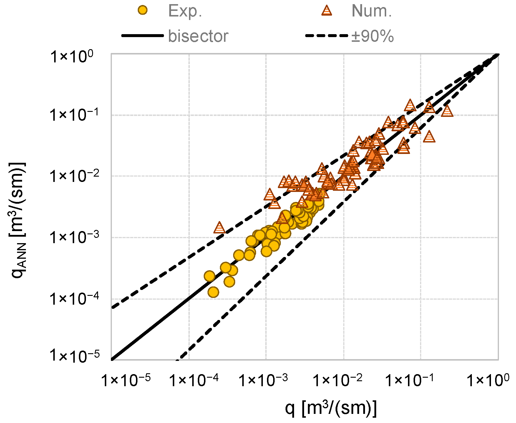
  31. Zanuttigh, B.; Formentin, S.M.; van der Meer, J.W. Advances in modelling wave-structure interaction through Artificial Neural Networks. Coast. Eng. Proc. 2014, 1, 69. [Google Scholar] [CrossRef]
  32. Zanuttigh, B.; Formentin, S.M.; van der Meer, J.W. Prediction of extreme and tolerable wave overtopping discharges through an advanced neural network. Ocean Eng. 2016, 127, 7–22. [Google Scholar] [CrossRef]
  33. Formentin, S.M.; Zanuttigh, B.; van der Meer, J.W. A neural network for predicting wave reflection, overtopping and transmission. Coast. Eng. J. 2017, 59, 1750006. [Google Scholar] [CrossRef]
  34. Zanuttigh, B.; van der Meer, J.W. Wave reflection from coastal structures in design conditions. Coast. Eng. 2008, 55, 771–779. [Google Scholar] [CrossRef]
  35. Muttray, M.; Oumeraci, H.; Ten Oever, E. Wave Reflection and Wave Run-Up at Rubble Mound Breakwaters. Coast. Eng. 2007, 5, 4314–4324. [Google Scholar]
  36. Formentin, S.M.; Zanuttigh, B. A new fully-automatic procedure for the identification and the coupling of the overtopping waves. Coast. Eng. Proc. 2018, 1, 36. [Google Scholar] [CrossRef]
  37. Formentin, S.M.; Zanuttigh, B. Semi-automatic detection of the overtopping waves and reconstruction of the overtopping flow characteristics at coastal structures. Coast. Eng. 2019, 152, 103533. [Google Scholar] [CrossRef]
  38. Lorke, S.; Brüning, A.; Bornschein, A.; Gilli, S.; Krüger, N.; Schüttrumpf, H.; Pohl, R.; Spano, M.; Werk, S. Influence of Wind and Current on Wave Run-Up and Wave Overtopping; Hydralab–FlowDike Report; RWTH Aachen, Institute of Hydraulic Engineering: Aachen, Germany, 2009; p. 100. Available online: http://resolver.tudelft.nl/uuid:73cb6cbe-8931-4499-b4d6-aa31548f5dda (accessed on 22 October 2019).
  39. Lorke, S.; Brüning, A.; Van der Meer, J.; Schüttrumpf, H.; Bornschein, A.; Gilli, S.; Pohl, R.; Spano, M.; Řiha, J.; Werk, S.; et al. On the effect of current on wave run-up and wave overtopping. Coast. Eng. Proc. 2011, 1, 13. [Google Scholar] [CrossRef]
  40. Bijlard, R.; Steendam, G.J.; Verhagen, H.J.; van der Meer, J.W. Determining the critical velocity of grass sods for wave overtopping by a grass pulling device. Coast. Eng. Proc. 2016, 1, 20. [Google Scholar] [CrossRef]
Figure 1. Layout of the numerical flume, including the dike’s cross-section and the position of the wage gauges (wgs), and references to the adopted symbols. Measures in m.
Water 11 02197 g001
Figure 2. Panel (a): scheme of the wave flume and layout of the equipment. Panel (b): cross-sections of the dikes (slopes cot(αoff) = 2 and 4, Gc = 0.15 and 0.3 m) with reference to the position of the ultrasonic velocity profilers (UVPs) along the dike crest (D1, D2 and D3). Measures in m.
Water 11 02197 g002
Figure 3. Experimental and numerical dimensionless values of q as functions of Rc/Hs compared to the curves representing the formulae by EurOtop (2018) for the prediction of q, Equations (1a) and (1b), in panels (a) and (b), respectively. The dashed lines represent the 90% confidence bands associated to the formulae. Data at Rc/Hs ≥ 0 and dry landward conditions.
Water 11 02197 g003
Figure 4. Comparison among experimental and numerical values of q and corresponding predictions from the artificial neural network (ANN). The dashed lines represent the 90% confidence bands associated to the formulae. Data in dry landward conditions.
Water 11 02197 g004
Figure 5. (a) Experimental and numerical values of Kr as functions of ξm−1,0 compared to the curve representing Equation (2) for the prediction of Kr. (b) Comparison among experimental and numerical values of Kr and corresponding predictions from the ANN. The dashed lines represent the 90% confidence bands associated to the formula and the ANN predictions.
Water 11 02197 g005
Figure 6. Layouts of the numerical channel set up for the validation of the code. Structure configuration with Gc = 0.30 and 0.15 m to the top and to the bottom, respectively.
Water 11 02197 g006
Figure 7. Maximum and mean depth (h) envelopes along the dike crest (xc/Gc) as obtained from the image processing (dotted-dashed lines, “video”) and the numerical code (dots, “num”). (Left) Test R00H05s3G30c4; (right) test R10H05s3G30c2.
Water 11 02197 g007
Figure 8. Laboratory (abscissa) and numerical (ordinate) values of h2% (panel (a)) and u2% (panel (b)) calculated at D1 (off-shore edge, diamonds) and D3 (in-shore edge, squares).
Water 11 02197 g008
Figure 9. Comparison among the values of h2% recorded at xc = 0 within the new experimental and numerical tests and literature formulae. The data refer to dry landward conditions and Rc/Hs ≥ 0, are grouped by values of cot(αoff) and are distinguished between experimental (filled in) and numerical (void).
Water 11 02197 g009
Figure 10. Comparison among the values of u2% recorded at xc = 0 within the new experimental and numerical tests and literature formulae. The data refer to dry landward conditions and are grouped by values of cot(αoff) and distinguished between experimental (filled in) and numerical (void). (a) Tests at Rc/Hs > 0; (b) tests at Rc/Hs = 0.
Water 11 02197 g010
Figure 11. Instantaneous vertical profiles (z) of the flow velocity (u) measured at D1 (≈xc = 0) for the test R00H05s3G15c4 in the laboratory (panel (a)) and reproduced with the numerical code (panel (b)). The profiles refer to the instant of occurrence of the maximum flow depth at D1.
Water 11 02197 g011
Figure 12. Comparison among values of u2% at the dike off-shore edge (xc = 0, D1) and average wave celerities c. The data belong to the experimental dataset and are grouped by values of cot(αoff).
Water 11 02197 g012
Figure 13. Frequency distribution of the values of u measured at D1 (≈xc = 0) for the same experimental test H05s3G30c4, conducted at zero (R00) and in emerged freeboard (R10) conditions. The flow is in-shore and off-shore directed when the values of u are, respectively, >0 and <0.
Water 11 02197 g013
Figure 14. Comparison among the values of h2% recorded at xc = 0 during the new tests (a) and the FlowDike data experiments (b) and the new fitting by Equation (5). The data are grouped by values of cot(αoff).
Water 11 02197 g014
Figure 15. Comparison among the values of u2% recorded at xc = 0 during the new tests (a) and the FlowDike data experiments (b) and the new fitting by Equation (6). The data are grouped by values of cot(αoff) and relate to Rc > 0 only.
Water 11 02197 g015
Figure 16. Evolution of the flow thickness (h2%/h2%,xc = 0, panel (a)) and of the flow velocity (u2%/u2%,xc = 0, panel (b)) along the dike crest (xc/Gc). Average values from the numerical tests grouped by Rc/Hs.
Water 11 02197 g016
Figure 17. Frames of an overtopping event propagating over the dike crest during the same test R00H05s3G30c4, relative to a breaking wave, and carried out in the laboratory (a) and by the numerical code (b). The color map displays the computational field of the u-velocity (m/s).
Water 11 02197 g017
Figure 18. Consecutive frames of an overtopping event propagating over the dike crest during a numerical (a) and an experimental (b) test (R00H05s2G30c2) relative to non-breaking wave conditions. The color map of panel (a) displays the u-velocity field (m/s).
Water 11 02197 g018
Figure 19. Comparison among values of u2% measured at the off-shore (xc = 0) and in-shore (xc = Gc) edges of the dike crest in the lab experiments (a) and the numerical simulations (b). The data are grouped by values of cot(αoff). All the tests are at Rc/Hs ≥ 0.
Water 11 02197 g019
Figure 20. Frequency distribution of the instantaneous depth-averaged values of u at the dike off-shore (blu) and in-shore (orange) edges for the same experimental test (H05s3G30c4) at Rc/Hs = 0 (panel (a)) and Rc/Hs > 0 (panel (b)).
Water 11 02197 g020
Figure 21. Comparison among values of u2%(xc = 0) to corresponding values of u2%(xc = Gc) for wet (a) and dry (b) landward conditions. The data belong to the numerical database and are grouped by values of Rc/Hs. For all the data, Rc/Hs < 0.
Water 11 02197 g021
Table 1. Synthesis of the range of configurations tested in the numerical model. The “dry” landward conditions were carried out with Hs = 0.2 m and Hs/Lm−1,0,t = 0.02 and 0.03 only.
Rc/Hs−1.5−1−0.5−0.20+0.5+1+1.5
Hs/Lm−1,0,t0.02; 0.030.02; 0.03; 0.040.02; 0.03; 0.050.020.02; 0.03; 0.04; 0.050.02; 0.03; 0.040.02; 0.03; 0.050.03
Hs (m)0.1; 0.20.1; 0.20.1; 0.20.20.1; 0.20.1; 0.20.20.2
cot(αoff)4; 64; 64; 64; 64; 64; 64; 64; 6
cot(αin)33333333
Landwardwet; drywet; drywet; drydrywet; drywet; drydrydry
Table 2. Summary of the target conditions of the 60 experiments of wave overtopping at dikes performed in the Laboratory of Bologna.
Rc/Hs0+0.5+1
sm−1,0 (%)3; 43; 43; 4
Hs (m)0.04; 0.05; 0.060.04; 0.05; 0.060.05; 0.06
wd (m)0.35[0.32; 0.325][0.29; 0.30]
cot(αoff)2; 42; 42; 4
Gc (m)0.15; 0.300.15; 0.300.15; 0.30
Landwarddrydrydry
Tot. #241818
Table 3. Error indexes R2 and σ% characterizing the agreement between the new laboratory/numerical data of q and Kr and corresponding predictions from literature methods.
qKr
DatasetEquations (1a)–(1b)ANNEquation (2)ANN
σ%R2σ%R2σ%R2σ%R2
Laboratory56%0.8712%0.9145%0.7740%0.89
Numerical16%0.9527%0.8128%0.906.0%0.93
Table 4. Summary of the 12 experimental tests carried out at the Laboratory of Bologna and reproduced in the numerical code.
Test IDHm0
(m)
Tm−1,0
(s)
Rc/Hs
(-)
cotα
(-)
Gc
(m)
ξm−1,0
(-)
q/(gHsTm−1,0)
(-)
Kr
(-)
LabNumLabNum---LabNumLabNumLabNum
R00H05s3G15c40.0470.0421.0481.0830.0040.151.521.687.80 × 10−37.6 × 10−30.160.20
R00H05s3G15c20.0490.0491.0361.0400.0020.152.932.937.09 × 10−31.8 × 10−30.370.41
R00H05s3G30c40.0460.0421.0481.1900.0040.301.521.817.02 × 10−37.5 × 10−30.170.18
R00H05s3G30c20.0480.0481.0361.1900.0020.32.943.407.48 × 10−38.0 × 10−30.320.36
R05H05s3G15c40.0530.0441.0761.1050.5040.151.461.642.54 × 10−32.5 × 10−30.340.26
R05H05s3G15c20.0530.0461.3741.1050.5020.153.723.222.49 × 10−32.7 × 10−30.530.48
R05H05s3G30c40.0480.0441.0761.1050.5040.301.531.642.49 × 10−32.4 × 10−30.280.26
R05H05s3G30c20.0540.0481.0521.1050.5020.32.553.153.22 × 10−32.4 × 10−30.530.51
R10H05s3G15c40.0560.0421.1.0401.0040.151.371.598.02 × 10−49.3× 10−40.410.27
R10H05s3G15c20.0570.0451.0081.0401.0020.152.643.061.43 × 10−31.1 × 10−30.620.57
R10H05s3G30c40.0490.0421.0361.0401.0040.301.461.596.87× 10−49.7× 10−40.290.27
R10H05s3G30c20.0570.0461.0081.0401.0020.32.633.041.50 × 10−31.1 × 10−30.630.58
μ (Num/Lab)0.871.02---1.110.940.96
σ% (Num/Lab)8.0%8.4%---9.7%28%16%
Table 5. Values of the coefficients ch and cu adopted by the several authors in the formulae for the evaluation of h2% and u2% based on the scheme of Equations (4) and (5).
Author(s)Flow CharacteristicCoefficientAdopted Value/FormulationValidity Range
Schüttrumpf (2001) [4]h2%(xc = 0)ch0.33cot(αoff) = 3, 4 and 6; Rc ≥ 0
u2%(xc = 0)
(flow velocity)
cu1.37
Van Gent (2002)
[5]
h2%(xc = 0)ch0.15cot(αoff) = 4; Rc > 0
u2%(xc = 0)
(flow velocity)
cu1.33
Bosman et al. (2008)
[8]
h2%(xc = 0)ch0.01/sin2(αoff),
for cot(αoff) = 4 or 6
cot(αoff) = 4 and 6; Rc > 0
u2%(xc = 0)
(wave celerity)
cu0.30/sin(αoff),
for cot(αoff) = 4 or 6
Van der Meer et al. (2010) [1]u2%(xc = 0)
(wave celerity)
cu0.35∙cot(αoff),
for cot(αoff) = 4 or 6
cot(αoff) = 3, 4 and 6; Rc ≥ 0
Table 6. Error indexes R2 and σ% characterizing the agreement between the data of h2%(xc = 0) and u2%(xc = 0) and the new fitting by Equations (5) and (6).
Dataseth2%(xc = 0)-Equation (5)u2%(xc = 0)-Equation (6)h2%(xc = 0)-Equation (3), [8]u2%(xc = 0)-Equation (4), [8]
σ%R2σ%R2σ%R2σ%R2
New laboratory data 41%0.8215.2%0.8237.2%-24.8%-
New numerical data4.1%0.9922.1%0.7341.9%-71.9%-
FlowDike1 data—c343.4%0.8541.8%0.7942.7%0.8543.2%0.77
FlowDike2 data—c642.3%0.8450.7%0.8843.8%0.6769.9%0.85

