Effects of Submerged Vegetation Density on Turbulent Flow Characteristics in an Open Channel

Abstract

The vegetation density λ affects turbulent flow type in the submerged vegetated river. This laboratory study investigates different types of vegetated turbulent flow, especially the flow at 0.04 < λ < 0.1 and λ = 1.44 by setting the experimental λ within a large range. Vertical distributions of turbulent statistics (velocity, shear stress and skewness coefficients), turbulence kinetic generation rate and turbulence spectra in different λ conditions have been presented and compared. Results indicate that for flow at 0.04 < λ < 0.1, the profiles of turbulent statistics manifest characteristics that are similar to those of both the bed-shear flow and the free-shear flow, and the turbulence spectral curves are characterized with some slight humps within the low-frequency range. For λ = 1.44, the turbulent statistics above the vegetation top demonstrate the characteristics of boundary-shear flow. The spectral curves fluctuate intensely within the low-frequency range, and the spectra of low-frequency eddies above vegetation top are significantly larger than the values below. The change of turbulent flow type induced by an increase of λ would increase the maximum value of turbulence kinetic generation rate G_S and change the point where G_S is vertically maximum upwards to the vegetation top.

1. Introduction

Aquatic vegetation is ubiquitous in rivers, which affects the sediment transport, scalar dispersion, channel evolution and aquatic biodiversity by interfering with the flow field [1,2,3,4]. The investigation of vegetated flow can lead to a better understanding on fluvial process and hydro-environment prospect of vegetated rivers.

In an open channel with submerged vegetation, the turbulent flow type in the longitudinal- vertical (x–z) plane varies with an increase of vegetation density, from the bed-shear flow to the free-shear flow and the secondary boundary-shear flow [5,6]. The bed-shear flow happens because of bed drag near the flume bottom, with vegetation contributing to the bed roughness and increasing the bed friction [5]. For the medium dense vegetation, flow discontinuity caused by canopy drag would occur at the vegetation top, generating the free-shear flow in certain vertical region. Yan et al. [7] assumed that in extremely dense vegetation condition, flow was nearly static within canopy and flow characteristics above canopy were similar to the ones in bed-shear flow [6]. Flow in this extremely dense vegetation condition is named as the secondary boundary-shear flow with the “boundary” locating at canopy top [6].

Vegetation density λ can be defined as the frontal vegetation area per unit bed area. Nepf [5] proposed that the bed-shear flow and free-shear flow occur at 0 < λ < 0.04 and 0.1 < λ < λ_NB, respectively. Here, λ_NB is the critical density which indicates the change from the free-shear flow to the secondary boundary-shear flow. The value of λ_NB has not been determined yet, but according to the comparison and summary of many investigations, λ_NB might lie in the range between 0.512 and 1.55 [6].

Previous studies have investigated the bed-shear flow (0 < λ < 0.04) and the free-shear flow (0.1 < λ < λ_NB), especially the latter one in the vegetated channel. Flow at 0.04 < λ < 0.1 and λ > λ_NB (the secondary boundary-shear flow may appear) have been rarely analyzed. In the present investigation, flow characteristics have been measured and analyzed as λ varies within a large range. Based on vertical distributions of turbulent statistics (velocity, shear stress, skewness coefficients), turbulence kinetic generation rate and turbulence spectra, different flow types have been verified. Furthermore, flow characteristics and velocity distribution laws at 0.04 < λ < 0.1 and λ > λ_NB are discussed specifically.

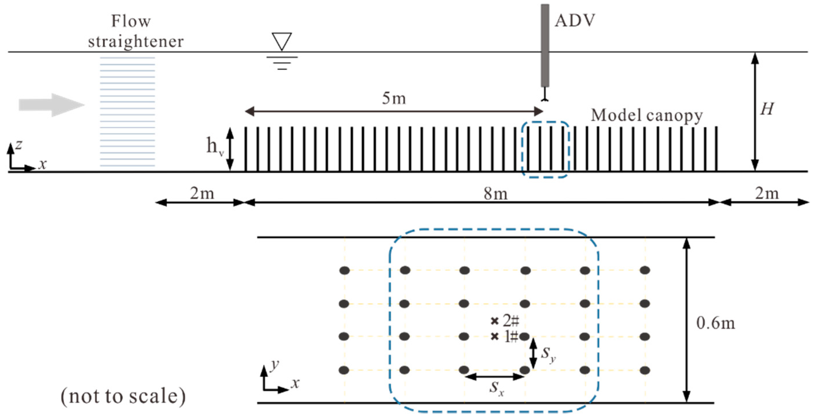
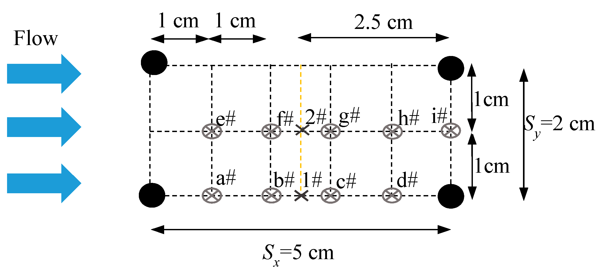
2. Experimental Setup and Measurement

Laboratory experiments were conducted in a 12-m-long, 60-cm-wide (B = 60 cm), 60-cm-deep recirculating flume (Figure 1). An ultrasonic flow meter (Krohne, Germany) with an accuracy of 0.001 L/s was used to monitor flow discharge Q, which was maintained constant by a variable frequency pump system. The flow from the water tank passed through a flow-straightener upstream of the vegetation section to smooth the inflow. A tailgate was mounted at the outlet of the flume to control the flow depth H in the experiment. The bed slope was adjustable to create longitudinally uniform flow, which was judged according to the flow depths measured along the streamwise direction. Flow depth was measured by rulers with an accuracy of 0.5 mm placed on the glass sidewall at a spacing of 1 m.

Vegetation was simulated by 6-cm-high (i.e., h_v = 6 cm) aluminum cylinder with diameter d_v = 0.6 cm. In order to place the cylinders in the channel bed, an artificial bottom was constructed with an 8-m-long plate of 0.6-cm-holed pegboard. The streamwise and spanwise spacings between neighboring cylinders were defined as S_x and S_y respectively. The vegetation was linearly arranged at the mid 8 m length of the flume, and λ was calculated by λ = (d_v h_v)/(S_x S_y).

3D flow velocity was measured by an acoustic Doppler velocimeters (ADV, Nortek, Norway) with an accuracy of ±1 mm/s, mounted on an automatic traversing system that could move in three orthogonal directions with a step of 0.1 mm. The sampling period was set to be 180 seconds with a frequency of 200 Hz. The device with four probes had a 5-cm blind zone near the water surface for velocity measurement, which was, therefore, supplemented by another device with lateral probes.

Velocity profiles were measured at the section 5 m downstream of the leading edge of the canopy area, where the flow was fully developed in the longitudinal direction. Velocities at two locations (shown as locations 1# and 2# in Figure 1) in the test area were measured and averaged to represent the overall flow.

Flow measurements were started at z = 1 mm at intervals of Δz = 2 mm moving upwards to the free surface. As the stems did not allow the access of ADV probes, velocities within 2.1 cm above the channel bed at location 1# could not be measured. Flow in this region is characterized with wake turbulence that changes little with the cylinders heights. Therefore, this measurement limitation was overcome by replacing two obstructive cylinders of 6cm height with cylinders of 4 cm height.

This experimental investigation is mainly to investigate the influence of λ; therefore, we maintained the flow depth H and the flow discharge Q constant for different cases. Hence, the relative submergence Sub = H/h_v and the mean bulk velocity U_m = Q/(BH) remain constant in the experiment. The flow with Sub = 3 and U_m = 30 cm/s in this study represented the high-speed shallow flow. The experimental λ was selected from a wide range to create different flow conditions. According to [5], the bed-shear flow and free-shear flow may occur in Cases I & II (λ = 0, 0.0056) and Case V (λ = 0.36), respectively (

Table 1. Experimental conditions.

Case	λ	Sx (cm)	Sy (cm)	H (cm)	Sub	Q (L/s)	Um (cm/s)
I	0	0	0	18	—	32.44	30.04
II	0.0056	40	16	18	3	32.34	29.94
III	0.045	10	8	18	3	32.43	30.03
IV	0.09	5	8	18	3	32.35	29.95
V	0.36	5	2	18	3	32.4	30
VI	1.44	2.5	1	18	3	32.48	30.07

).

Velocity profiles at another 9 locations (from location a# to location i# in Figure 2) in flow field for Case V were measured additionally to study spatial variations of the flow characteristics and the representative locations of the canopy flow. The 9 locations were distributed evenly and fully within the bed area of S_x × S_y It is, thus, believed the spatial averages of the experimental data at these 9 locations can represent the overall flow. A comparison between the averaged velocity at the 9 locations and the averaged velocity at points 1# and 2# was conducted to verify that the measurements for points 1# & 2# are indeed representative.

3. Results

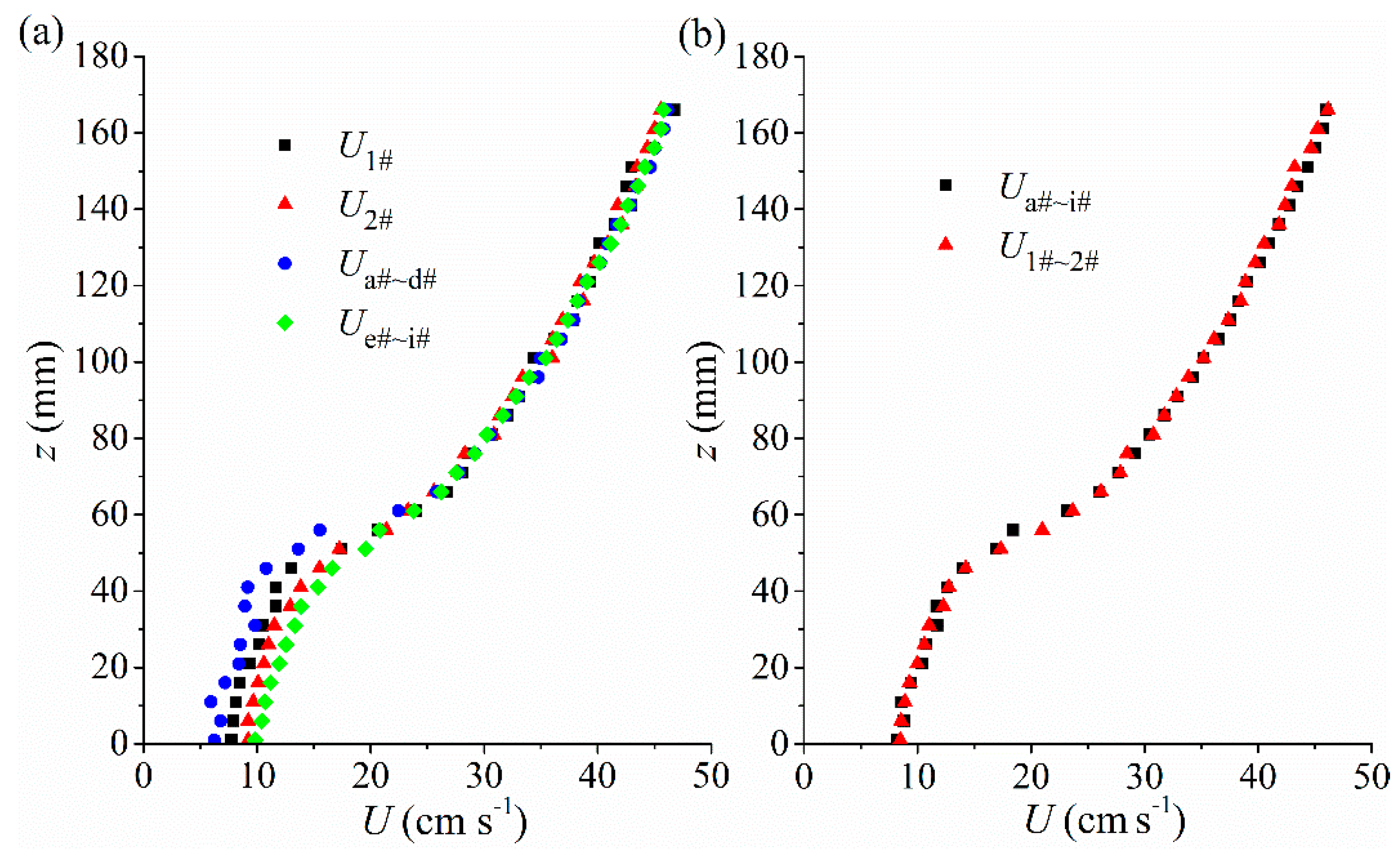
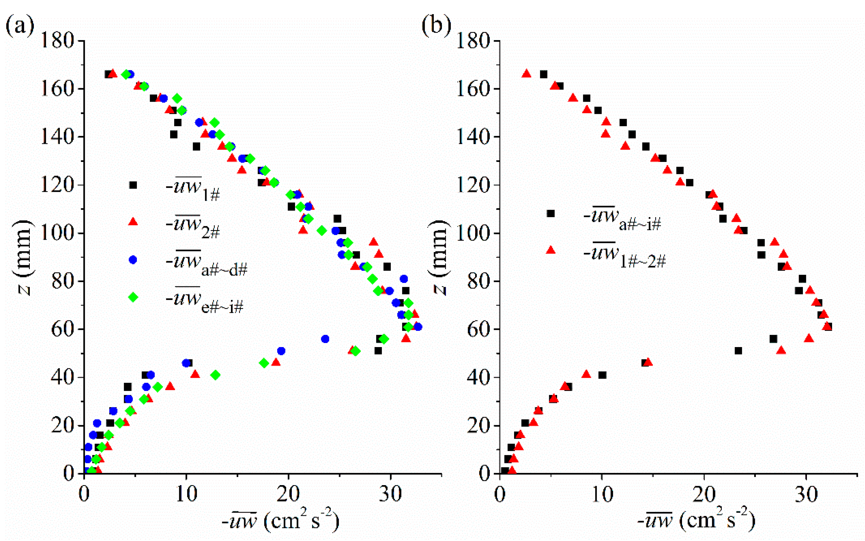
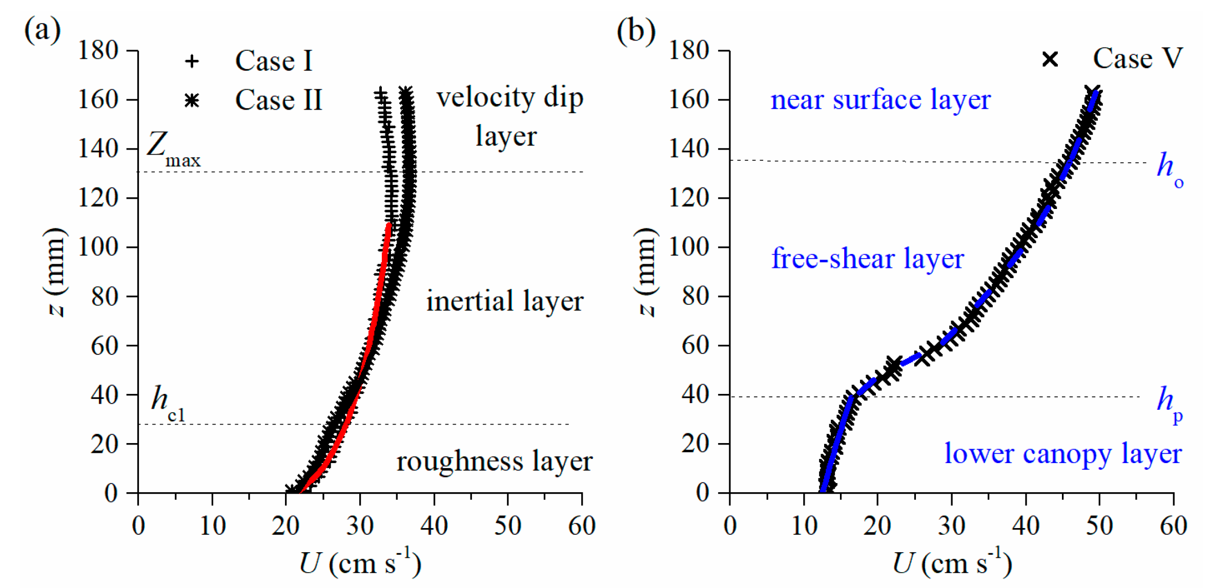
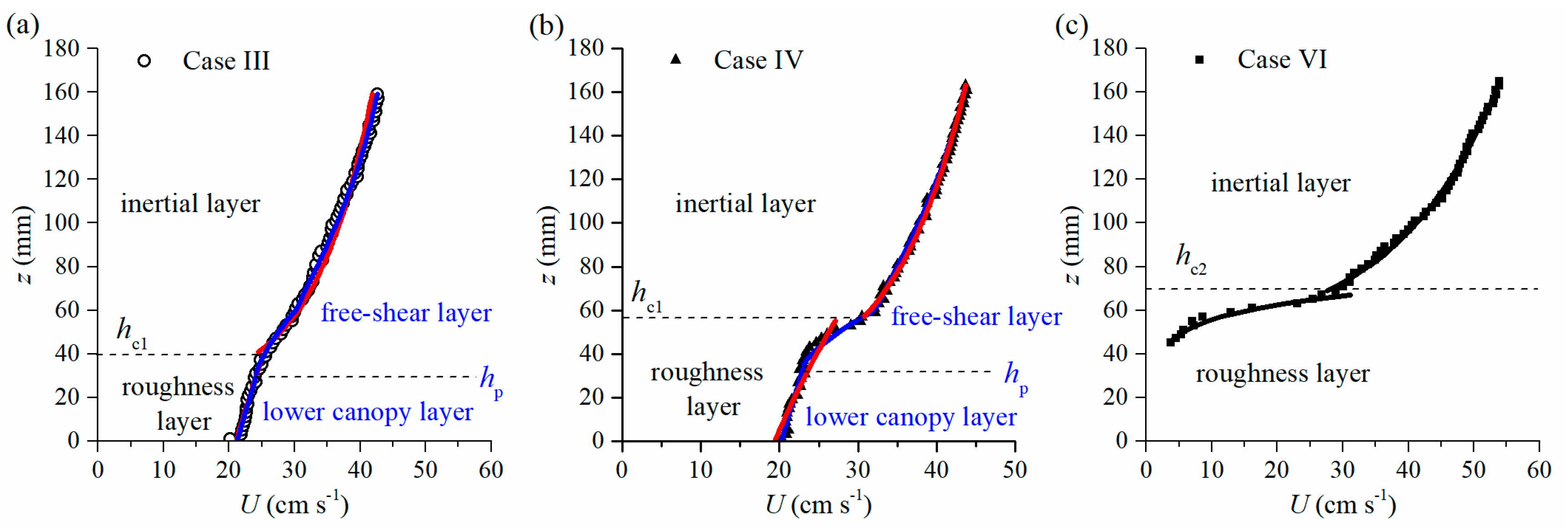
3.1. Spatial Variation of the Velocity and Reynolds Stress Profiles

Figure 3 and Figure 4 compare the velocity profiles and the Reynolds stress distributions at different locations for Case V. The values characterized with subscripts of “a#~i#”, “1#~2#”, “a#~d#” and “e#~i#” denote the space-averaged values from location a# to i#, 1# to 2#, a# to d# and e# to i#, respectively. Therefore, U_a#~i# and $-{\overline{uw}}_{a\#~i\#}$ represent the overall space-averaged flow characteristics in the experiment.

The velocity U and Reynolds shear stress $-\overline{uw}$ (u and w denote velocity fluctuations in the x and z directions, respectively) vary horizontally in canopy layer meanwhile the profiles for different locations concentrate above the canopy (Figure 3a and Figure 4a). The flow shear in the free stream (Locations e#~ i# & 2#) with larger U and $-\overline{uw}$ is comparatively intensive than that behind the vegetation (Locations a#~ d# & 1#). The results that U_1# > U_a#~d#, U_2# < U_e#~i# and U_1# < U_2# are shown in Figure 3a. However, $-{\overline{uw}}_{1\#}\approx -{\overline{uw}}_{a\#~d\#}$, $-{\overline{uw}}_{2\#}\approx -{\overline{uw}}_{e\#~i\#}$ and $-{\overline{uw}}_{1\#}<-{\overline{uw}}_{2\#}$ are shown in Figure 4a.

Figure 3b and Figure 4b show that U_1#~2# ≈ U_a#~i# and $-{\overline{uw}}_{1\#~2\#}\approx -{\overline{uw}}_{a\#~i\#}$, respectively, throughout the depth. Hence, it is sufficiently accurate to describe the overall flow dynamics by the averaged velocity of points 1# and 2#. In this study, therefore, we analyze the flow characteristics by the averaged values of points 1# and 2#. The subscript is omitted in the rest sections of this article.

3.2. Turbulent Statistics

3.2.1. Velocity

Figure 5 presents the velocity profiles for different λ, and the averaged velocity gradients dU/dz in specific regions have been listed in

Table 2. The velocity gradient dU/dz (s⁻¹) in different regions.

	Case I	Case II	Case III	Case IV	Case V	Case VI
0 < z< 10 mm	2.99	3.462	2.407	2.03	−0.068	—
55 ≤ z ≤ 65 mm	1.126	1.38	2.025	3.077	4.978	19.764

— indicates that the value is not available because the flow field near the bed cannot be measured.

. In order to show each profile clearly, the profiles are plotted in two pictures. The vertical regions where U increase considerably are marked with red curves in Figure 5.

The velocity U increases considerably near the channel bed (0 < z < 10 mm) for Cases I & II (Figure 5a & Table 2), which shows the characteristics of the bed-shear flow [8], and dU/dz = 3 s⁻¹ in this region. For Case V, U increases rapidly near the canopy top (55 ≤ z ≤ 65 mm) and dU/dz = 5 s⁻¹ there (Figure 5b & Table 2), which indicates intensive shear exists in this region under this flow condition.

For Cases III & IV which 0.04 < λ < 0.1, the velocity U increases considerably both near the bed and at the canopy top (Figure 5a & Table 2). dU/dz vary from 2 to 2.4 s⁻¹ near the channel bed and 2 to 3 s⁻¹ around the vegetation top, which are between the ones for Cases I & II (bed-shear flow) and the one for Case V (free-shear flow) (Table 2).

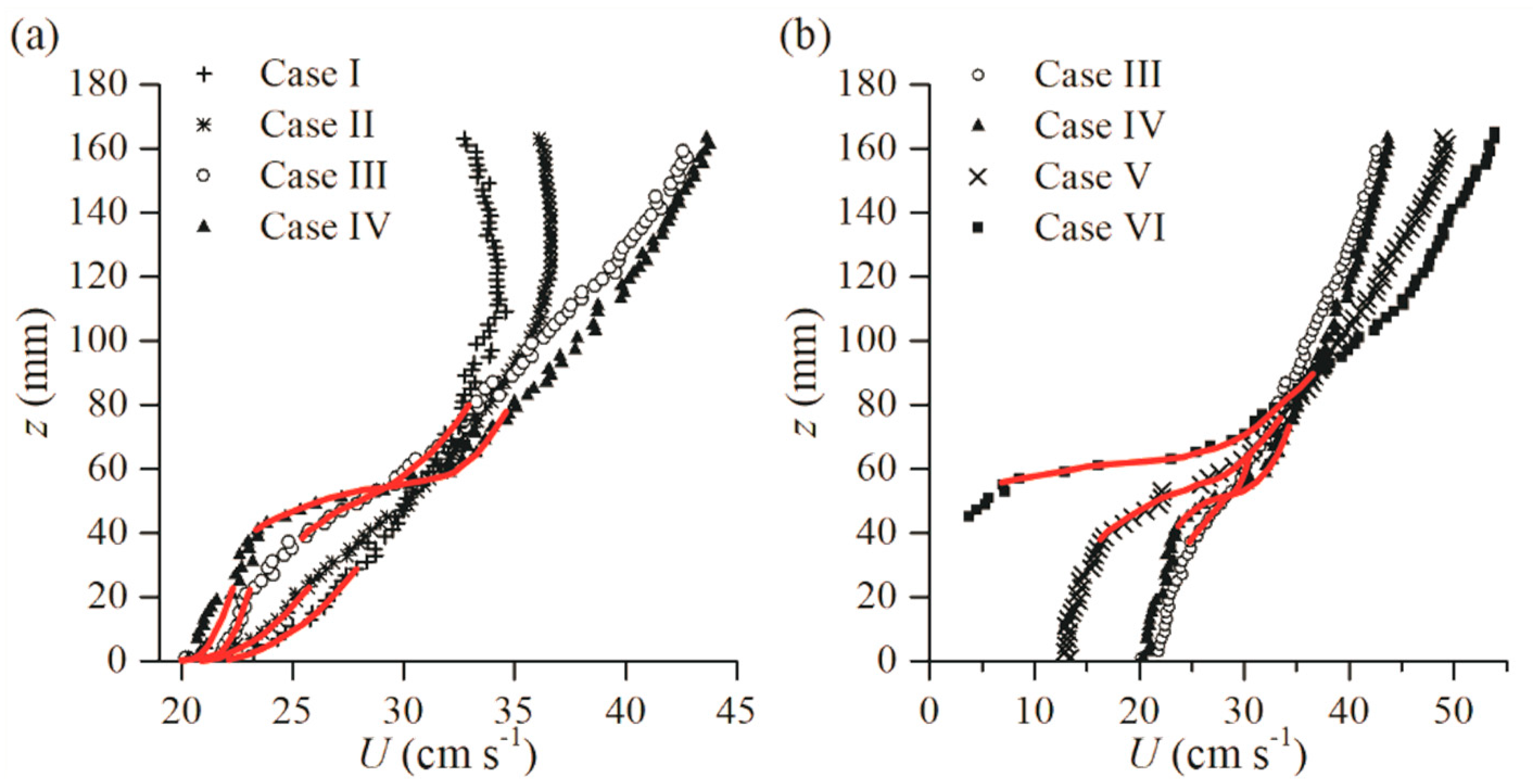
In Case VI, the velocity profile along the water depth is highly similar to the one presented in [9] with λ = 1.544 and increases sharply above the canopy but is small within the canopy (Figure 5b). dU/dz around the canopy top is far greater than those of other cases. That indicates intensive stress appears at the canopy top, and the canopy top can be considered as a “new bed” at this density.

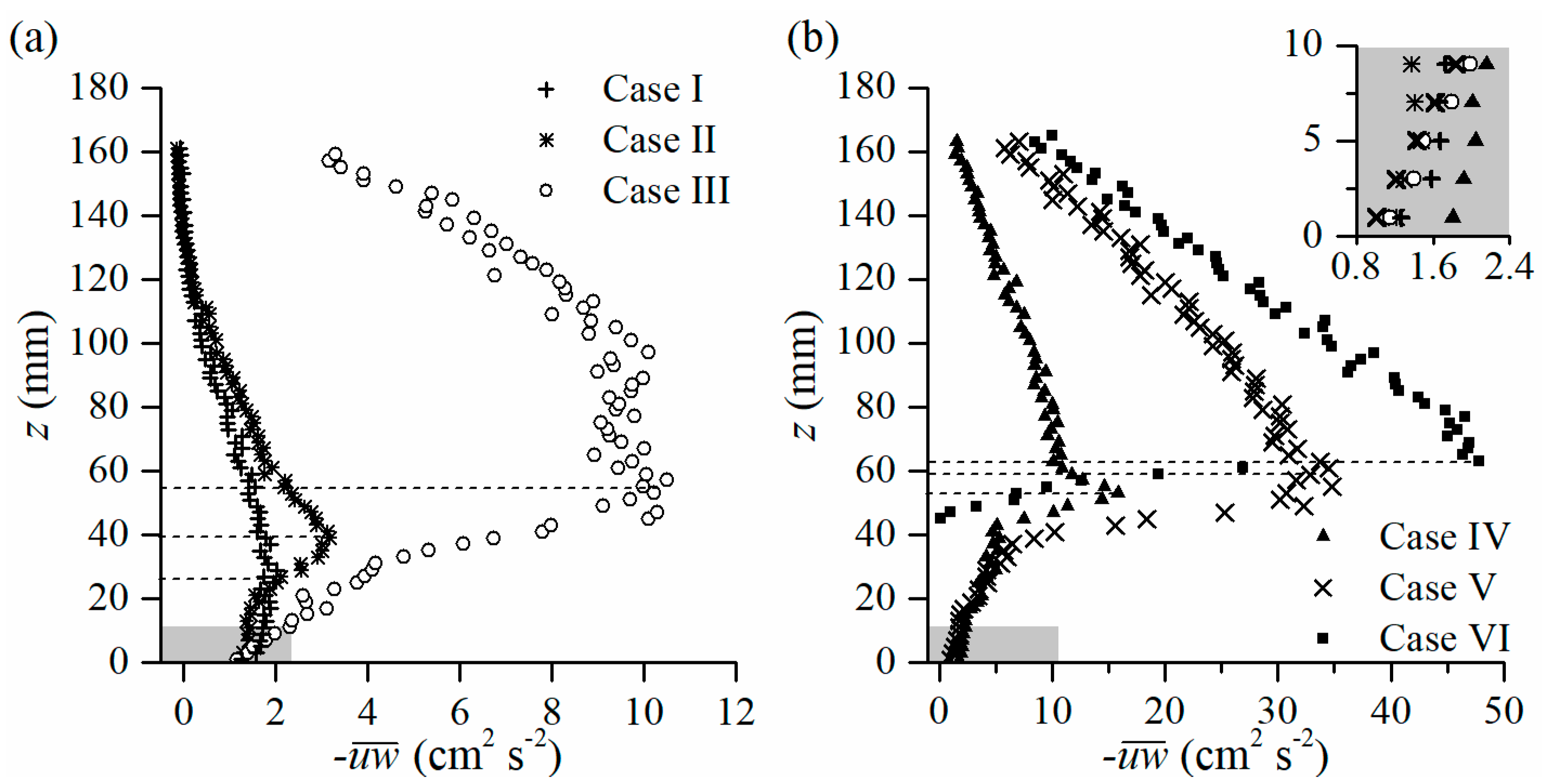
3.2.2. Shear Stress

The Reynolds shear stress $-\overline{uw}$ increases along z in a certain region near the bed and then decreases towards the free surface for all the cases (Figure 6). For Cases I & II (bed-shear flow), the shear stress $-\overline{uw}$ attains its peak at z = (0.15~0.2) H (Figure 6a), which is the upper boundary of the inner region [7]. The height of the $-\overline{uw}$ peak for Case II (with vegetation) is higher than the one for Case I (with no vegetation) (Figure 6a). In Case V, the peak of $-\overline{uw}$ appears at the canopy level z = h_v (Figure 6b) and the free-shear flow happens because of flow discontinuity at the canopy top [10].

The $-\overline{uw}$ profile in Case VI is similar to the one in Case V, except that the $-\overline{uw}$ is nearly zero within canopy. In Cases III & IV, the maximum $-\overline{uw}$ appears between the one for Cases I & II (bed-shear flow) and the one for Case V (free-shear flow) in Figure 6.

In the region near the bed, the largest $-\overline{uw}$ appears in Case IV (λ = 0.09) comparing with other cases (see the partially enlarged figure in Figure 6b). Although the difference is small among the 6 cases, the result could yet be applied to explain why the flow velocity for sediment incipient motion is minimum or the bed load transport rate is maximum while λ varies around 0.09 [11,12].

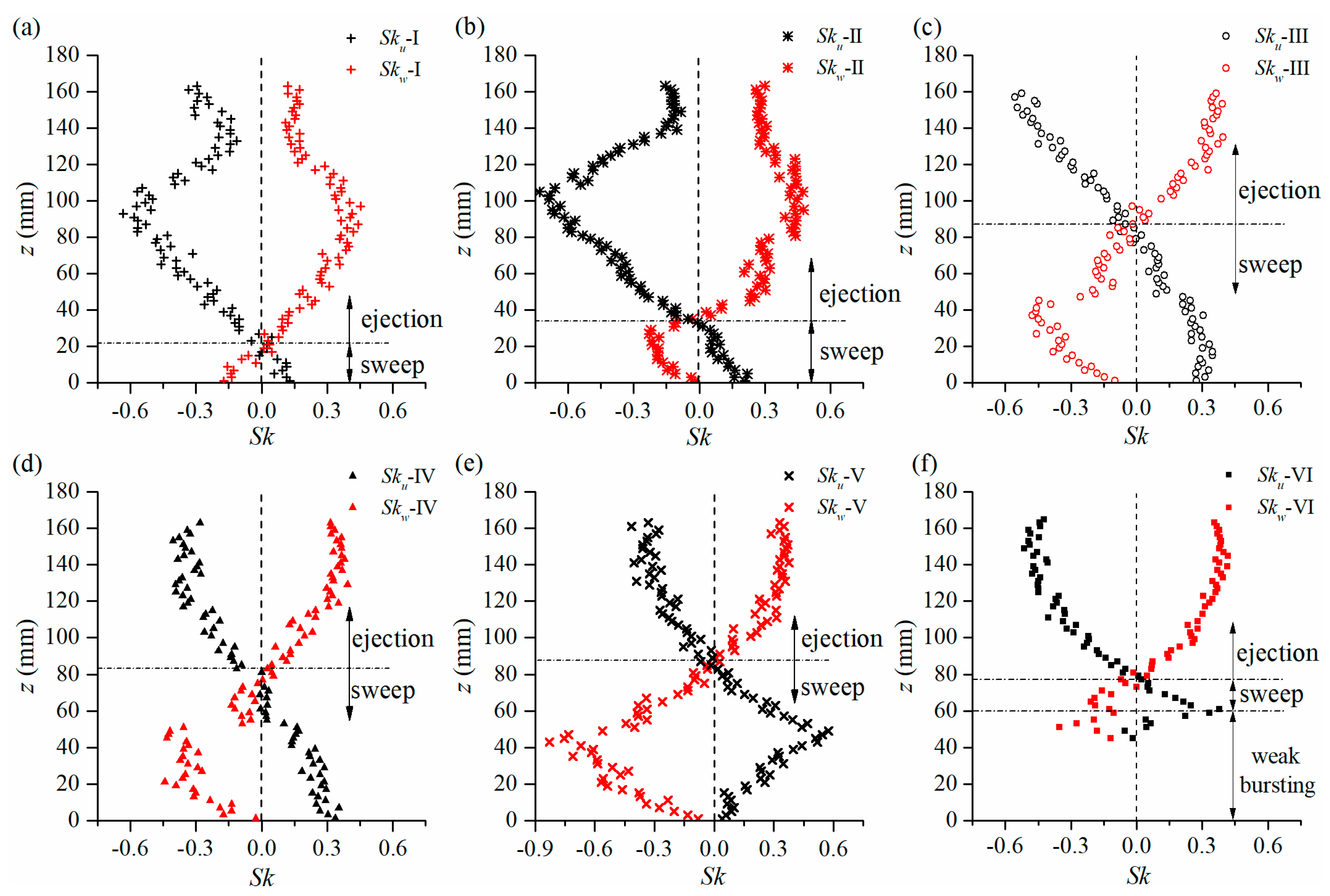
3.2.3. Skewness Coefficients

Turbulence affects bursting events along the depth, and the bursting phenomenon could be judged according to the skewness coefficients [9]. The skewness coefficients are defined as:

$$S{k}_u=\frac{1}{N}{\displaystyle \sum _{i=1}^N{u}^3}/{\left(\sqrt{\frac{1}{N}{\displaystyle \sum _{i=1}^N{u}^2}}\right)}^3$$

(1)

$$S{k}_w=\frac{1}{N}{\displaystyle \sum _{i=1}^N{w}^3}/{\left(\sqrt{\frac{1}{N}{\displaystyle \sum _{i=1}^N{w}^2}}\right)}^3$$

(2)

where N is the sampling number, Sk_u and Sk_w are the skewness coefficients of u and w, respectively. Bursting phenomenon manifests in four different manners, i.e., outward interaction (Sk_u > 0, Sk_w > 0), ejection (Sk_u < 0, Sk_w > 0), inward interaction (Sk_u < 0, Sk_w < 0) and sweep (Sk_u > 0, Sk_w < 0) [8]. The absolute values of Sk_u and Sk_w reflect the intensity degree of the bursting actions [13].

Sweep occurs in the lower flow zone while ejection appears in the upper zone for all the experiment cases (Figure 7).

For Cases I & II (Figure 7a,b), the sweep is the most intensive at the flume bed. The ejection achieves the utmost at the mid flow depth (z = 93 mm in Case I and 105 mm in Case II), which is caused by the sidewall effect in a narrow channel [13]. The strongest sweep appears at z = 45 mm, while the ejection is the fiercest at the water surface for Case V (Figure 7e).

When it comes to Case VI, the Sk_u and Sk_w profiles above canopy (Figure 7f) are similar to those throughout depth in the bed-shear flow. Meanwhile, the ejection action is vertically fiercest near the free surface (Figure 7f), indicating that the sidewall effect disappears in Case VI.

The bursting events for Cases III & IV manifest the characteristics of both the free-shear flow and bed-shear flow (Figure 7c,d): Sk_w profiles are similar to the one for the free-shear flow; however, Sk_u attains its vertical maximum at the bottom, which is in line with that for the bed-shear flow.

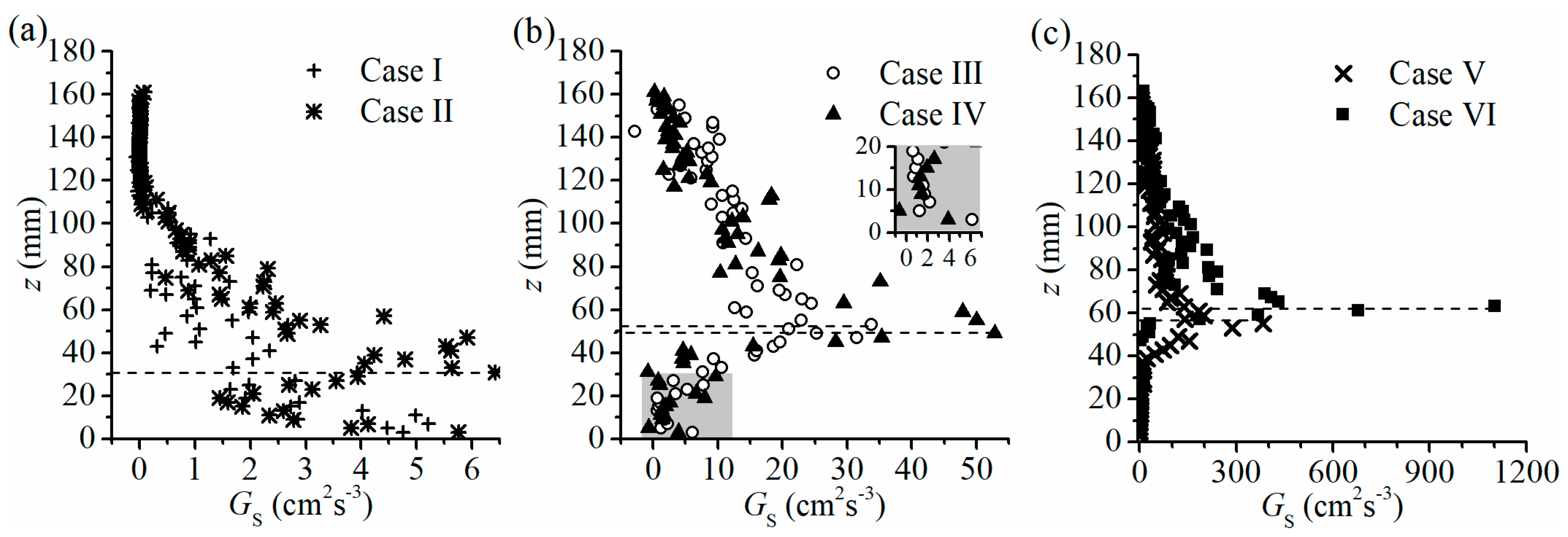
3.3. Turbulence Kinetic Energy Generation Rate

The turbulence kinetic energy generation rate G_S, $G_S=-\overline{uw}\frac{\partial U}{\partial z}$, represents the turbulent energy that is drained from the mean flow. We compute G_S by the measured data and plot G_S profiles corresponding to different vegetation densities in Figure 8.

For Case I (bed-shear flow with no vegetation), G_S decreases with z and its vertical maximum appears at the channel bottom. However, for Case II (the bed-shear flow with sparse vegetation), G_S attains its peak both at the flume bottom and at a certain height above the bed (z = 31 mm). Meanwhile, G_S in Case II is larger than that in Case I.

In Cases III & IV, the height of vertical maximum G_S is slightly below the vegetation top (Figure 8b). G_S within canopy decreases towards the bed but increases suddenly on the bed (see the partially enlarged figure in Figure 8b). The near bed G_S values approximate the ones in Cases I & II.

The maximum of G_S is increasing continuously from Cases I & II, Case III & IV, Case V to Case VI (Figure 8), indicating that the change of the turbulent flow type, which is induced by an increase of λ, would intensify the flow turbulence.

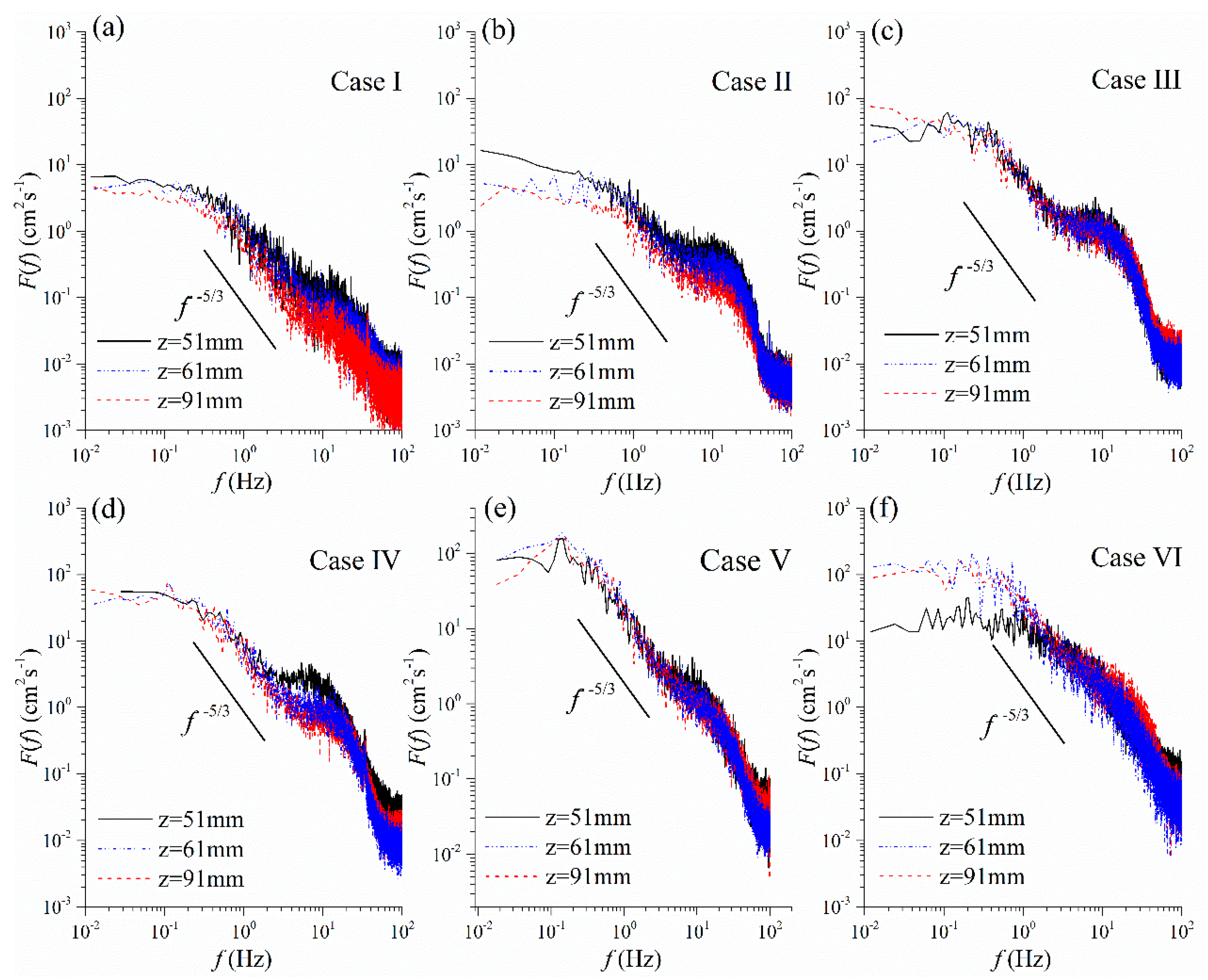
3.4. Turbulence Spectra

The turbulence spectra F(f) represents the turbulence kinetic energy of eddies with different frequencies f. Basing on the Taylor’s frozen hypothesis, the F(f) ~ f relation could be obtained by the Fourier Transformation of the velocity series at any point. The maximum time lag was set at 23% of the time series length in this study.

Figure 9 presents the spectra of longitudinal velocities along the vertical direction. For turbulence around the vegetation top the spectral densities increase with λ in Figure 9, which coincides with the influence of λ on the maximum G_S among different cases (Figure 8). The intermediate frequency in this study except z = 51 mm in Case VI ranges from 0.4 to 4 Hz where the −5/3 power law is satisfied, which is characteristic of the systematic cascade of turbulence energy within the inertial subrange (ISR).

In the low-frequency range below ISR, the spectral curves vary along the vertical, and the change tendency is affected by the turbulent flow type. For the bed-shear flow in Cases I & II, especially the one at z = 51 or 91 mm, F(f) tends to decrease slightly with f, which coincides with the one presented in an open channel with no vegetation [14]. The low frequency eddies would evolve upwards towards the free surface, so that the corresponding F(f) decreases from z = 51 mm to z= 61 and 91 mm in Figure 9a,b. For the free-shear flow in Case V, the spectral curve peaks at 0.15 Hz and the peak frequency does not change with vertical height (Figure 9e), as mentioned by [15] in a study of the free-shear flow. The spectral curve is the highest at z = 61 mm (i.e., the vegetation top) because the flow shears intensely there.

For Cases III & IV at 0.04 < λ < 0.1, there are some slight spectral humps whose frequencies vary around 0.15 Hz. The peak spectra in these conditions are smaller than the one in the free-shear flow because of the relatively weak turbulence caused by discontinuity in flow resistance. The F(f) changes little with the gauging height in Figure 9c,d.

For Case VI, the spectral curve fluctuates intensely within the low-frequency range. The curve at z = 61 mm nearly coincides with the one at z = 91 mm and is higher than the one at z = 51 mm. The height of z = 51 mm locates within the canopy, where the low speed porous media flow might happen in this dense vegetation condition with λ = 1.44.

3.5. Distribution Law of the Velocity Profiles

For bed-shear turbulent flow, the U profile is logarithmic in a certain vertical region (i.e., the inertial layer) [16]. We define the lower boundary height of the inertial layer as h_c1 where the U profile deviates from the logarithmic law toward the bed. Figure 10a shows that the inertial layer starts from the channel bed (i.e., h_c1 = 0), when there is no-vegetation (Case I, the red line); while it locates above the bed (i.e., h_c1 > 0) in case of a sparsely vegetated condition (Case II, the black line). For the roughness layer (0 < z < h_c1) below in Case II, the exponential function [17] has been adopted to fit the measured U data, which leads to the coefficients of determination R² = 0.9229.

In Figure 10a, maximum U appears below the free surface because of the sidewall effect in the cross-section, which means velocity dip phenomenon. This phenomenon had been observed in a narrow open channel flow [14] and in the vegetated flow [18]. We define the height of the maximum velocity as Z_max and the region from z = Z_max to the free surface as the velocity dip layer, respectively. The U profile in the velocity dip layer could be described by a power law, with R² = 0.9015 for Case II (Figure 10a).

Case V is characterized with the free-shear flow, which could be divided into three layers as the lower canopy layer (0 < z < h_p), the intermediate free-shear layer (h_p < z< h_o) and the surface layer (h_o < z < H) [9]. h_p and h_o are the boundaries of the free-shear layer that could be estimated by the displacement height and the turbulent kinetic energy balance, respectively [19,20]. Experimental U data in the free-shear layer and the surface layer were fitted by the hyperbolic tangent function with R² = 0.9986 and logarithmic function with R² = 0.986 (see the blue dash line in Figure 10b), respectively. The U data in the lower canopy layer was compared with the power, exponential and logarithmic functions, of previous studies [17,18,21], separately. An exponential distribution law is satisfied in this region with R² = 0.9328 (see Figure 10b).

For flow at 0.04 < λ < 0.1, i.e., Cases III & IV in this study, the measured U profiles were mathematically fitted according to characteristics of the free-shear flow and bed-shear flow, separately. With consideration of the free-shear flow features, the coefficients of determination R² = 0.9987 (Case III) and 0.9985 (Case IV) (hyperbolic tangent distribution law in the free-shear layer), and R² = 0.8372 (Case III) and 0.8993 (Case IV) (exponential law in the lower canopy layer) (see the blue lines in Figure 11a,b). We find that U profiles throughout the region above canopy could be described by the hyperbolic tangent law. Therefore, one could assume that the free-shear layer is unconfined and the surface layer “disappears” in these cases.

As for the features of the bed-shear flow, the fitting results lead to R² = 0.9811 (Case III) and 0.997 (Case IV) (logarithmic law in the inertial layer) and 0.9247 (Case III) and 0.8213 (Case IV) (exponential law in the roughness layer) (see the red lines in Figure 11a,b). We find that the velocity dip layer disappears in this condition, since U profile near the water surface could also be described approximately by the logarithmic law.

For flow in Case VI, experimental U profile in the inertial layer (h_c2 < z < H in Figure 11c) fits well with logarithmic function (R² = 0.9947) (Figure 11c). The dense stems did not allow access of the ADV probes hence U profile in the zone where z < 0.7h_v could not be presented in this case. Nezu & Sanjou [9] have shown that U is small there in this condition. Therefore, only the U profile from z = 0.7h_v to z = h_c2 was considered. Results of the Least Square Fitting by the exponential function seems to be fine with R² = 0.9641.

4. Discussion

The vegetation density λ controls turbulent flow type, which affects scalar dispersion and mass transport in the river. The main purpose of this study was to investigate flow at 0.04 < λ < 0.1 and λ > λ_NB, with the bed-shear flow and free-shear flow being laid out as the backdrop. Three-dimensional velocities were collected using ADV devices, and turbulent statistics (velocity, shear stress, skewness coefficients), turbulence kinetic energy generation rate, turbulence spectra and the velocity distribution laws were analyzed in the research.

4.1. Horizontal Heterogeneity in the Flow Field

The flow characteristics were studied basing on the overall flow dynamics that were represented by the horizontal-averaged velocities. Therefore, the heterogeneity of the flow field was described beforehand. The results show that the flow is mild behind vegetation, which is consistent with observations of the doubled-layered vegetation flow [22]. The flow resistance does not change above vegetation layer, so that the flow is uniform there in the horizontal plane. It is sufficiently accurate to describe the horizontally averaged velocity according to velocities at points 1# and 2#, which supports the experimental methods conducted by previous researchers [23,24].

4.2. Flow at 0.04 < λ < 0.1

For flow at 0.04 < λ < 0.1, (1) the velocity increases considerably and the G_S profile attains its vertical maximum both near the bed and at the canopy top; (2) the maximum $-\overline{uw}$ appears between the one for the bed-shear flow and the one for the free-shear flow; (3) Sk_w profile is similar to the one for the free-shear flow; however, Sk_u attains its vertical maximum at the bottom, which is in line with that for the bed-shear flow and (4) some slight humps are observed and the F(f) tends to decrease with f within the low-frequency range. Experimental U data could be fitted to comply with either the free-shear flow feature or the bed-shear flow feature. Since G_S at the bed surface is considerably smaller than the one near vegetation top, we conclude that the vegetation drag plays a dominant role to turbulent motion.

4.3. The Secondary Boundary-Shear Flow

For the secondary boundary-shear flow in Case VI, the densely arranged vegetation “raises” the equivalent bed to the vegetation top and causes the porous media flow within the canopy. Therefore, (1) the flow velocity is quite small within the canopy and increases sharply above canopy; (2) the $-\overline{uw}$ and G_S are vertically maximum near canopy top; (3) the Sk_u and Sk_w profiles above canopy are similar to those throughout depth in the bed-shear flow, except that the sidewall effect disappears in the secondary boundary-shear flow; and (4) the spectral curve fluctuates intensely within the low-frequency range and spectral densities of low-frequency eddies are small within canopy.

The critical height where U profile deviates from the logarithmic law (i.e., z = h_c2) nearly coincides with the point where bursting phenomenon changes, and the portion of the roughness layer above canopy occupies about 10% of the region from vegetation top to the free surface in Case VI (i.e., h_c2 − h_v ≈ 0.1(H – h_v)). These two points are similar to features of the bed-shear flow, since the vegetation top acts as a new boundary in this extremely dense vegetation condition. However, the secondary boundary-shear flow is significantly fiercer than the bed-shear flow, according to the profiles of turbulent statistics and G_S in different cases.

5. Conclusions

The turbulent flow field has been explored experimentally with a range of submerged vegetation densities (λ). Specific discussions about flow at 0.04 < λ < 0.1 and λ > λ_NB have been conducted, according to vertical distributions of turbulent statistics (velocity, shear stress, skewness coefficients), turbulence kinetic generation rate and turbulence spectra. The findings are summarized as follows:

• It is sufficiently accurate to represent overall flow characteristic by an average of velocities measured at Locations 1# & 2#;
• For a modest value of 0.04 < λ < 0.1, characteristics of profiles for turbulent statistics are similar to both the bed-shear flow one and the free-shear flow one. U profile could be described to comply with either the free-shear flow or the bed-shear flow features;
• The secondary boundary-shear flow occurs in Case VI with λ = 1.44. U profile could be described to comply with the bed- shear flow feature, and the boundary between the roughness layer and the inertial layer locates above the canopy;
• The change of turbulent flow type induced by an increase of λ would intensify the turbulence with large maximum value of G_S. The point where turbulence is vertically fiercest moves upwards gradually with λ;
• The ISRs of spectral curves range from 0.4 to 4 Hz at different heights except within canopy in the secondary boundary-shear flow. For spectral curves of the low-frequency eddies, there are some slight humps at 0.04 < λ < 0.1, and the curves fluctuate intensely while λ > λ_NB.

The accurate value of λ_NB should be determined by large series of experiments, with variations in vegetation configuration (stiffness, shape and arrangement pattern), flow velocity and submergence depth being considered. Turbulence structures in different conditions should also be studied basing on flow field measurement in the future.

References

- Huai, W.X.; Li, C.G. Longitudinal dispersion in open channel flow with suspended canopies. Water Sci. Technol. 2016, 74, 722–728. [Google Scholar] [CrossRef] [PubMed]
- Yang, Z.H.; Bai, F.P.; Huai, W.X.; An, R.D.; Wang, H.Y. Modelling open-channel flow with rigid vegetation based on two-dimensional shallow water equations using the lattice Boltzmann method. Ecol. Eng. 2017, 106, 75–81. [Google Scholar] [CrossRef]
- Li, D.; Yang, Z.H.; Sun, Z.H.; Huai, W.X.; Liu, J.H. Theoretical model of suspended sediment concentration in a flow with submerged vegetation. Water 2018, 10, 1656. [Google Scholar] [CrossRef]
- Yilmazer, D.; Ozan, A.Y.; Cihan, K. Flow characteristics in the wake region of a finite-length vegetation patch in a partly vegetated channel. Water 2018, 10, 459. [Google Scholar] [CrossRef]
- Nepf, H.M. Flow and transport in regions with aquatic vegetation. Annu. Rev. Fluid Mech. 2012, 44, 123–142. [Google Scholar] [CrossRef]
- Yan, J.; Dai, K.; Tang, H.W.; Cheng, N.S.; Chen, Y. Advances in research on turbulence structure in vegetated open channel flows. Adv. Water Sci. 2014, 18, 456–461. [Google Scholar]
- Cheng, N.S.; Nguyen, H.T.; Tan, S.K.; Shao, S.D. Scaling of Velocity profiles for depth-limited open channel flows over simulated rigid vegetation. J. Hydraul. Eng. 2012, 138, 673–683. [Google Scholar] [CrossRef]
- Wang, X.K.; Shao, X.J.; Li, D.X. Fundamental River Mechanics; Water & Power Press: Beijing, China, 2002. [Google Scholar]
- Nezu, I.; Sanjou, M. Turbulence structure and coherent motion in vegetated canopy open- channel flows. J. Hydro-Environ. Res. 2008, 2, 62–90. [Google Scholar] [CrossRef]
- Caroppi, G.; Gualtieri, P.; Fontana, N.; Giugni, M. Vegetated channel flows: Turbulence anisotropy at flow- rigid canopy interface. Geosciences 2018, 8, 259. [Google Scholar] [CrossRef]
- Wang, H.; Tang, H.W.; Zhao, H.Q.; Zhao, X.Y.; Lv, S.Q. Incipient motion of sediment in presence of submerged flexible vegetation. Water Sci. Eng. 2015, 8, 63–67. [Google Scholar] [CrossRef]
- Lv, S.Q.; Guo, M.J.; Yuan, L.W. Effects of submerged flexible vegetation on bed load movement in open channel. Yangtze River 2016, 47, 67–71. [Google Scholar]
- Yan, J. Experimental Study on Flow Resistance and Turbulence Characteristics of Open Channel Flows with Vegetation. Ph.D. Thesis, Hohai University, Nanjing, China, 2008. [Google Scholar]
- Nezu, I.; Nakagawa, H.; Tominaga, A. Secondary currents in a straight channel flow and the relation to its aspect ratio. Turbul. Shear Flows 1985, 4, 246–260. [Google Scholar]
- Ghisalberti, M.; Nepf, H.M. Mixing layers and coherent structures in vegetated aquatic flows. J. Geophysical Res. 2002, 107. [Google Scholar] [CrossRef]
- Belcher, S.; Jerram, N.; Hunt, J. Adjustment of a turbulent boundary layer to a canopy of roughness elements. J. Fluid Mech. 2003, 488, 369–398. [Google Scholar] [CrossRef]
- Katul, G.G.; Poggi, D.; Ridolfi, L. A flow resistance model for assessing the impact of vegetation on flood routing mechanics. Water Resour. Res. 2011, 47, W08533. [Google Scholar] [CrossRef]
- Ei-Hakim, O.; Salama, M.M. Velocity distribution inside and above branched flexible roughness. J. Irrig. Drain. Eng. 1992, 118, 914–927. [Google Scholar] [CrossRef]
- Wilson, J.D. A second-order closure model for flow through vegetation. Bound. Layer Meteorol. 1988, 42, 371–392. [Google Scholar] [CrossRef]
- Nikora, V.; Koll, K.; Mclean, S.; Dittrich, A.; Aberle, J. Zero-plane displacement for rough-bed open-channel flows. In Proceedings of the River Flow 2002, Louvain-la-Neuve, Belgium, 4–6 September 2002. [Google Scholar]
- Baptist, M.J.; Babovic, V.; Uthurburu, J.R.; Keijzer, M.; Uittenbogaard, R.E.; Mynett, A.; Verwey, A. On inducing equations for vegetation resistance. J. Hydraul. Res. 2007, 45, 435–450. [Google Scholar] [CrossRef]
- Liu, D.; Diplas, P.; Hodges, C.C.; Fairbanks, J.D. Hydrodynamics of flow through double layer rigid vegetation. Geomorphology 2010, 116, 286–296. [Google Scholar] [CrossRef]
- Huai, W.X.; Zeng, Y.H.; Xu, Z.G.; Yang, Z.H. Three-layer model for vertical velocity distribution in open channel flow with submerged rigid vegetation. Adv. Water Resour. 2009, 32, 487–492. [Google Scholar] [CrossRef]
- Tang, H.W.; Tian, Z.J.; Yan, J.; Yuan, S.Y. Determining drag coefficients and their application in modelling of turbulent flow with submerged vegetation. Adv. Water Resour. 2014, 69, 134–145. [Google Scholar] [CrossRef]