Article

Causal Inference of Optimal Control Water Level and Inflow in Reservoir Optimal Operation Using Fuzzy Cognitive Map

1
School of Hydropower and Information Engineering, Huazhong University of Science and Technology, Wuhan 430074, China
2
Hubei Key Laboratory of Digital Valley Science and Technology, Wuhan 430074, China
3
Changjiang Institute of Survey Planning Design and Research, Changjiang Water Resources Commision, Wuhan 430010, China
*
Author to whom correspondence should be addressed.
Water 2019, 11(10), 2147; https://doi.org/10.3390/w11102147
Submission received: 10 July 2019 / Revised: 11 October 2019 / Accepted: 12 October 2019 / Published: 15 October 2019
(This article belongs to the Section Water Resources Management, Policy and Governance)

Abstract

:
Reservoir optimal operation (ROO) has always been a hot issue in the field of water resources management. Analysis of the relationship of optimal control water level and inflow is conducive to understanding and solving ROO under deterministic inflow conditions. The current research uses a fuzzy cognitive map (FCM) as a tool to effectively model complex systems and then extracts systematic relationship diagrams from the dataset. A new fuzzy cognitive map with offset (FCM-O) is proposed to overcome the causal inference error caused by non-linear mapping of the activation function in a traditional FCM. With the application of inferring the causal relationship between the optimal control water level and inflow of ROO for the Three Gorges Reservoir (TGR), the experimental results show that, compared with FCM in the min data error, FCM-O reduces 11.11% and 7.14% in the training and the testing, respectively. Also, the experimental results of FCM-O are more reasonable than those of FCM. Finally, the following conclusions about the causal inference of optimal control water level and inflow in ROO for TGR are drawn: (1) The optimal control water level in September, October and November needs to be raised as much as possible to raise the water head of power generation, which is mainly affected by the constraints of the maximum operating water level of the reservoir rather than inflow; (2) the optimal control water level in January, February and March is positively affected by the inflow of the adjacent months; (3) the optimal control water level in April is due to the approaching flood season. In order to prevent water discarding, the water level is low and the optimum operation space is small. All of those shows that FCM-O is more competent than FCM in the causal relationship between optimal control water level and inflow in ROO.

1. Introduction

Reservoir operation optimization (ROO) facilitates flood control, agriculture irrigation, hydropower generating and shipping [1,2], which serves mankind by optimizing benefits through meeting societal demands [3]. ROO has always been a hot issue in the field of water resources management; many researchers have carried out multiple studies on reservoir optimal operation, such as: Power generation optimal operation [4,5,6,7], flood control optimal operation [8,9,10,11], multi-objective optimal operation [12,13,14,15,16,17,18], stochastic scheduling [19,20,21,22,23], and so on [24,25,26]. To solve ROO efficiently, traditional mathematical programming [27,28,29,30,31] and modern heuristic algorithms [32,33,34,35] are proposed. In addition, some studies on the characteristics of ROO problems have been obtained. Arvanitidis and Rosing [36] proposed a simplified equivalent reservoir representation of a multi-reservoir hydroelectric system, and Brandão [37] verified the validity of this method for modeling the multi-reservoir hydroelectric system optimal operation. Zhao evaluated the marginal utility principle of the potential energy of dammed water into hydropower depends on both reservoir storage and release [38], and was used to speed up the efficiency of solving ROO [5,39]. These studies show that the analysis of the characteristics of the problem improves the stability and high efficiency of the solving method for ROO. Water level and inflow are as key state variables (sometimes water level is also regarded as a control variable) and inputs in ROO. Therefore, the analysis of the relationship of optimal control water level and inflow is conducive to understanding and solving ROO under deterministic inflow conditions.
Fuzzy cognitive map (FCM) is a graph model that uses a weighted directed graph to visualize expert knowledge [40]. In FCM, the concepts or elements are treated as nodes, and the strength of causality is expressed by the signed weights between nodes. Traditionally, domain experts allocate initial weights. Besides, Hebbian-based learning algorithms [41,42] and evolutionary algorithms [43,44,45] can improve the accuracy of the weights, and these new methods can effectively coordinate conflicts among experts. The obtained FCM model can be used to study the characteristics of complex systems. Because of these advantages, FCM has been applied to study a wide variety of complex systems, such as engineering control systems [46,47], education [48] and ecosystems [49,50].
In this paper, a new FCM with offset (FCM-O) is proposed to try to infer the causal relationship between optimal control water level and inflow of ROO. Major contributions are outlined as follows:
(1)
FCM-O is proposed to overcome the causal inference error caused by non-linear mapping of the activation function. In FCM-O, the activation function is not used, and the offset is introduced to better train directed weighted graphs to illustrate the specific relationship between any pair of elements.
(2)
The FCM-O of ROO for the Three Gorges Reservoir (TGR) is established. The causal relationships between optimal control water level and inflow are inferred using FCM-O, and they are presented as intuitive graphical forms. In addition, some relevant conclusions are obtained.
The remainder of this paper is organized as follows: Section 2 introduces the details of ROO. In Section 3, the process of obtaining the optimal control water level of ROO using dynamic programming is presented. Section 4 introduces the details of FCM and FCM-O. In Section 5, FCM and FCM-O are applied to ROO for TGR, and the experimental results are analyzed. Finally, conclusions are summarized in Section 5.

2. Problem Formulation

This section introduces the details of ROO, mainly including the mathematical model and several constraints.

2.1. Objective Function

The primary objective of ROO is to maximize the comprehensive benefit of water resources utilization.
The maximization of power generation is frequently selected as the optimal operation objective. The power generation represents direct economic benefits, which is a commonly used optimization objective in ROO [7,32,51]. It can be expressed as follows.
max   f 1   =   max   t = 1 T N t Δ t  
N t = A H t Q t
where T is the number of periods; A is output coefficient of TGR; Δ t shows interval of scheduling term; N t , H t and Q t denote output, pure water head and generating discharge in t period, respectively.

2.2. Constraints

The following constraints of ROO should be considered.
(1) Water balance constraint.
V t   =   V t 1   +   ( I t O t   )   Δ t
O t   =   Q t   +   S t  
where V t is reservoir storage at t period; I t is inflow at t period; O t , Q t and S t stands for outflow, generating discharge and deserted outflow, respectively.
(2) Water head equation.
H t   =   ( Z t 1   + Z t ) / 2 Z t down  
Z t d o w n   = S D R ( O t )  
where H t stands for the water head; Z t is the upstream water level at t period; Z t down is tail water level described in Equation (6); The function SDR() represents the hydraulic connection between Z t down and O t   .
(3) Water level constraint.
Z t min     Z t     Z t max
| Z t   Z t + 1 |     Δ Z
where Z t min and Z t max are the minimum and maximum water level limits; and   Δ Z is the maximum amplitude of water level variation.
(4) Power generating constraint.
N t min     N t     N t max ( H t )
where N t max ( H t ) represents the maximum output, which is a function of water head; N t min is the minimum output limit.
(5) Outflow constraint.
O t min     O t     O t max
where O t min   and   O t max represent respectively the minimum and maximum outflow limit.
(6) Boundary condition.
Z 0   =   Z b e g i n   ,   Z T   =   Z e n d
where Z b e g i n and Z e n d are initial water level and terminal water level of hydropower station, respectively.

3. Obtaining the Optimal Control Water Level of Reservoir Optimal Operation Using Dynamic Programming

Dynamic programming (DP) is one of the most well-known and effective methods to handle the optimization problem with the multi-stage sequential decision, which was first introduced by Bellman in 1962 [52]. The multiple-period ROO can be formulated as a multi-stage sequential decision problem, and it is extremely effective for DP to deal with nonlinear objective functions and reservoir operation constraints [53,54,55]. According to the principle of optimality, the recursive function for reservoir operation in DP can be expressed as below.
R t ( V t 1 , i ) = max V t , j { V t } { B t ( V t 1 , i , O t , j , I t ) + R t + 1 ( V t , j ) }
where O t , j represents the optimal control decision. Considering the water balance O t = V t 1 V t   Δ t + I t in Equation (3), the decision can be expressed by the state V t 1 and V t , the Equation (12) can be expressed as follows.
R t ( V t 1 , i ) = max V t , j { V t } { B t ( V t 1 , i , V t , j , I t ) + R t + 1 ( V t , j ) }
B a c k t r a c k i n g ( V t 1 , i , t ) = V t , j
where R t ( V t 1 , i ) represents the benefit of the remaining period from t to T for state V t 1 , i , and the reservoir capacity is V t 1 , i at the beginning of period t; B t ( V t 1 , i , V t , j , I t ) stands for single-period benefit function. In Equation (12), the benefit of R t ( V t 1 , i ) and B t ( V t 1 , i , V t , j , I t ) are specified as many scheduling objectives, such as power generation, flood control, water supply, …, etc. B a c k t r a c k i n g ( V t 1 , i , t ) = V t , j represents the backtracking relationship between V t 1 , i and V t , j . The pseudocode of DP is shown in Algorithm 1.
Algorithm 1 and Figure 1 show the decision-making process of DP for reservoir operation. Vbegin and Vend of TGR are set as fixed values, which are usually specified by the dispatcher. At the first and last period, there is only one state different from other periods that the reservoir capacity V is discretized into n values: { V t , j }. At t period, V t , j will be selected from { V t , j } to obtain the optimal R t ( V t 1 , i ) for each V t 1 , i in { V t 1 , i }, and save the backtracking relationship between V t 1 , i and V t , j After recursive computation from T − 1 to 1 period, the optimal benefit R1(Vbegin) and optimal state process { V t , j * } can be obtained based on the backtracking relationship previously preserved. The reservoir capacity is selected as the state in the process of DP for ROO, and water level is often used as a control attribute in practical engineering applications. The water level and reservoir capacity can be queried by the relationship between water level and reservoir capacity as Equation (15), where C z v ( ) and C v z ( ) respectively represent the functional relationship between reservoir capacity and water level.
{ Z = C z v ( V ) V = C v z ( Z )
In summary, the optimal state (decision) process { Z t * } or { V t , j * } depends upon the inflow sequence (input), the initial and terminal water level of reservoir operation (boundary condition) and the constraints.
It shows that under the given boundary conditions and constraints, there exists a causal relationship between the optimal control water level process { Z t * } and the inflow sequence { I t }.
Algorithm 1 DP for reservoir operation
Input:
1: set Vbegin and Vend; select inflow series {It}.
 
Initialization:
1: the states (reservoir capacity) are discretized
2: generate discrete set of states { V t , j }
 
Calculation:
1: for t = T to 1
2:  for i = 1 to n select state V t 1 , i from { V t 1 , i }
3:   select optimal decision V t , j from { V t , j } to obtain the optimal Rt( V t 1 , i )
4:   save the backtracking relationship Backtracking( V t 1 , i , t) = V t , j
5:  end for
6: end for
 
Output:
the optimal benefit R1(Vbegin) and optimal state (decision) process { V t }

4. Fuzzy Cognitive Map with Offset

This section first introduces some basic concepts related to the FCM. Then a simplified but practically-improved FCM with offset will be introduced in detail.

4.1. Fuzzy Cognitive Map

FCM was proposed as a generalized cognitive map by Kosko [40]. An FCM is a graph with N nodes. Each element of the complex system under study is treated as a node. The value of node n is denoted as C n ( n = 1 , 2 , , N ) . C n ranges (0, 1), and it reflects the status of the corresponding element. The directed and weighted edges connect the related and paired nodes.
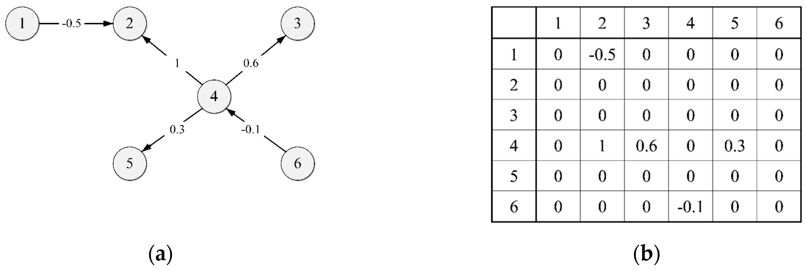
The direction of the edge represents the causal relationship between the nodes. An example of FCM is shown in Figure 2. The weight of the edge from node i to node j is denoted as w i j ( 1 , 1 ) . A positive w i j represents an excitatory relation from node i to node j, i.e., an increase (decrease) in C i will cause an increase (decrease) in C j , while a negative w i j represents an inhibitory relation. In addition, there is no relationship from node i to node j when the weight w i j is 0.
FCM with N variables (elements) can be expressed as a weighted matrix which is shown in Equation (16) [50,56]. According to the dataset used to construct the FCM, the value of the ith element, which is affected by the values of elements that have nonzero connections to the ith node, can be computed with Equation (17),
W = ( w 11 w 1 N w N 1 w N N ) , w i j [ cos 1 θ 1 , 1 ] ( 1 i N , 1 j N )
C i ( t + 1 ) = f ( i N w i j C j ( t ) )
where C i ( t + 1 ) and C j ( t ) are the value of the ith element at the (t + 1)th period, and the value of the jth element at the tth period, respectively. f ( ) represents the activation function that restricts the values of the node within the range of (0, 1). There are three widely used activation functions: The signum function, the trivalent function and the sigmoid function [57]. The sigmoid function has been used by most of the studies on FCM [58]. The sigmoid activation function is defined as follows:
f ( x ) = 1 1 + e λ 0 x
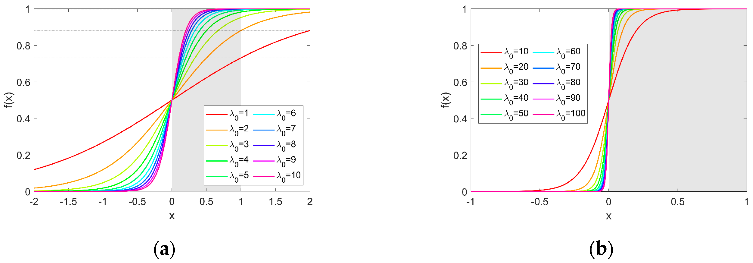
where λ 0 is the parameter that determines the steepness of the sigmoid function at values around 0. Figure 3 shows the function graph of f ( x ) with different λ 0 . Different λ 0 make the activation function work better for the weight matrix of the actual applications. However, it is the commonly used that λ 0 is set to 5.0 for the simulated study based on data generated using FCM in the some literature [59,60].

4.2. Fuzzy Cognitive Map with Offset

The activation function f ( x ) can restrict the node values within the range of (0, 1). But the effect of f ( x ) is greatly affected by the parameter λ 0 , and f ( x ) converts i N w i j C j ( t ) nonlinearly into (0, 1), which may cause data distortion. FCM with an offset is proposed to try to overcome the above problems. In FCM-O, the activation function is not used, and the offset is introduced to better learn the structure of a directed weighted graph to illustrate the concrete relationships between any pair of elements. The weighted matrix of FCM-O is the same as that of FCM as Equation (16). The dynamics of the node values in the FCM-O is simulated by using the following equation:
C i ( t + 1 ) = i N w i j C j ( t )   + O f f s e t i
where O f f s e t i is the offset of the ith element. The application of offset is to overcome the causal inference error caused by non-linear mapping of activation function could improve the fitting accuracy of the FCM, and the result of causal inference will be more intuitive without using the activation function. The processes of learning the structure of FCM and FCM-O is the same, which will be described in detail in the following Section 4.3.

4.3. Algorithm for Learning the Structure of FCM: Differential Evolution Algorithm

Most of the studies apply data-driven FCM learning algorithms focused on minimizing the simulation error [61,62,63] between an output sequence and historical data. A large number of meta-heuristic FCM learning algorithms exist [63], and can be found in the literature about differential evolution (DE) algorithm [64].
DE is a simple yet practical method for optimization problems proposed by Price and Storn [65]. Due to its simplicity, easy implementation, fast convergence and robustness, the DE algorithm has attracted more and more attention, and has been widely applied successfully, such as flow shop scheduling, piezoelectric performance optimization, economic optimization design, etc. [7,66,67]. A virtual population is used to form an initial solution in feasible space, and then recursive implementations of differential mutation, crossover, and greedy selection are executed until the termination condition is met. The solutions in the population evolve into a solution suitable for the dataset in this evolutionary process.
Finally, an optimal solution that can reasonably and accurately represent the FCM is formed. The solutions in the population generally represent the weight matrix and some parameters in FCM. In the greedy selection procedure, the min data error (fitness function) is used to evaluate the solutions in the population. The objective function in this research is shown as Equation (20).
min ( Data   Error ) = min ( 1 T N t = 1 T n = 1 N ( C n ( t ) C ˜ n ( t ) ) 2 )
where T is the period number of datasets. C n ( t ) and C ˜ n ( t ) are the value of the nth element at the tth moment in the dataset and the corresponding value returned from FCM, respectively. The smaller the data error is, the better.
LSHADE [68] contains the external archive and the mutation strategy ‘DE/current-to-pbest/1’ like JADE [69] and historical memory of successful control parameter settings like SHADE [70], and the strategy of linear population size reduction is applied. It secures the first rank (see http://www.ntu.edu.sg/home/EPNSugan/index_files/CEC2014/-CEC2014.htm) on real-parameter single objective numerical optimization in CEC2014 competition [71]. Due to the excellent performance of LSHADE in numeric optimization problems, it is selected to learn the structure of FCM. The parameter setting and specific implementation of LSHADE are referred to Ref [68].
Mutation is a change or perturbation with a random element on the population to locate better solutions. DE creates a mutant vector v i , G by utilizing one or more difference vectors. The mutation strategy in original DE is “rand/1”, which is expressed in Equation (21).
v i , G = x r 1 , G + F × ( x r 2 , G x r 3 , G )
Other common DE mutation strategies are as follows:
● “rand/2”:
v i , G = x r 1 , G + F × ( x r 2 , G x r 3 , G ) + F × ( x r 4 , G x r 5 , G )
● “best/1”:
v i , G = x b e s t , G + F × ( x r 1 , G x r 2 , G ) .
● “best/2”:
v i , G = x b e s t , G + F × ( x r 1 , G x r 2 , G ) + F × ( x r 3 , G x r 4 , G )
● “current to best/1”:
v i , G = x i , G + F × ( x b e s t , G x i , G ) + F × ( x r 1 , G x r 2 , G )
where the indices r 1 r 5 represent the random and mutually different integers generated within the range { 1 ,   N P } and different from the index i . x b e s t , G is the best individual in a current generation. Each strategy has a different ability to maintain the diversity of the population, which may increase/reduce the rate of convergence in the process of evolution.
LSHADE employs the mutation strategy ‘DE/current-to-pbest/1’ proposed in JADE, which is shown in Equation (26). ‘DE/current-to-pbest/1’ utilizes an optional external archive to diversify mutant vectors, and this achieves good performance over many benchmark functions. x p b e s t , G in Equation (26) denotes certain randomly-chosen vectors from the top 100 × p % individuals. DE/current-to-pbest/1 depends on the control parameter p in order to balance exploitation and exploration (small p behaves more greedily), and p is a constant set to 0.05 in JADE. JADE defines a set of archived inferior solutions A, and current population solutions P. x r 2 , G in mutation strategy is selected from the union PA. The archive A is initialized empty, and then inferior solutions (individuals) are added to the archive in each generation. The upper bound of archive size is fixed, and if the size exceeds the fixed threshold, these redundant solutions are randomly selected and removed from the external archive A to keep the upper bound of archive size equaling to the fixed threshold.
v i , G = x i , G + F × ( x p b e s t , G x i , G ) + F × ( x r 1 , G x r 2 , G )
After mutation, LSHADE generates a trial vector u i , G by a crossover operation to enhance the potential diversity of the population. In the basic version, the binomial crossover is a commonly used crossover operator operation in DE. It crosses the parent individual x i , G and the mutant vector v i , G to generate the trial vector u i , G . For each dimension j, it is implemented as follows:
u i , j , G = { v i , j , G if   rand [ 0 , 1 ]     C R i   or   j = j r a n d x i , j , G otherwise
where j r a n d   is an index of uniformly randomly chosen from [ 1 , D ] , which ensures that the trial vector u i , G gets at least one component from the mutant vector v i , G .
Selection compares the parent individual x i , G with the trial vector u i , G in terms of the objective function value to determine which vector may survive to the next generation. The operation in Equation (28) is called a successful update if the trial vector survives to the next generation.
x i , G + 1 = { x i , G otherwise u i , G if   u i , G   i s   b e t t e r   t h a n   x i , G
The corresponding solution and control parameters are called successful solution and successful control parameters, respectively. Otherwise, they are called unsuccessful update.
For the linear population size reduction, formula (29) shows the dynamic change of population size in LSHADE. N P m i n is set to the smallest possible value, such that the evolutionary operators can be applied in the case of L-SHADE, N P m i n = 4 because the DE/current-to-pbest/1 requires 4 individuals in Equation (26). N F E is the current number of fitness evaluations, and M A X N F E is the maximum number of fitness evaluations. Whenever N P G + 1 < N P G , the ( N P G N P G + 1 ) worst-ranking individuals are deleted from the population, and the external archive size | A | changes adaptively according to the dynamic population size, | A G | = round ( N P × r a r c ) , r a r c is the archive factor. Whenever the size of the archive exceeds the predefined archive size | A | , the randomly-selected elements are deleted to make space for the newly-inserted elements.
N P G + 1   =   round [ ( ( N P m i n N P i n i t M A X N F E ) N F E + N P i n i t ]
Control parameters in LSHADE are also updated in an adaptive manner as SHADE. F obeys a Cauchy distribution in which the location parameter is denoted by μF and the scale parameter equals to 0.1, FC (MF, 0.1). Cr obeys a normal distribution in which the mean value is denoted by MCr and standard deviation equals to 0.1, CrN (MCr, 0.1). If the values generated for F and Cr are outside the range (0, 1), Cr will be truncated to (0, 1), and F will be truncated to be 1 if F ≥ 1, or regenerated if F ≤ 0. The updating schemes of control parameters F and Cr are listed in Equations (30) and (31), respectively.
F i , G = randc ( M F i , G , 0.1 )
  C r i , G = { 0 if   M C r h , G = randn ( M C r h , G , 0.1 ) otherwise  
Success values of F and Cr in each generation are recorded and used to update S F and S C r . The updating schemes of control parameters M F and M C r are listed in Equations (32) and (33), respectively. As MCr is updated, if M C r h , G = “⊥” (where “⊥” denotes a special, “terminal value”) or max(SCr) = 0 (i.e., all elements of SCr are 0), M C r h , G + 1 is set to “⊥”. Thus, if MCr is assigned the terminal value “⊥”, then MCr will remain fixed at “⊥” until the end of the search.
This has the effect of locking Cr to 0 until the end of the search, causing the algorithm to enforce a “change-one-parameter-at-a-time” policy [72], which tends to slow down convergence, and is effective on multimodal problems.
M F h , G + 1   =   { mean W L ( S F ) if   S F M F h , G otherwise
M C r h , G + 1   =   { if   M C r h , G =   or   max ( S C r ) = 0 mean W A ( S C r ) if   S C r M C r h , G otherwise
where index h (1 < h < H) determines the position in the memory to update. The index h is initialized to 1 at the beginning. h is incremented whenever the entry ( M F h , M C R h ) is updated once. If h > H, h is set to 1. In the update Equations (32) and (33), the weighted mean m e a n W A ( S C r ) is computed according to Equation (35) referred to by Peng et al. [73]. The weighted Lehmer mean m e a n W L ( S F ) is computed using the formula below, and as with m e a n W A ( S C r ) :
mean W L ( S F ) = k | S F | w k   S F k 2 k | S F | w k   S F k
m e a n W A ( S C r ) = k = 1 | S C r | w k S C r k
{ w k = f k k = 1 | S C r | f k f k = | f ( u i , G ) f ( x i , G ) |

5. Case Study

5.1. Description of Research Area

The Yangtze River is the third longest river in the world, the largest river in China. The Three Gorges Reservoir (TGR) is the key backbone of the Yangtze River Basin (See as Figure 4), and the operation and management of TGR will inevitably affect the river basin ecosystem of the upper and lower reaches. The main parameters of TGR are listed in Table 1. In order to defend the coming flood in the flood season, the TGR empties storage capacity, and its water level dropped to 145 m at June 10. Then TGR begins to store water in September 1.

5.2. Dataset Acquisition and Preprocessing

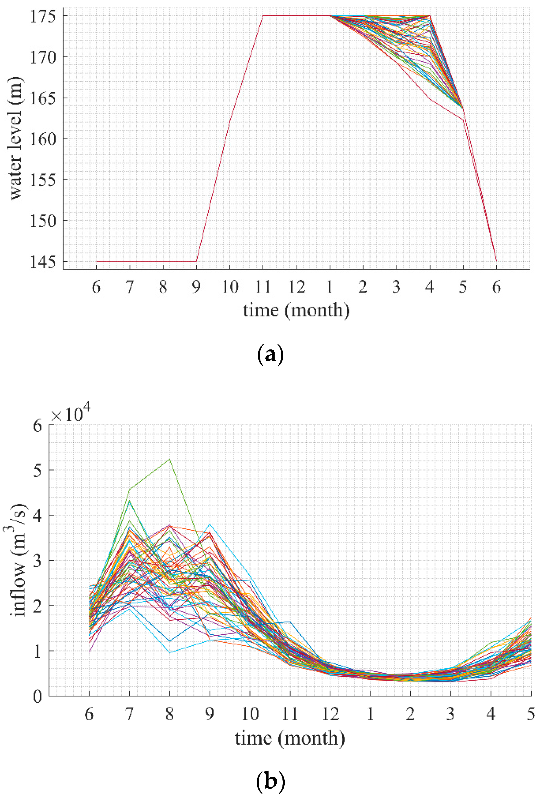
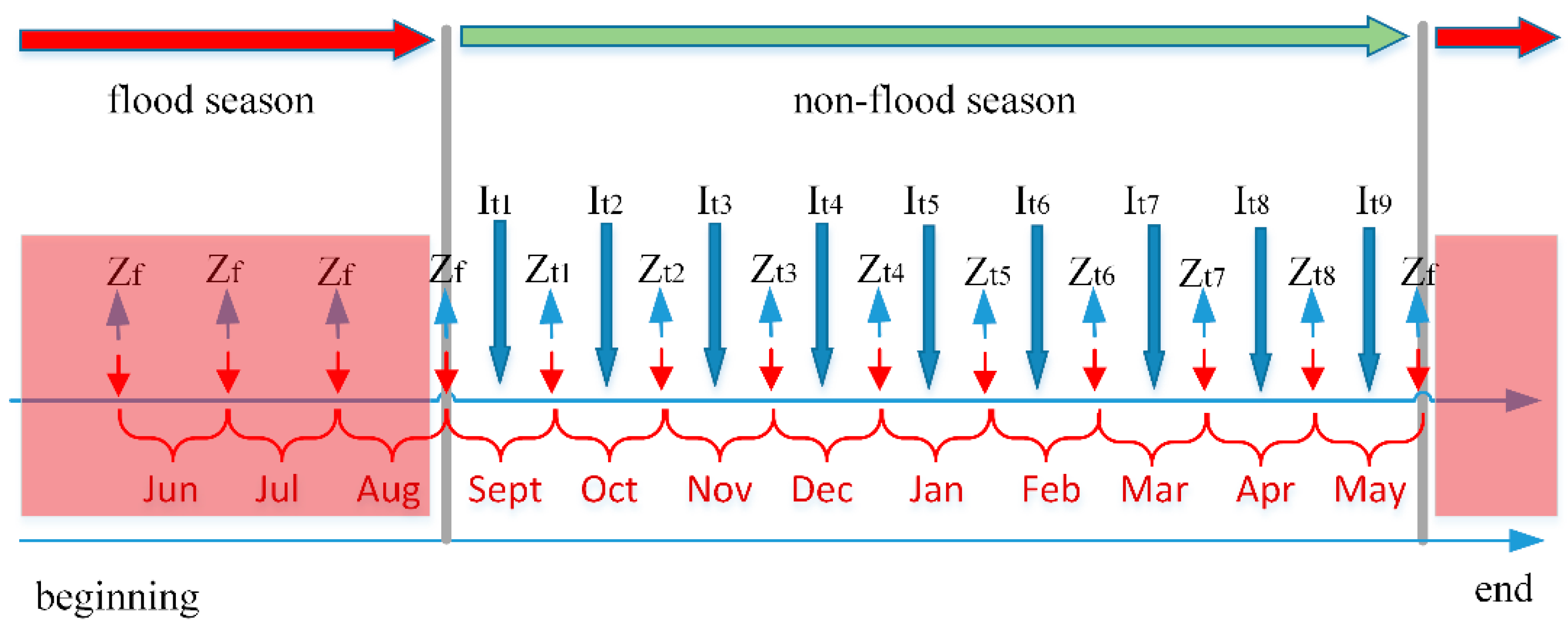
The main purpose of the study is to infer the causal relationship between the optimal control water level process { Z t * } and the inflow sequence { I t } in ROO. Section 3 describes in detail how to obtain an optimal control water level of reservoir operation by DP. The time step was monthly. Therefore, the scheduling period begins at June 1 and ends at June 1 of the next year. The initial water level Z i begin and terminal water level Z i end are set to 145 m. There is the historical inflow data of TGR for 55 years from 1959 to 2014. The objective of reservoir optimal operation is to maximize power generation as Equation (1). Figure 5 shows the inflow sequence { I t } and the optimal control water level process { Z t * } obtained by DP. From June to September, the water level of TGR is limited to the flood limit level (145 m) to prevent floods. Therefore, our research period focuses on the non-flood season, that is, September to May of the next year. { Z t * } and { I t } are illustrated in Figure 6 under the condition of a certain inflow sequence. Z f represents the flood limit level.
According to the regular “Optimal Operation Scheme of the Three Gorges” drawn up by Chengdu Engineering Corporation Limited, the water level control generally follows these regulations:
(1)
For power generation, the water level of TGR should be higher than 145 m, which is the dead water level. In addition, TGR should keep lower than the normal water level 175 m.
(2)
From July to early September, the TGR runs according to the flood control mode.
(3)
TGR begins to store water in September, and reaches 175 m by late October. TGR had better fill up quickly to improve the efficiency of power generation.
After the inflow sequence { I t } and the optimal control water level process { Z t * } for 55 years from 1959 to 2014 obtained by DP, all the data of { Z t * } and { I t } were preprocessed with Equations (37) and (38) to normalize the influence of each element and avoid the dominant elements whose absolute values are much larger than those of the other attributes. Z t , y and Z t , y * ( t = t 1 , , t T 1 ; y = 1 , Y ) are the normalized and pre-normalized optimal control water level of tth period with the yth inflow sequence. Z min and Z max are the minimum and maximum values of the optimal control water level under all the different inflow sequence conditions, respectively. T is the number of research periods. Y is the number of inflow sequence. I t , y and I t , y ( t = t 1 , , t T ; y = 1 , Y ) are the normalized and pre-normalized inflow of tth period with the yth inflow sequence. I min and I max are the minimum and maximum values of the optimal control water level under all the different inflow sequence conditions, respectively. The month corresponding to t = t 1 , , t T 1 is shown in Table 2. All the data were randomly divided into two parts (3/4 and 1/4) for training and testing. The final result is the FCM or FCM-O model with minimum data error.
{ Z t , y = ( Z t , y * Z min ) / ( Z max Z min ) Z min = min t [ t 1 , , t T 1 ] , y [ 1 , Y ] { Z t , y * } Z max = max t [ t 1 , , t T 1 ] , y [ 1 , Y ] { Z t , y * }
{ I t , y = ( I t , y I min ) / ( I max I min ) I min = min t [ t 1 , , t T ] , y [ 1 , Y ] { I t , y } I max = max t [ t 1 , , t T ] , y [ 1 , Y ] { I t , y }

5.3. Case Study and Discussion

In this case, FCM and FCM-O are established to infer the causal relationship between optimal control water level { Z t , y * } and inflow { I t , y } of ROO for TGR. In order to simplify the model, the relationship between inflows in each month is neglected. In addition, the recursive formula of DP in Section 3 shows that { Z t , y * } mainly depends on { I t , y } under given boundary conditions and constraints. Therefore, the model description of the above FCM and FCM-O can be simplified to the following expressions.
Z ˜ t Z , y = f ( t I = t 1 t T w t Z t I I t I , y )
Z ˜ t Z , y = t I = t 1 t T w t Z t I I t I , y   + O f f s e t t Z
where Z ˜ t Z , y is the tZth optimal control water level at the yth inflow sequence returned from FCM or FCM-O. w t Z t I represents the weight of the edge from the tIth inflow to the tZth optimal control water level. The corresponding objective function in this case is shown as Equation (25).
min ( Data   Error ) = min ( 1 ( T 1 ) Y t Z = t 1 t T y = 1 Y ( Z t Z , y Z ˜ t Z , y ) 2 )
LSHADE is selected to learn the structure of FCM, and the number of max fitness evaluations is set to 10,000 × D. D is the dimension of the problem. From Figure 6, it can be seen that the number of node Z t , y * is 8, and the number of node I t , y is 9 (T = 9). So D = 8 × 9 + 8 = 81 in FCM and FCM-O ( λ 0 of f ( x ) in FCM and O f f s e t t Z in FCM-O are needed to search for each Z t , y * ). Table 3 shows the min data error of FCM and FCM-O for training and testing. Compared with FCM in the min data error, FCM-O reduces 11.11% and 7.14% in the training and the testing, respectively. It shows that FCM-O is superior to FCM in terms of its minimum data error. The weight matrix and parameter of training results of FCM and FCM-O are shown in Table 4 and Table 5.
It can be seen from Figure 5a that Z 9 * , Z 10 * and Z 11 * maintain the same water level under different inflow sequences. TGR begins to store water in early September. According to the regulations, the water level at the end of September is not higher than 162 m, while Z 9 * reaches the upper boundaries of the constraint at 162 m. TGR is generally full to 175 m of normal water level from October to December, while Z 10 * and Z 11 * reaches the upper boundaries of the constraint at 175 m. It illustrates that TGR should impound water as fast as possible during the impoundment period, raising the head of power generation so as to increase the total power generation, which is consistent with the conclusions of many literatures [5,32,38,74]. Figure 5b shows that I 9 ranges in (12,000, 40,000) m3/s, while I 10 ranges in (11,000, 28,000) m3/s and I 11 ranges in (8,000, 16,000) m3/s. These indicate the value of Z 9 * , Z 10 * and Z 11 * are more affected by upper boundaries of the water level constraint constraints than by inflow. However, the weighting coefficients of I t , y to Z 9 * , Z 10 * , and Z 11 * in FCM are 1 or −1 in Table 4, which shows that Z 9 * , Z 10 * and Z 11 * are greatly affected by I t , y . The conclusions obtained by FCM do not match the accepted conclusions that Z 9 * , Z 10 * and Z 11 * are more affected by constraints than by inflow, and the weighting coefficients of I t , y to Z 9 * , Z 10 * and Z 11 * in FCM-O are 0, which seems reasonable. The reason for the above causal inference errors in FCM lies in the inability of the activation function f ( x ) to deal with variables with offsets that are not 1 or −1. All of those shows that FCM-O is more competent than FCM in the causal relationship between optimal control water level and inflow in ROO both in min data error and reasonableness of results.
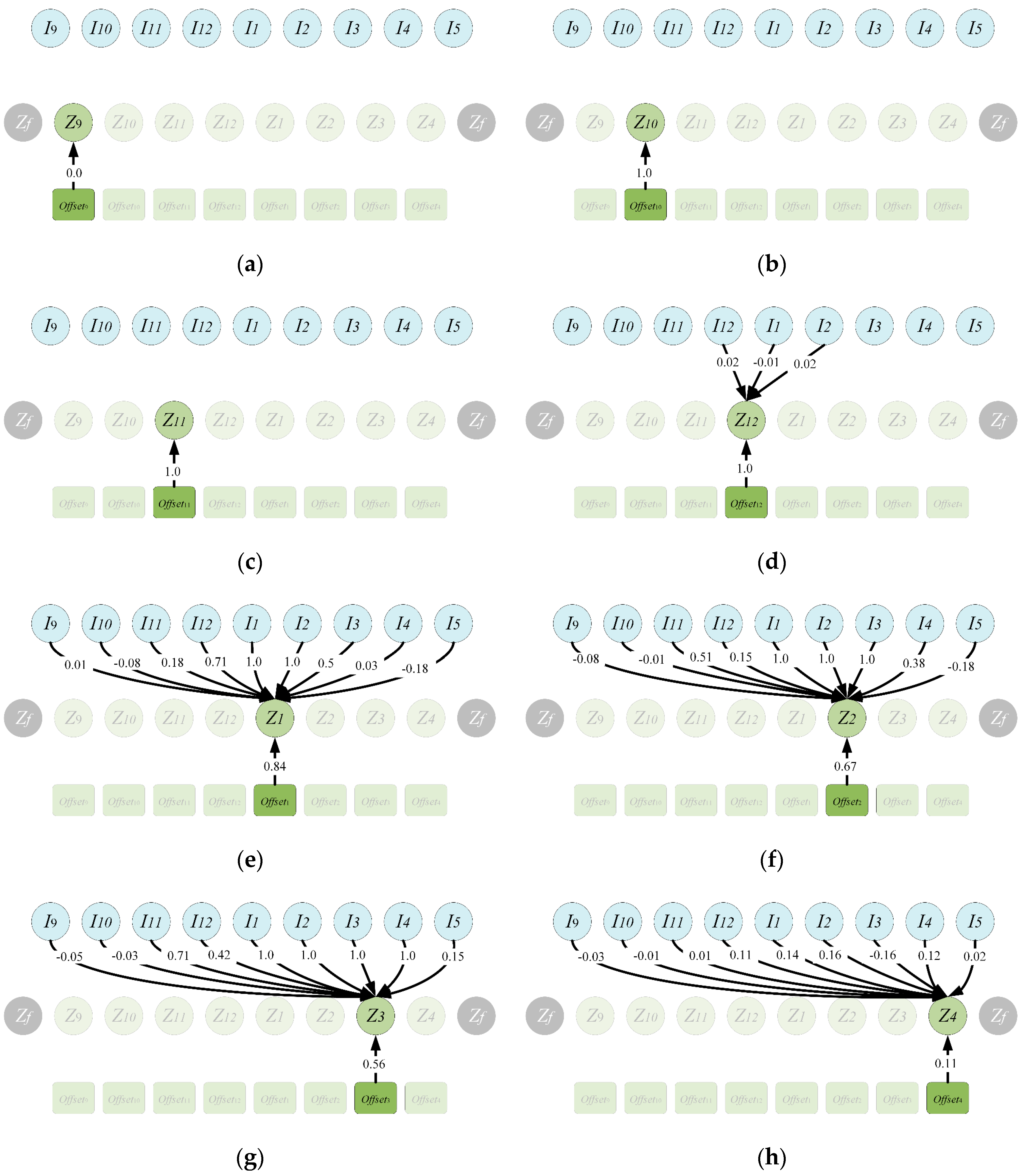
To analyze the results of FCM-O, the weight matrices corresponding to all subfigures are shown in Figure 6. Because the relationship between inflows is neglected, and the optimal control water level depends on the sequence of inflow, and are unrelated to the adjacent water level, the optimal control water level only pays attention to the in degree and offset, and all out degrees are 0.
Table 6 shows the in degree and offset of each Z t * of Figure 7. Z 9 * , Z 10 * , Z 11 * and Z 12 * need to reach higher operating water levels, which are more affected by constraints than by inflow. So there is no inflow but only offset acting on Z 9 * , Z 10 * , Z 11 * and Z 12 * , as shown in Figure 7a–d. Z 1 * , Z 2 * and Z 3 * reflect the optimal control water level in the early stage of the water supply period, and Z 1 * , Z 2 * and Z 3 * range in (145, 175) m. In the early stage of the water supply period, TRG should reduce the discharge as much as possible and maintain a higher head, so as to increase power generation under the premise of meeting the minimum discharge constraint. Therefore, Z 1 * , Z 2 * and Z 3 * are mainly affected by the inflow in recent months. The larger the inflow, the smaller the amount of water that the reservoir needs to release, and correspondingly, Z 1 * , Z 2 * and Z 3 * will be higher. The inflow in recent months has shown positive effects to Z 1 * , Z 2 * and Z 3 * . Z 4 * reflects the optimal control water level at the end of the water supply period (before the flood season). There are many elements to be considered in Z 4 * . First, Z 4 * needs to maintain a high water level to ensure a higher head, thereby increasing power generation. Secondly, Z 4 * needs to avoid too high a water level to produce discarded water when emptying the reservoir before flood season. Therefore, Z 4 * has a narrow range and is less affected by inflow in different months as shown in Figure 5a and Figure 6h.
The results in this research are consistent with some abovementioned literatures. Moreover, our studies made these conclusions quantitative. Meanwhile, we found some details that were overlooked previously, such as the conclusion that Z 9 * , Z 10 * and Z 11 * are more affected by constraints than by inflow, and the inflow in recent months has shown positive effect to Z 1 * , Z 2 * and Z 3 * . In addition, we can use this relationship to estimate the optimal control water level with inflow in FCM-O.

6. Conclusions

A new FCM with offset was proposed to try to infer the causal relationship between the optimal control water level and the inflow of ROO. To test its performance, the FCM and FCM-O of ROO for TGR are established. The optimal control water levels of TGR were obtained by DP with the historical inflow data for 55 years from 1959 to 2014. Then all the data of this optimal control water level and inflow were randomly divided into two parts (3/4 and 1/4) for training and testing. The FCM or FCM-O model were trained with minimum data error by LSHADE. The experimental results show that, compared with FCM in the min data error, FCM-O reduces 11.11% and 7.14% in the training and the testing, respectively. In addition, FCM-O can deduce that the optimal control water level from September to December needs to be raised as much as possible, which are mainly restricted by constraints and are not affected by inflow. The optimal control water level from January to March also needs to maintain a high water level, and the inflow in recent months has a positive effect upon it. The optimal controlled water level at the end of April is at the end of the water supply period and near the flood season. The optimal control water level at the end of April needs to maintain an appropriate high water level, so as to avoid the risk of discarding water while guaranteeing high water head to increase power generation. In addition, the relationship obtained by FCM-O can be used to estimate the optimal control water level with inflow.

Author Contributions

Y.L. completed the revision of the article and language editing. Z.H. designed and conducted the experiments. Y.L., Z.H. and J.Z. wrote the draft of the paper. Y.L., C.L. and H.Q. proposed the main structure of this study. B.J. prepared the figures for this paper. K.F., F.H., and G.L. provided useful advice and made some corrections. All authors read and approved the final manuscript.

Funding

This work was funded by the National Key R&D Program of China (2016YFC0402210), the Fundamental Research Funds for the Central Universities (2017KFYXJJ192).

Acknowledgments

Special thanks are given to the anonymous reviewers and editors for their constructive comments.

Conflicts of Interest

The authors declare no conflict of interest.

References

  1. Wang, H.; Yang, Z.; Saito, Y.; Liu, J.P.; Sun, X. Interannual and seasonal variation of the Huanghe (Yellow River) water discharge over the past 50 years: Connections to impacts from ENSO events and dams. Glob. Planet. Chang. 2006, 50, 212–225. [Google Scholar] [CrossRef]
  2. Feng, Z.; Niu, W.; Cheng, C. China’s large-scale hydropower system: Operation characteristics, modeling challenge and dimensionality reduction possibilities. Renew. Energy 2019, 136, 805–818. [Google Scholar] [CrossRef]
  3. Babel, M.S.; Dinh, C.N.; Mullick, M.R.A.; Nanduri, U.V. Operation of a hydropower system considering environmental flow requirements: A case study in La Nga river basin, Vietnam. J. Hydro-Environ. Res. 2012, 6, 63–73. [Google Scholar] [CrossRef]
  4. Feng, Z.K.; Niu, W.J.; Wang, W.C.; Zhou, J.Z.; Cheng, C.T. A mixed integer linear programming model for unit commitment of thermal plants with peak shaving operation aspect in regional power grid lack of flexible hydropower energy. Energy 2019, 175, 618–629. [Google Scholar] [CrossRef]
  5. Zhao, T.; Zhao, J.; Yang, D. Improved dynamic programming for hydropower reservoir operation. J. Water Resour. Plan. Manag. 2012, 140, 365–374. [Google Scholar] [CrossRef]
  6. Zhao, T.; Cai, X.; Lei, X.; Wang, H. Improved dynamic programming for reservoir operation optimization with a concave objective function. J. Water Resour. Plan. Manag. 2011, 138, 590–596. [Google Scholar] [CrossRef]
  7. He, Z.; Zhou, J.; Qin, H.; Jia, B.; Lu, C. Long-term joint scheduling of hydropower station group in the upper reaches of the Yangtze River using partition parameter adaptation differential evolution. Eng. Appl. Artif. Intell. 2019, 81, 1–13. [Google Scholar] [CrossRef]
  8. Liu, Y.; Qin, H.; Mo, L.; Wang, Y.; Chen, D.; Pang, S.; Yin, X. Hierarchical Flood Operation Rules Optimization Using Multi-Objective Cultured Evolutionary Algorithm Based on Decomposition. Water Resour. Manag. 2019, 33, 337–354. [Google Scholar] [CrossRef]
  9. Wang, Q.; Zhou, J.; Huang, K.; Dai, L.; Zha, G.; Chen, L.; Qin, H. Risk assessment and decision-making based on mean-CVaR-entropy for flood control operation of large scale reservoirs. Water 2019, 11, 649. [Google Scholar] [CrossRef]
  10. Huang, K.; Ye, L.; Chen, L.; Wang, Q.; Dai, L.; Zhou, J.; Singh, V.P.; Huang, M.; Zhang, J. Risk analysis of flood control reservoir operation considering multiple uncertainties. J. Hydrol. 2018, 565, 672–684. [Google Scholar] [CrossRef]
  11. Liu, P.; Li, L.; Guo, S.; Xiong, L.; Zhang, W.; Zhang, J.; Xu, C.Y. Optimal design of seasonal flood limited water levels and its application for the Three Gorges Reservoir. J. Hydrol. 2015, 527, 1045–1053. [Google Scholar] [CrossRef]
  12. Chen, D.; Chen, Q.; Leon, A.S.; Li, R. A Genetic Algorithm Parallel Strategy for Optimizing the Operation of Reservoir with Multiple Eco-environmental Objectives. Water Resour. Manag. 2016, 30, 2127–2142. [Google Scholar] [CrossRef]
  13. Giuliani, M.; Castelletti, A.; Pianosi, F.; Mason, E.; Reed, P.M. Curses, tradeoffs, and scalable management: Advancing evolutionary multiobjective direct policy search to improve water reservoir operations. J. Water Resour. Plan. Manag. 2015, 142, 4015050. [Google Scholar] [CrossRef]
  14. Feng, Z.; Niu, W.; Cheng, C. Optimization of hydropower reservoirs operation balancing generation benefit and ecological requirement with parallel multi-objective genetic algorithm. Energy 2018, 153, 706–718. [Google Scholar] [CrossRef]
  15. He, Z.; Zhou, J.; Mo, L.; Qin, H.; Xiao, X.; Jia, B.; Wang, C. Multiobjective reservoir operation optimization using improved multiobjective dynamic programming based on reference lines. IEEE Access 2019, 7, 103473–103484. [Google Scholar] [CrossRef]
  16. Bai, T.; Wei, J.; Chang, F.J.; Yang, W.; Huang, Q. Optimize multi-objective transformation rules of water-sediment regulation for cascade reservoirs in the Upper Yellow River of China. J. Hydrol. 2019, 577, 123987. [Google Scholar] [CrossRef]
  17. Tsai, W.P.; Chang, F.J.; Chang, L.C.; Herricks, E.E. AI techniques for optimizing multi-objective reservoir operation upon human and riverine ecosystem demands. J. Hydrol. 2015, 530, 634–644. [Google Scholar] [CrossRef]
  18. Chang, L.C.; Chang, F.J. Multi-objective evolutionary algorithm for operating parallel reservoir system. J. Hydrol. 2009, 377, 12–20. [Google Scholar] [CrossRef]
  19. Jiang, Z.; Qin, H.; Ji, C.; Hu, D.; Zhou, J. Effect Analysis of Operation Stage Difference on Energy Storage Operation Chart of Cascade Reservoirs. Water Resour. Manag. 2019, 33, 1349–1365. [Google Scholar] [CrossRef]
  20. Jiang, Z.; Qiao, Y.; Chen, Y.; Ji, C. A New Reservoir Operation Chart Drawing Method Based on Dynamic Programming. Energies 2018, 11, 3355. [Google Scholar] [CrossRef]
  21. Feng, Z.K.; Niu, W.J.; Zhang, R.; Wang, S.; Cheng, C.T. Operation rule derivation of hydropower reservoir by k-means clustering method and extreme learning machine based on particle swarm optimization. J. Hydrol. 2019, 576, 229–238. [Google Scholar] [CrossRef]
  22. Niu, W.J.; Feng, Z.K.; Feng, B.F.; Min, Y.W.; Cheng, C.T.; Zhou, J.Z. Comparison of multiple linear regression, artificial neural network, extreme learning machine, and support vector machine in deriving operation rule of hydropower reservoir. Water 2019, 11, 88. [Google Scholar] [CrossRef]
  23. Feng, M.; Liu, P.; Guo, S.; Gui, Z.; Zhang, X.; Zhang, W.; Xiong, L. Identifying changing patterns of reservoir operating rules under various inflow alteration scenarios. Adv. Water Resour. 2017, 104, 23–36. [Google Scholar] [CrossRef]
  24. Fu, W.; Wang, K.; Zhang, C.; Tan, J. A hybrid approach for measuring the vibrational trend of hydroelectric unit with enhanced multi-scale chaotic series analysis and optimized least squares support vector machine. Trans. Inst. Meas. Control 2019, 41, 4436–4449. [Google Scholar] [CrossRef]
  25. He, Z.; Zhou, J.; Sun, N.; Jia, B.; Qin, H. Integrated scheduling of hydro, thermal and wind power with spinning reserve. Energy Procedia 2019, 158, 6302–6308. [Google Scholar] [CrossRef]
  26. Chang, L.; Chang, F. Intelligent control for modelling of real-time reservoir operation. Hydrol. Process. 2001, 15, 1621–1634. [Google Scholar] [CrossRef]
  27. Jiang, Z.; Li, A.; Ji, C.; Qin, H.; Yu, S.; Li, Y. Research and application of key technologies in drawing energy storage operation chart by discriminant coefficient method. Energy 2016, 114, 774–786. [Google Scholar] [CrossRef]
  28. Yoo, J.H. Maximization of hydropower generation through the application of a linear programming model. J. Hydrol. 2009, 376, 182–187. [Google Scholar] [CrossRef]
  29. Catalão, J.P.; Pousinho, H.M.I.; Mendes, V.M.F. Scheduling of head-dependent cascaded hydro systems: Mixed-integer quadratic programming approach. Energy Convers. Manag. 2010, 51, 524–530. [Google Scholar] [CrossRef]
  30. Jiang, Z.; Qin, H.; Ji, C.; Feng, Z.; Zhou, J. Two dimension reduction methods for multi-dimensional dynamic programming and its application in cascade reservoirs operation optimization. Water 2017, 9, 634. [Google Scholar] [CrossRef]
  31. Nanda, J.; Bijwe, P.R. Optimal Hydrothermal Scheduling with Cascaded Plants Using Progressive Optimality Algorithm. IEEE Trans. Power Appar. Syst. 1981, PAS-100, 2093–2099. [Google Scholar] [CrossRef]
  32. Wang, C.; Zhou, J.; Lu, P.; Yuan, L. Long-term scheduling of large cascade hydropower stations in Jinsha River, China. Energy Convers. Manag. 2015, 90, 476–487. [Google Scholar] [CrossRef]
  33. Lee, J.; Labadie, J.W. Stochastic optimization of multireservoir systems via reinforcement learning. Water Resour. Res. 2007, 43, W11408. [Google Scholar] [CrossRef]
  34. Cheng, C.T.; Liao, S.L.; Tang, Z.T.; Zhao, M.Y. Comparison of particle swarm optimization and dynamic programming for large scale hydro unit load dispatch. Energy Convers. Manag. 2009, 50, 3007–3014. [Google Scholar] [CrossRef]
  35. Yuan, X.; Yuan, Y. Application of cultural algorithm to generation scheduling of hydrothermal systems. Energy Convers. Manag. 2006, 47, 2192–2201. [Google Scholar] [CrossRef]
  36. Arvanitidits, N.V.; Rosing, J. Composite representation of a multireservoir hydroelectric power system. IEEE Trans. Power Appar. Syst. 1970, PAS-89, 319–326. [Google Scholar] [CrossRef]
  37. Brandao, J.L.B. Performance of the equivalent reservoir modelling technique for multi-reservoir hydropower systems. Water Resour. Manag. 2010, 24, 3101–3114. [Google Scholar] [CrossRef]
  38. Zhao, T.; Zhao, J.; Liu, P.; Lei, X. Evaluating the marginal utility principle for long-term hydropower scheduling. Energy Convers. Manag. 2015, 106, 213–223. [Google Scholar] [CrossRef] [Green Version]
  39. Zhao, T.; Zhao, J.; Lei, X.; Wang, X.; Wu, B. Improved Dynamic Programming for Reservoir Flood Control Operation. Water Resour. Manag. 2017, 31, 2047–2063. [Google Scholar] [CrossRef]
  40. Kosko, B. Fuzzy cognitive maps. Int. J. Man Mach. Stud. 1986, 24, 65–75. [Google Scholar] [CrossRef]
  41. Papakostas, G.A.; Koulouriotis, D.E.; Polydoros, A.S.; Tourassis, V.D. Towards Hebbian learning of Fuzzy Cognitive Maps in pattern classification problems. Expert Syst. Appl. 2012, 39, 10620–10629. [Google Scholar] [CrossRef]
  42. Papageorgiou, E.; Stylios, C.; Groumpos, P. Fuzzy cognitive map learning based on nonlinear Hebbian rule. In Proceedings of the Australasian Joint Conference on Artificial Intelligence, Perth, WA, Australia, 3–5 December 2003; pp. 256–268. [Google Scholar]
  43. Salmeron, J.L.; Mansouri, T.; Moghadam, M.R.S.; Mardani, A. Learning Fuzzy Cognitive Maps with modified asexual reproduction optimisation algorithm. Knowl. Based Syst. 2019, 163, 723–735. [Google Scholar] [CrossRef]
  44. Poczeta, K.; Kubuś, Ł.; Yastrebov, A. Analysis of an evolutionary algorithm for complex fuzzy cognitive map learning based on graph theory metrics and output concepts. Biosystems 2019, 179, 39–47. [Google Scholar] [CrossRef] [PubMed]
  45. Chen, Y.; Mazlack, L.J.; Minai, A.A.; Lu, L.J. Inferring causal networks using fuzzy cognitive maps and evolutionary algorithms with application to gene regulatory network reconstruction. Appl. Soft Comput. 2015, 37, 667–679. [Google Scholar] [CrossRef]
  46. Mendonça, M.; Angelico, B.; Arruda, L.V.R.; Neves, F., Jr. A dynamic fuzzy cognitive map applied to chemical process supervision. Eng. Appl. Artif. Intell. 2013, 26, 1199–1210. [Google Scholar] [CrossRef]
  47. Stylios, C.D.; Groumpos, P.P. Modeling complex systems using fuzzy cognitive maps. IEEE Trans. Syst. Man Cybern. Part A Syst. Hum. 2004, 34, 155–162. [Google Scholar] [CrossRef]
  48. Hossain, S.; Brooks, L. Fuzzy cognitive map modelling educational software adoption. Comput. Educ. 2008, 51, 1569–1588. [Google Scholar] [CrossRef]
  49. Kok, K. The potential of Fuzzy Cognitive Maps for semi-quantitative scenario development, with an example from Brazil. Glob. Environ. Chang. 2009, 19, 122–133. [Google Scholar] [CrossRef]
  50. Zhang, K.; Pan, Q.; Yu, D.; Wang, L.; Liu, Z.; Li, X.; Liu, X. Systemically modeling the relationship between climate change and wheat aphid abundance. Sci. Total Environ. 2019, 674, 392–400. [Google Scholar] [CrossRef]
  51. Wen, X.; Zhou, J.; He, Z.; Wang, C. Long-term scheduling of large-scale cascade hydropower stations using improved differential evolution algorithm. Water 2018, 10, 383. [Google Scholar] [CrossRef]
  52. Bellman, R.E.; Dreyfus, S.E. Applied Dynamic Programming; Princeton University Press: Princeton, NJ, USA, 2015; Volume 2050, ISBN 1400874653. [Google Scholar]
  53. Yakowitz, S. Dynamic programming applications in water resources. Water Resour. Res. 1982, 18, 673–696. [Google Scholar] [CrossRef]
  54. Labadie, J.W. Optimal operation of multireservoir systems: State-of-the-art review. J. Water Resour. Plan. Manag. 2004, 130, 93–111. [Google Scholar] [CrossRef]
  55. Loucks, D.P.; Van Beek, E.; Stedinger, J.R.; Dijkman, J.P.M.; Villars, M.T. Water Resources Systems Planning and Management: An Introduction to Methods, Models and Applications; Unesco: Paris, France, 2005; ISBN 9231039989. [Google Scholar]
  56. Wu, K.; Liu, J. Robust learning of large-scale fuzzy cognitive maps via the lasso from noisy time series. Knowl. Based Syst. 2016, 113, 23–38. [Google Scholar] [CrossRef]
  57. Tsadiras, A.K. Comparing the inference capabilities of binary, trivalent and sigmoid fuzzy cognitive maps. Inf. Sci. 2008, 178, 3880–3894. [Google Scholar] [CrossRef]
  58. Bueno, S.; Salmeron, J.L. Benchmarking main activation functions in fuzzy cognitive maps. Expert Syst. Appl. 2009, 36, 5221–5229. [Google Scholar] [CrossRef]
  59. Stach, W.; Pedrycz, W.; Kurgan, L.A. Learning of fuzzy cognitive maps using density estimate. IEEE Trans. Syst. Man Cybern. Part B (Cybern.) 2012, 42, 900–912. [Google Scholar] [CrossRef] [PubMed]
  60. Chen, Y.; Mazlack, L.; Lu, L. Learning fuzzy cognitive maps from data by ant colony optimization. In Proceedings of the 14th Annual Conference on Genetic and Evolutionary Computation, Philadelphia, PA, USA, 7–11 July 2012; pp. 9–16. [Google Scholar]
  61. Papageorgiou, E.I. Learning algorithms for fuzzy cognitive maps—A review study. IEEE Trans. Syst. Man Cybern. Part C (Appl. Rev.) 2011, 42, 150–163. [Google Scholar] [CrossRef]
  62. Stach, W.; Kurgan, L.; Pedrycz, W. A divide and conquer method for learning large fuzzy cognitive maps. Fuzzy Sets Syst. 2010, 161, 2515–2532. [Google Scholar] [CrossRef]
  63. Stach, W.; Kurgan, L.; Pedrycz, W.; Reformat, M. Evolutionary development of fuzzy cognitive maps. In Proceedings of the The 14th IEEE International Conference on Fuzzy Systems, Reno, NV, USA, 25 May 2005; pp. 619–624. [Google Scholar]
  64. Das, S.; Suganthan, P.N. Differential evolution: A survey of the state-of-the-art. IEEE Trans. Evol. Comput. 2011, 15, 4–31. [Google Scholar] [CrossRef]
  65. Storn, R.; Price, K. Differential Evolution—A Simple and Efficient Heuristic for global Optimization over Continuous Spaces. J. Glob. Optim. 1997, 11, 341–359. [Google Scholar] [CrossRef]
  66. Li, J.Q.; Sang, H.Y.; Han, Y.Y.; Wang, C.G.; Gao, K.Z. Efficient multi-objective optimization algorithm for hybrid flow shop scheduling problems with setup energy consumptions. J. Clean. Prod. 2018, 181, 584–598. [Google Scholar] [CrossRef]
  67. Tey, K.S.; Mekhilef, S.; Seyedmahmoudian, M.; Horan, B.; Oo, A.T.; Stojcevski, A. Improved differential evolution-based MPPT algorithm using SEPIC for PV systems under partial shading conditions and load variation. IEEE Trans. Ind. Inform. 2018, 14, 4322–4333. [Google Scholar] [CrossRef]
  68. Tanabe, R.; Fukunaga, A.S. Improving the search performance of SHADE using linear population size reduction. In Proceedings of the Evolutionary Computation, Beijing, China, 6–11 July 2014; pp. 1658–1665. [Google Scholar]
  69. Zhang, J.; Sanderson, A.C. JADE: Adaptive Differential Evolution With Optional External Archive. IEEE Trans. Evol. Comput. 2009, 13, 945–958. [Google Scholar] [CrossRef]
  70. Tanabe, R.; Fukunaga, A. Success-history based parameter adaptation for Differential Evolution. In Proceedings of the Evolutionary Computation, Cancun, Mexico, 20–23 June 2013; pp. 71–78. [Google Scholar]
  71. Liang, J.J.; Qu, B.Y.; Suganthan, P.N. Problem Definitions and Evaluation Criteria for the CEC 2014 Special Session and Competition on Single Objective Real-Parameter Numerical Optimization; Technical Report 201311; Zhengzhou University and Nanyang Technological University: Singapore, 2013. [Google Scholar]
  72. Piotrowski, A.P.; Napiorkowski, J.J. Step-by-step improvement of JADE and SHADE-based algorithms: Success or failure? Swarm Evol. Comput. 2018, 43, 88–108. [Google Scholar] [CrossRef]
  73. Peng, F.; Tang, K.; Chen, G.; Yao, X. Multi-start JADE with knowledge transfer for numerical optimization. In Proceedings of the Eleventh Conference on Congress on Evolutionary Computation, Trondheim, Norway, 18–21 May 2009; pp. 1889–1895. [Google Scholar]
  74. Zhou, J.; Xie, M.; He, Z.; Qin, H.; Yuan, L. Medium-Term Hydro Generation Scheduling (MTHGS) with Chance Constrained Model (CCM) and Dynamic Control Model (DCM). Water Resour. Manag. 2017, 31, 3543–3555. [Google Scholar] [CrossRef]
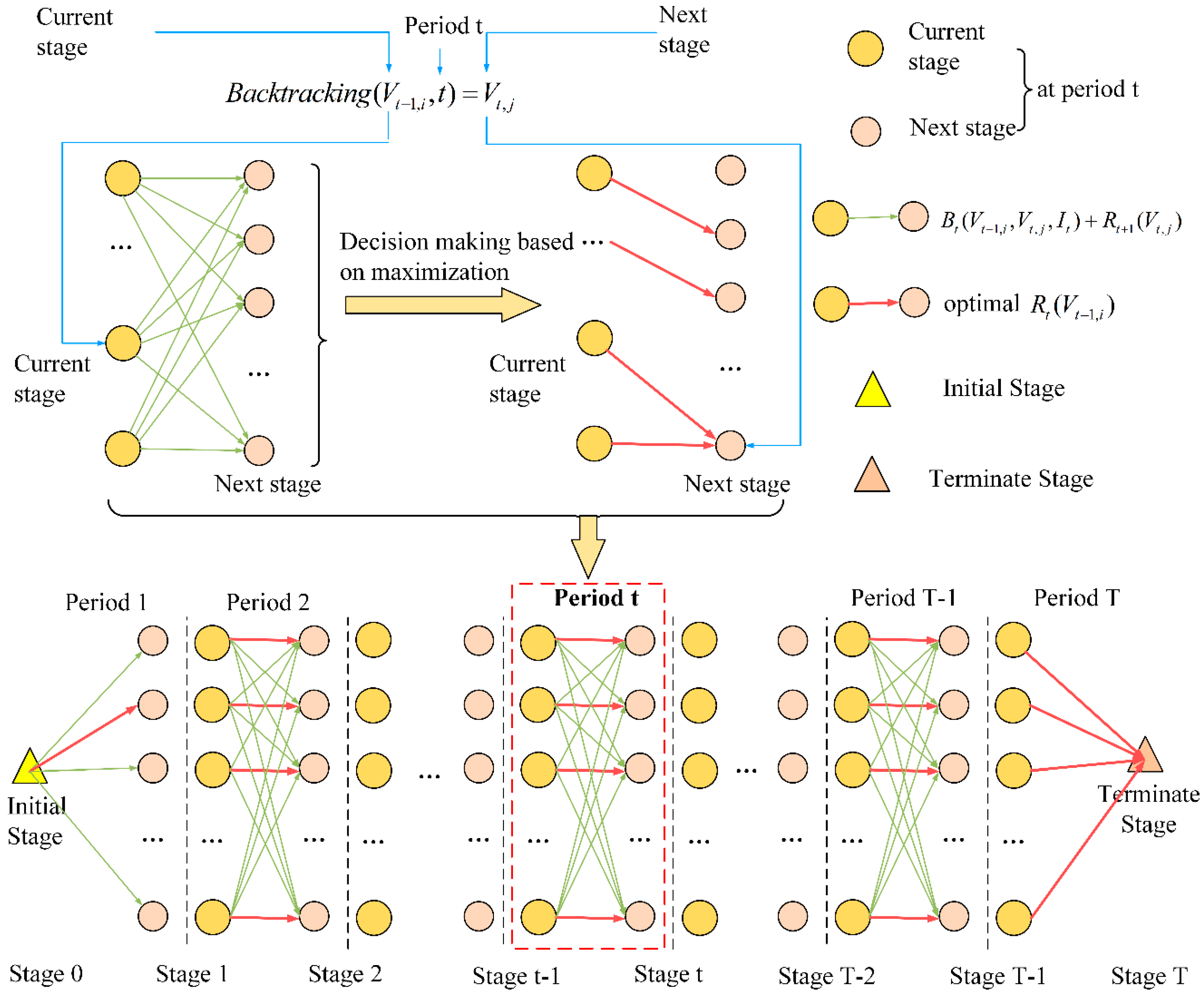
Figure 1. The decision-making process of dynamic programming (DP) for reservoir operation.
Water 11 02147 g001
Figure 2. An example of a fuzzy cognitive map (FCM) and its equivalent weight matrix. (a) Graph Representation, (b) Matrix Representation.
Water 11 02147 g002
Figure 3. The function diagram of f ( x ) with different λ 0 ; (a) λ 0 = 1, 2, 3, 4, 5, 6, 8, 10, (b) λ 0 = 10, 20, 30, 40, 50, 60, 80, 100.
Water 11 02147 g003
Figure 4. The location of the research area in China.
Water 11 02147 g004
Figure 5. The optimal control water level and inflow of the dataset from 1959 to 2014. (a) optimal control water level { Z t * }, (b) inflow sequence { I t }.
Water 11 02147 g005
Figure 6. The schematic diagram of { Z t * } and { I t } under the condition of a certain inflow.
Water 11 02147 g006
Figure 7. The relationship between { Z t * } and { I t } obtain by FCM-O. (a) Z 9 * , (b) Z 10 * , (c) Z 11 * , (d) Z 12 * , (e) Z 1 * , (f) Z 2 * , (g) Z 3 * , (h) Z 4 * .
Water 11 02147 g007
Table 1. Main parameters of the Three Gorges Reservoir (TGR).
ParameterTGR
Adjustment abilitySeason
Total reservoir capacity (billion m3)39.30
Regulating storage (billion m3)16.50
Hydro plant discharge range(m3/s)(98, 800, 4500)
Upriver water level range (m)(175, 145)
Installed capacity (MW)22,400
Normal water level (m)175
Maximum water level amplitude(m/d)0.6
Table 2. The month corresponding to t = t 1 , , t T 1 .
tt1 t 2 t 3 t 4 t 5 t 6 t 7 t 8 t 9
month910111212345
SeptOctNovDecJanFebMarAprMay
Table 3. The min data error of the fuzzy cognitive map (FCM) and fuzzy cognitive map with offset (FCM-O) for training and testing.
MethodTrainingTesting
min data errorFCM0.00450.0056
FCM-O0.00400.0052
FCM-O vs. FCM in the reduction of min data error11.11%7.14%
Table 4. The weight matrix and parameter of training results of FCM.
Z9Z10Z11Z12Z1Z2Z3Z4
I9−1.001.001.001.000.20−0.03−0.30−0.24
I10−1.001.001.001.00−0.09−0.13−0.07−0.16
I11−1.001.001.001.001.001.000.72−0.16
I12−1.001.001.001.001.000.620.79−0.40
I1−1.001.001.001.001.001.001.00−1.00
I2−1.001.001.001.001.001.001.000.36
I3−1.001.001.001.001.001.001.00−1.00
I4−1.001.001.001.001.001.001.000.09
I5−1.001.001.001.000.01−0.290.10−0.34
λ05.005.005.005.005.005.005.005.00
Table 5. The weight matrix and parameter of training results of FCM.
Z9Z10Z11Z12Z1Z2Z3Z4
I90.000.000.000.000.01−0.08−0.05−0.03
I100.000.000.000.00−0.08−0.01−0.03−0.01
I110.000.000.000.000.180.510.710.01
I120.000.000.000.020.710.150.420.11
I10.000.000.00−0.011.001.001.000.14
I20.000.000.000.021.001.001.000.16
I30.000.000.000.000.501.001.00−0.16
I40.000.000.000.000.030.381.000.12
I50.000.000.000.00−0.18−0.180.150.02
O f f s e t t Z 0.001.001.001.000.840.670.560.11
Table 6. The in degree and offset of each Z t * of FCM-O.
In DegreeIn Element O f f s e t t Z
Z90 0
Z100 1
Z110 1
Z123I12, I1, I21
Z19I9, I10, I11, I12,
I1, I2, I3, I4, I5
0.84
Z29I9, I10, I11, I12,
I1, I2, I3, I4, I5
0.67
Z39I9, I10, I11, I12,
I1, I2, I3, I4, I5
0.56
Z49I9, I10, I11, I12,
I1, I2, I3, I4, I5
0.11