Optimization Difficulty Indicator and Testing Framework for Water Distribution Network Complexity

Abstract

In the last three decades, benchmark water distribution networks (WDNs) have provided a common testbed for new optimization algorithms and design approaches. However, deriving generalized and reliable conclusions from such benchmark WDNs is difficult because their optimization difficulty levels (ODLs) are either too low or too high (i.e., biased). Final solutions do not consistently converge to a global optimum for a WDN problem with a high ODL. In addition, little effort has been given to quantifying and comparing the ODLs of WDNs with different characteristics and conditions. In this study, an ODL indicator was developed for WDNs: the coefficient of variation of the final solution fitness values. An ODL quantification framework was also developed with two phases: (1) generating network layouts with various topological characteristics, and (2) quantifying the statistics of the final solution quality and ODL by using a global parallel genetic algorithm. The proposed indicator and framework were applied to the design of a dense-grid B-city network and large C network, and the results demonstrated their applicability to generating a WDN benchmark problem with the target ODL.

1. Introduction

In the last three decades, many metaheuristic optimization algorithms (MOAs) have been developed and applied to find optimal solutions to water distribution network (WDN) design problems [1]. An optimization problem can be tackled with two approaches: deterministic (linear programming, non-linear programming, etc.), which provides a single identical solution in multiple trials [2], and stochastic (heuristic algorithm), which is generally based on random but evolutionary search techniques. Examples of these include the genetic algorithm (GA) [3], harmony search algorithm (HSA) [4,5], particle swarm optimization (PSO) [6], and shuffled frog leaping algorithm (SFLA) [7]. Most are adapted optimization processes from nature: GA was inspired by the survival of the fittest, HSA mimics the improvisation process of jazz players, and SFLA utilizes search information shuffling among subpopulations of frogs. The great early successes of nature-inspired MOAs have stimulated the advent of many MOAs with diverse features [8,9]. However, skeptics question the need for more new MOAs [9].

In order to prove their significance, newly developed MOAs have been applied to WDN benchmark problems (e.g., the New York Tunnel, Hanoi, and Balerma networks) and compared to existing algorithms (e.g., [10,11]). WDN design problems are highly nonlinear, nonconvex, discrete, and high-dimensional because of their nonlinear system governing equations (e.g., conservation of energy at each loop) and objective functions (e.g., system cost function, reliability estimation function, and hydraulic constraints) [12,13]. Effective and efficient MOAs are always in high demand in the WDN domain, especially for designing problem. A conventional approach when testing a new algorithm is to choose two or three benchmark problems of medium to large real-world WDNs that often include a simple network (e.g., a two-loop network [14]). However, deriving a generalized conclusion of the performance is difficult because these few problems are mostly biased with respect to optimization difficulty (which is either too easy or too difficult) [15,16].

Optimization difficulty level (ODL) refers to the degree of difficulty in finding the global optimal solution to a problem of interest. Generally, a converged identical solution is found in every trial for a problem with a low ODL. In contrast, different local minimum solutions are found in a problem with a high ODL.

Can considering many WDN benchmark problems be used as an alternative in order to resolve the above limitation? It is a very exhaustive task to optimize dozens or hundreds of networks, conduct 30–50 independent optimization runs, and quantify the statistics of the final solutions for each. Even in such a scenario, the ODL of each network of interest is not known; the examination is simply assumed to be enough to cover various problem complexities because of the large number of networks that are considered.

While various performance indicators of MOAs have been proposed [1,12,17,18], little effort has been devoted to developing an ODL indicator of WDNs. This is mainly because the performance comparison is focused on the MOA [19], not on the network considered. However, ODL of the network should be quantified in advance to test MOA performance in order to check eligibility of the network as a proper testbed. For example, an advanced parallel harmony search is not necessary for finding an optimal solution to the simple design problem of the Hanoi network [20]. Therefore, such a preliminary test of the study network should be based on the ODL. In addition, there has been little research on developing a framework to perform the examination task quantitatively.

The impact of including certain components (e.g., pump, reservoir, tank) and considering certain layouts (e.g., branched or looped) on the WDN’s reliability/resilience has been widely studied [20,21,22,23]. To the best of the authors’ knowledge, however, no studies have examined the impact of considering such changes to the network characteristics on the ODL. Kim et al. [24] compared the average and variation of MOA performances in the Hanoi network under different optimization conditions: (1) different numbers of candidate pipe diameters; (2) different pressure constraints and roughness; and (3) different design demand multipliers. Their study was performed under fixed boundary conditions (i.e., fixed layout, gravity-fed flow condition, and flat elevation). More dramatic fitness landscape changes would occur if the WDN’s layout, elevation contours, number of reservoirs, and water supply condition (gravity-fed, pumped) are changed. The effect of a warm initial solution (in contrast to a random initial solution) on the final solution’s quality and convergence has also not been studied yet.

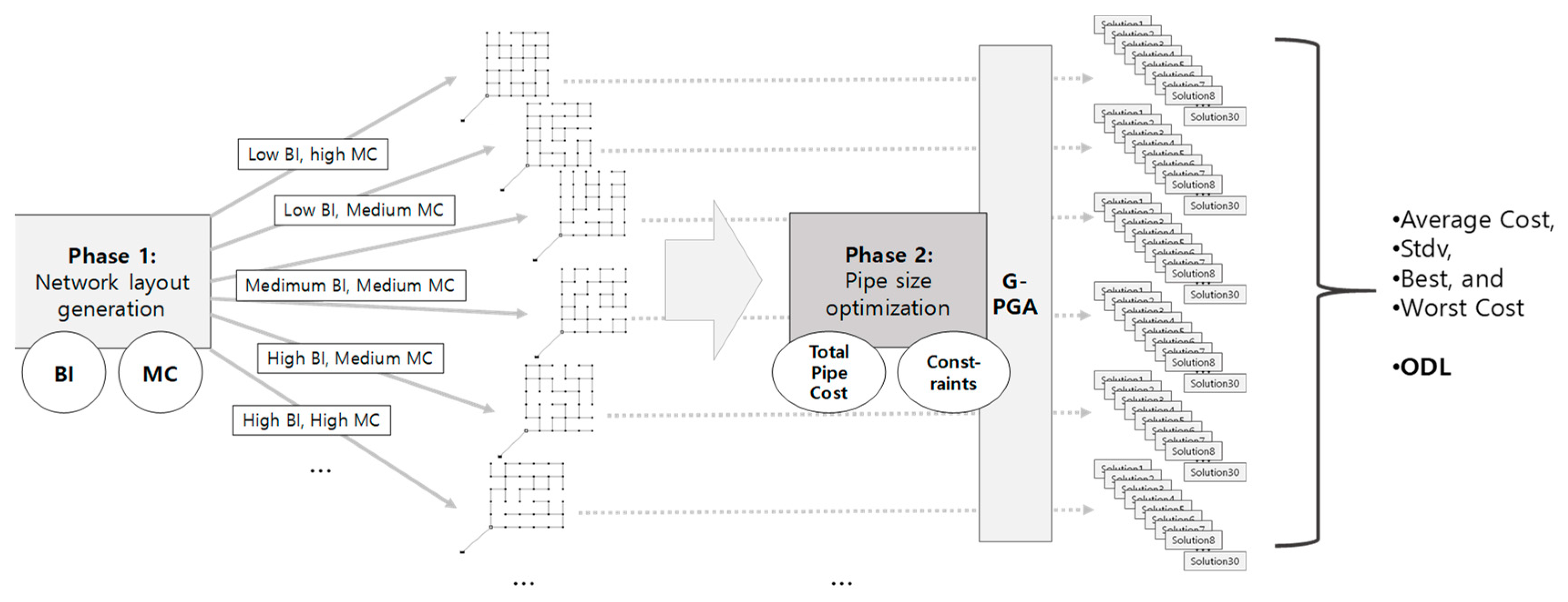
In this study, an ODL indicator was developed: the coefficient of variation (CV) of the final solution costs. The ODL quantified the degree of optimization difficulty, and the indicator was applied to WDNs of various characteristics to provide guidelines on WDN design. An ODL quantification framework was also developed with two phases: (1) generating network layouts with various topological characteristics, and (2) quantifying the statistics of the final solution quality and ODL by using a global parallel genetic algorithm (G-PGA). Two topological measures were used to generate networks with distinctly different layouts in Phase 1: a branched index (BI) and meshedness coefficient (MC). In Phase 2, the G-PGA was used in 30 independent optimization trials to obtain the statistics of the final solution quality and ODL. The proposed indicator and two-phase framework were applied to the design of a dense-grid B-city network and large dense-grid C network to test attribution of network scale to the ODL. A series of computational experiments were performed to identify the system characteristics and optimization conditions affecting the ODL.

2. Methodology

Here, the proposed ODL indicator is described along with other final solution quality indicators used to investigate the factors that affect the convergence of WDN optimal design solutions. The numerical optimization of the WDN design is performed in two phases: (1) layout generation and (2) pipe size optimization. The details of the two phases, including two topological indicators and the network classification method, are also described, as well as statistical measures. Finally, the warm initial approach is presented. All of the simulations were performed using MATLAB, and EPANET 2.0 was used for hydraulic analysis, which was executed using the MATLAB EPANET toolkit.

2.1. Optimization Difficulty Level

The global optimum is easily and consistently found in a simple optimization problem. For example, Kim et al. [25] found the global optimum of a two-dimensional mathematical benchmark optimization problem every time in 100 independent optimization trials with five out of six MOAs. The global optimal solution to the cost of the pipe sizing problem for the Hanoi network (32 nodes and 34 pipes) [26] is known to be 6.081 million USD [10]. Different algorithms and optimization trials have yielded less than a 1% difference in solution cost compared to the global optimum [10,27]. However, such a difference generally increases with the problem size and complexity.

The proposed ODL indicator considers the variance of the final solution costs to quantify the ODL of a WDN. A high variance indicates that it is difficult for an MOA to find a converged global optimal solution. However, these variations tend to increase with network size and average solution cost. Therefore, the variance (or standard deviation) is normalized by the average solution cost. The proposed ODL indicator is calculated as the CV of solution costs obtained from a set of independent optimization trials:

$$\mathrm{ODL}=\frac{\sigma \left(FS{C}_i\right)}{\overline{FSC}} i = 1, 2, \dots , n$$

(1)

where $FS{C}_i$ is the final solution cost of the ith optimization trial, n is the total number of optimization trials, $\sigma$() is the standard deviation calculator, and $\overline{FSC}$ is the averaged final solution cost computed from the results of n optimizations. In order to calculate the ODL, the same number of function evaluations should be allowed for each of the n optimization trials.

The proposed ODL indicator compares the ODLs of WDNs. Thus, the same MOA should be used consistently for a set of networks to remove the potential effects of different MOAs being used. Note that four final solution quality measures (i.e., best, worst, and average solutions with their variance) are generally quantified and compared comprehensively when comparing MOA performances with a WDN. However, these often cannot be used to clearly conclude if an MOA offers superior performance (e.g., [10,11]).

2.2. Two-Phase ODL Examination Framework

To quantify and compare the ODLs of WDNs, an ODL examination framework is proposed with two phases: (1) layout generation and (2) WDN design optimization (Figure 1). In Phase 1, a set of layouts with different degrees of branchedness and loop density is generated from a grid network. In Phase 2, WDN optimal designs are sought with randomly generated solutions to the layouts to compute the statistics for the final solution quality.

2.2.1. Phase 1: Layout Generation

The network topology can be defined by network graph measures such as the BI, MC, and average node degree [28,29]. Phase 1 employs the BI and MC. Hwang and Lansey [28] developed a decision-tree-like WDN classifier where a WDN is classified into either (1) transmission branches and loops or (2) distribution branch hybrids and grids. Each branch of the tree is determined with respect to the network’s BI and MC values. The aim of Phase 1 is to yield a set of network layouts with distinctively and significantly different network topological characteristics.

Branch Index

The BI is the ratio of branched edges to the number of branched edges plus the number of edges in a network [28]:

$$\mathrm{BI}=\frac{e_b}{e+e_b}$$

(2)

where e and e_b denote the numbers of edges and branched edges, respectively. A branched edge means that it is not located in a loop. A larger BI corresponds to a more branched network. Hwang and Lansey [28] classified a WDN with a BI ≥ 0.5 as a branched network; otherwise, the network is identified as gridded, a hybrid (a mix between branch and grid layouts), or looped.

Meshedness Coefficient

The MC measures the connectivity of a WDN by comparing the number of cycles (loops) with the potential maximum number of cycles [30]. A larger MC corresponds to a more connected network with a higher loop density. The MC is computed as

$$\mathrm{MC}=\frac{e-n+1}{2n-5}$$

(3)

where n is the number of nodes in a network. The MC has been used as a redundancy measure to capture the degree of looping in a WDS [28,29,31,32]. Hwang and Lansey [28] considered looped networks as dense if MC > 0.2 and sparse otherwise.

Layout Generation Model

A network layout with predefined BI and MC values is found with the layout generation model, which minimizes the sum of penalty functions (F₁):

$$\mathrm{Minimize}{F}_1=\left|{\mathrm{BI}}_{target}-{\mathrm{BI}}_i\right|P_{BI}+\left|{\mathrm{MC}}_{target}-{\mathrm{MC}}_i\right|P_{MC}+N_{disconnected}{P}_{disconnected}$$

(4)

where BI_target and MC_target are the target BI and MC values, respectively; BI_i and MC_i are the ith layout solution’s BI and MC values, respectively; P_BI and P_MC are the penalty factors considered for BI and MC, respectively, which are assigned based on the target BI and MC values; N_disconnected is the disconnection degree calculated by ${\displaystyle \sum }_{j = 1}^{n}b$, where b = 0 if the jth node is connected to water source (i.e., a reservoir) and b = 1 otherwise (j = 1, 2, …, n); and P_disconnected is the penalty factor of the disconnection, which generally requires a relatively large value (e.g., more than 10,000) to prevent any disconnection in the network. The layout generation model seeks a feasible optimal layout with no penalty values (i.e., F₁ = 0) for BI_target and MC_target. Note that the pipe sizes are not determined in Phase 1; only pipe installation (whether or not to install a pipe at a link) is determined at each link. During the network generation and BI and MC calculations, a node-reduction algorithm [28] is used to remove nodes along a single pipe that do not affect the network structure and cause errors in the structural measure calculations. A thorough analysis might be needed for the penalty factors given to Equation (4).

Various network layouts with different sets of BI and MC values are found by changing the BI_target and MC_target. These are then input in Phase 2 to find the optimal pipe sizes for the layouts in Phase 1 (Figure 1).

2.2.2. Phase 2: WDN Design Optimization

Pipe Size Optimization Model

In Phase 2, the least-cost solution of a pipe sizing problem is identified for the layouts generated in Phase 1 (Figure 1). Therefore, the objective in Phase 2 is to minimize the total pipe cost given a network layout (L):

$$\mathrm{Minimize}{F}_2={\displaystyle \sum }_{k = 1}^l(Unitcos{t}_k\times {\mathrm{L}}_k|L_{\mathit{i}})$$

(5)

$$\mathrm{Subject}\mathrm{to}{P}_j\ge P_{min} j = 1, 2, \dots , n$$

(6)

where Unitcost_k and L_k are the unit pipe cost and length of pipe k (k = 1, 2, …, l), respectively; Li is a k × 1 binary matrix that indicates the pipe locations (pipe layout) of the ith solution and has the element of 1 at a pipe location and 0 otherwise (no pipe); P_j is the jth node’s pressure; and P_min is the minimum allowable pressure. The unit pipe cost is calculated by using the pipe construction cost function from [33]. The objective function and pressure constraint are consistently applied to the optimization of every layout, and a penalty is applied to the objective function if the constraint is violated.

Except for the case when the warm initial approach is used, independent optimization runs are begun with randomly generated initial solutions. Post-optimization analysis is performed to calculate the statistics of the final solution quality: the minimum, maximum, and average costs; standard deviation; and per pipe system cost (PPSC). The PPSC is computed by dividing the average cost by the total number of pipes l and is used to check its relationship with network structural measures. Finally, the ODL indicator is calculated by dividing the standard deviation by the average cost (Equation (1) and Figure 1).

Global Parallel Genetic Algorithm

Parallel computing is widely used in large-scale WDN optimization problems [34,35,36,37]. Because performing 30–50 optimization trials per layout is computationally very demanding, a GA based on parallel computing was used for optimization. In the domain of soft computing, global GA refers to a GA that distributes and evaluate its fitness calculations concurrently under different processors in a computer. On the other hand, non-global GAs are generally called grained GAs (coarse or fine-grained), which send subgroups of populations to each processor, who performs crossover and mutation on their own. In the migration period (e.g., every 1000 iterations), they share the best or worst solution in regards to search information.

In Phase 2, a G-PGA is used to seek optimal solutions for the WDN least-cost design problems given in Equations (5) and (6). The G-PGA distributes the most time-consuming task (i.e., fitness evaluations) to multiple parallel processors and reduces the central processing unit (CPU) computation time by 1/NP × 100%, where NP is the number of parallel processors that simultaneously perform the calculations [38]. Parallelization can be performed either within a single machine simultaneously using processors in a CPU/graphics processing unit (GPU) [20,39,40,41], or with a group of connected machines (e.g., distributed/cloud computing) (e.g., [42,43]). Note that a within-a-machine parallelization scheme was used in this study. The crossover and mutation of the G-PGA are performed in the host processor based on the fitness values evaluated by multiple slave processors. A penalty cost is added to the total pipe construction cost (Equation (5)) to handle constraints so that infeasible solutions are naturally excluded from the population.

2.3. Warm Initial Solution Approach

Randomly generated (i.e., cold) solutions can benefit the early optimization of a MOA because each solution’s starting point is scattered throughout the solution space, which increases the search diversity. However, the random initial solution is a poor approach to engineering problems with respect to feasibility and reasonability. With a random solution, upstream pipes can be much smaller than downstream pipes, and an irregular pipe size hierarchy is often used (e.g., non-smooth pipe changes such as 500 → 1000 → 300 mm). To overcome this limitation, Kang and Lansey [44] introduced a warm initial solution approach that generates a WDN pipe set with high engineering feasibility that satisfies pipe flow velocity constraints. In contrast to the cold solution, the warm solution is a mature and engineering-feasible solution that is believed to be close to the global optimal solution.

Kang and Lansey’s [44] warm initial approach consists of a series of steps and is briefly described here. First, the smallest pipe size (e.g., 50 mm if the available pipe set is 50, 100, 200, …, 1000 mm) is set to every pipe; then, the network hydraulics are calculated under this condition with EPANET [45]. Second, the pipe diameter is increased to the next-smallest size (e.g., from 50 to 100 mm) for a pipe whose velocity is higher than the predefined velocity constraint (e.g., 0.914 m/s (3 ft/s)). The above steps continue until all pipes have a velocity smaller than the constraint. As the steps are repeated, the network receives large pipes upstream and small pipes downstream. The effectiveness of the warm initial approach at obtaining engineering-sound final solutions was verified by [44] and [46]. The present study focused on investigating its impact on the final solution convergence.

2.4. Study Network

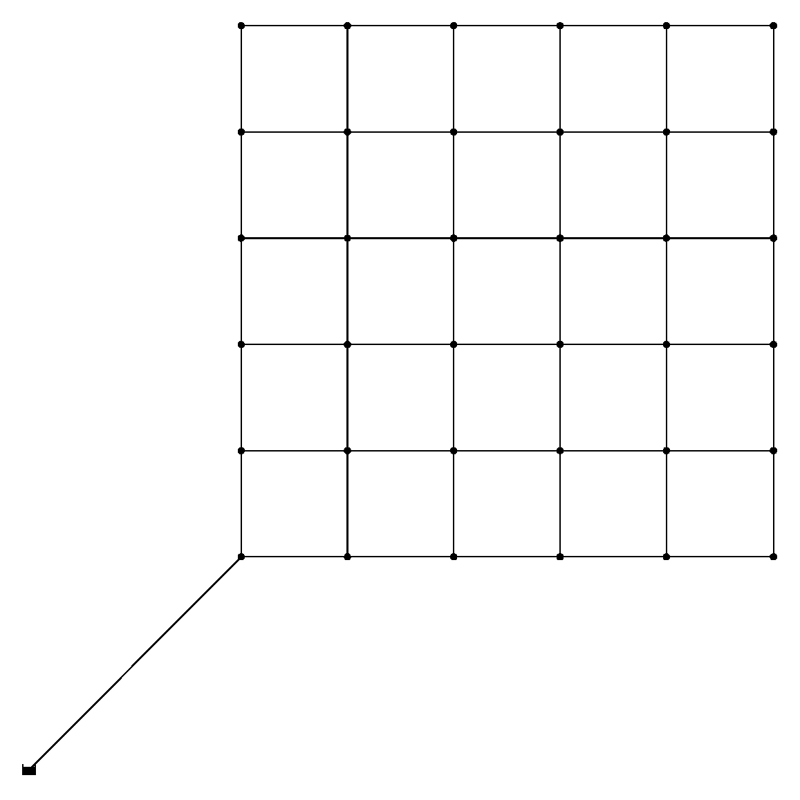
The above methodologies were applied to the B-city network [20], which consists of 36 nodes and 61 pipes (Figure 2). The total source reservoir head is 80 m (262.5 ft). The B-city network has 2 × 2 km (1.24 × 1.24 mi) grids and consists of a districted residential area. The network needs to supply 3409.2 L/s (54,037 gpm) of water, and each node has a demand of 94.7 L/s (1501 gpm).

In order to test the trend of the ODL to the scale of the network, the ODL and two topological measures were analyzed for the C network. The C network is a large, dense grid network that is an expanded version of the B-City network toward north and east directions. Therefore, 4 × 4 km (2.48 mi × 2.48 mi) grids are included in the C network. The total system demand is 13,636.8 L/s (0.216 Mgpm), while each nodal demand is identical to that of the B-City network. In this study, the reservoir head was increased to 117.7 m (386.2 ft).

The network classification scheme proposed by Hwang and Lansey [28] was employed to classify the topology of the B-City network. Note that the BI and MC of the full B-City network and C network (i.e., with a pipe at every link) were computed to be 0.02 and 0.424 for the B-City network, respectively, and 0.003 and 0.44 for C network, respectively, indicating that the both networks’ topologies are a dense grid. The original topologies of both networks were then modified as branched or sparse grids in Phase 1 (Figure 1).

For pipe size optimization in Phase 2, pipe sizes were selected from 16 available commercial pipe sizes with corresponding unit costs (

Table 1. Available commercial pipe sizes and corresponding unit costs.

Pipe Size (mm)	Unit Cost (USD/m)	Pipe Size (mm)	Unit Cost (USD/m)
50	86.3	800	873.6
100	95.2	900	1230.1
200	117.1	1000	1698.8
300	150.6	1200	3049
400	204.6	1400	5098.9
500	290.2	1600	8043.4
600	420.4	1800	12,091.5
700	609.5	2000	17,469.2

). The unit costs were calculated with the pipe construction cost formula proposed by [33] and parameters used by [47]. The minimum allowable pressure was 28.1 m (40 psi). The Hazen–Williams roughness coefficient was 120 for all pipes. Hydraulic simulations were performed with EPANET to check the pressure constraints. Multipoint crossover and regular mutation were performed with probabilities of 85% and 5%, respectively, in the G-PGA. A population of 100 was divided among four multiple processors (25 solutions each), and their fitness values were quantified concurrently.

3. Application Results

3.1. Optimization Difficulty Level and Two Topological Measures

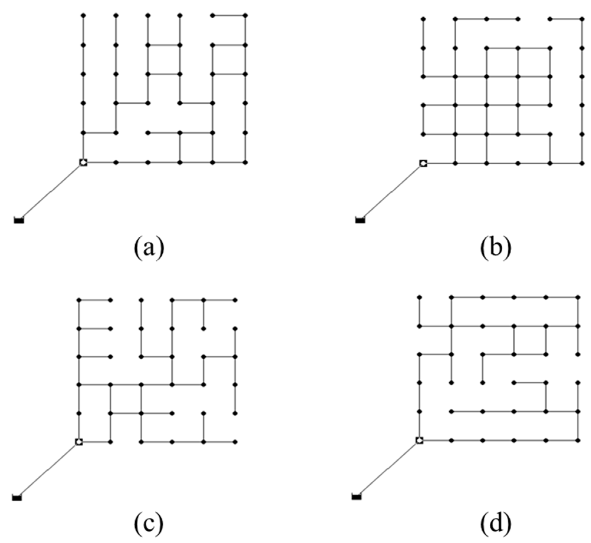
In order to identify any correlation between the ODL and two WDN topological measures, 25 pipe layouts were generated with a range of BIs and MCs. The measures were discretized, and each combination was assigned to a pipe layout. For example, the BI was discretized to 0.02, 0.1, 0.2, 0.4, 0.6, 0.77, 0.85, 1.0, and so on, whereas the MC was discretized to 0.0, 0.1, 0.16, 0.2, 0.3, 0.4, and so on. Hwang and Lansey [28] classified a WDN as branched when BI ≥ 0.5 and looped if not. They considered MC = 0.2 as the critical value for whether a network is dense or sparse. In total, 30 independent design optimizations were performed, beginning from identical sets of randomly generated solutions for a fair comparison of different pipe layouts. 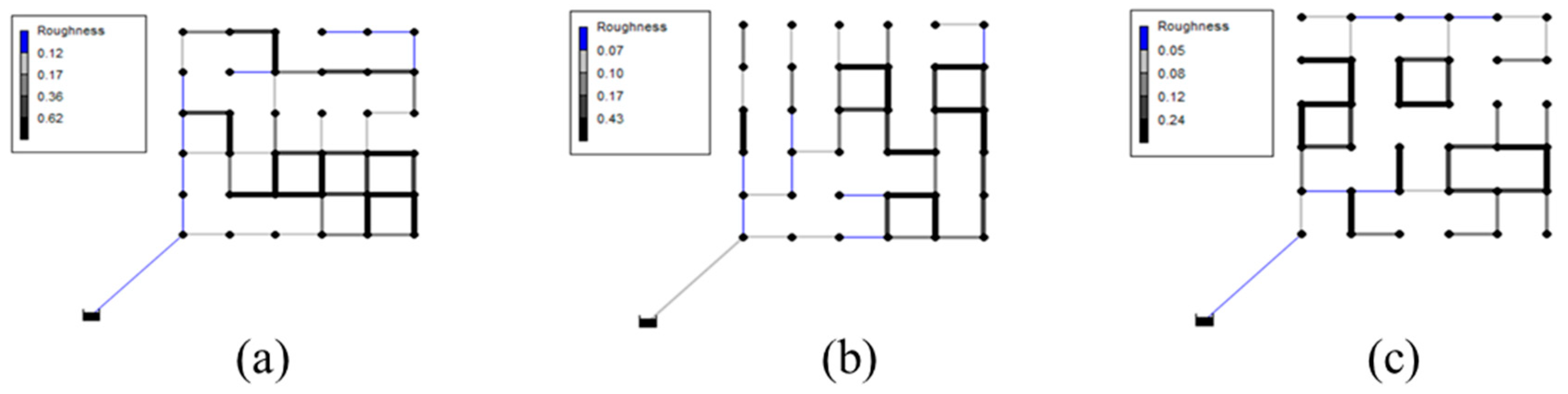Figure 3 shows some of the pipe layouts generated in Phase 1 that were used for the numerical experiments.

The average of the absolute error between target and optimized topological measures (e.g., $\left|{\mathrm{BI}}_{target}-{\mathrm{BI}}_i\right|$ and $\left|{\mathrm{MC}}_{target}-{\mathrm{MC}}_i\right|$ in Equation (4)) was obtained from 100 independent Phase 1 optimization runs with a range of the penalty factors P_BI and P_MC (Equation (4)) and summarized in

Table 2. Averaged absolute errors of the branch index (BI) for different penalty factors.

		PBI
		100	101	102	103	104	105
PMC	100	0.119	0.106	0.102	0.102	0.103	0.105
	101	0.217	0.117	0.104	0.102	0.101	0.101
	102	0.265	0.213	0.114	0.099	0.103	0.104
	103	0.266	0.267	0.210	0.115	0.101	0.104
	104	0.276	0.264	0.266	0.213	0.117	0.105
	105	0.271	0.261	0.268	0.264	0.213	0.117

and

Table 3. Averaged absolute errors of the meshedness coefficient (MC) for different penalty factors.

		PBI
		100	101	102	103	104	105
PMC	100	0.085	0.116	0.121	0.121	0.122	0.129
	101	0.053	0.085	0.116	0.120	0.123	0.124
	102	0.051	0.054	0.084	0.119	0.122	0.117
	103	0.052	0.051	0.052	0.085	0.114	0.119
	104	0.052	0.051	0.052	0.054	0.084	0.116
	105	0.051	0.051	0.052	0.052	0.054	0.087

for the BI’s and MC’s sensitivities, respectively. As shown in both tables, absolute error tends to decrease when the higher penalty factor is assigned for each topological measure (right-up for BI (Table 2) and left-down for MC (Table 3)). Multiplying a higher penalty factor assigns greater weighting to the topological measure in the objective function F₁ in Equation (4). Therefore, the minimum absolute error overall could be obtained in cases where the two penalty factors P_BI and P_MC were identical (diagonal in Table 2 and Table 3). In this study, the P_BI and P_MC of 10⁵ are used in Equation (4).

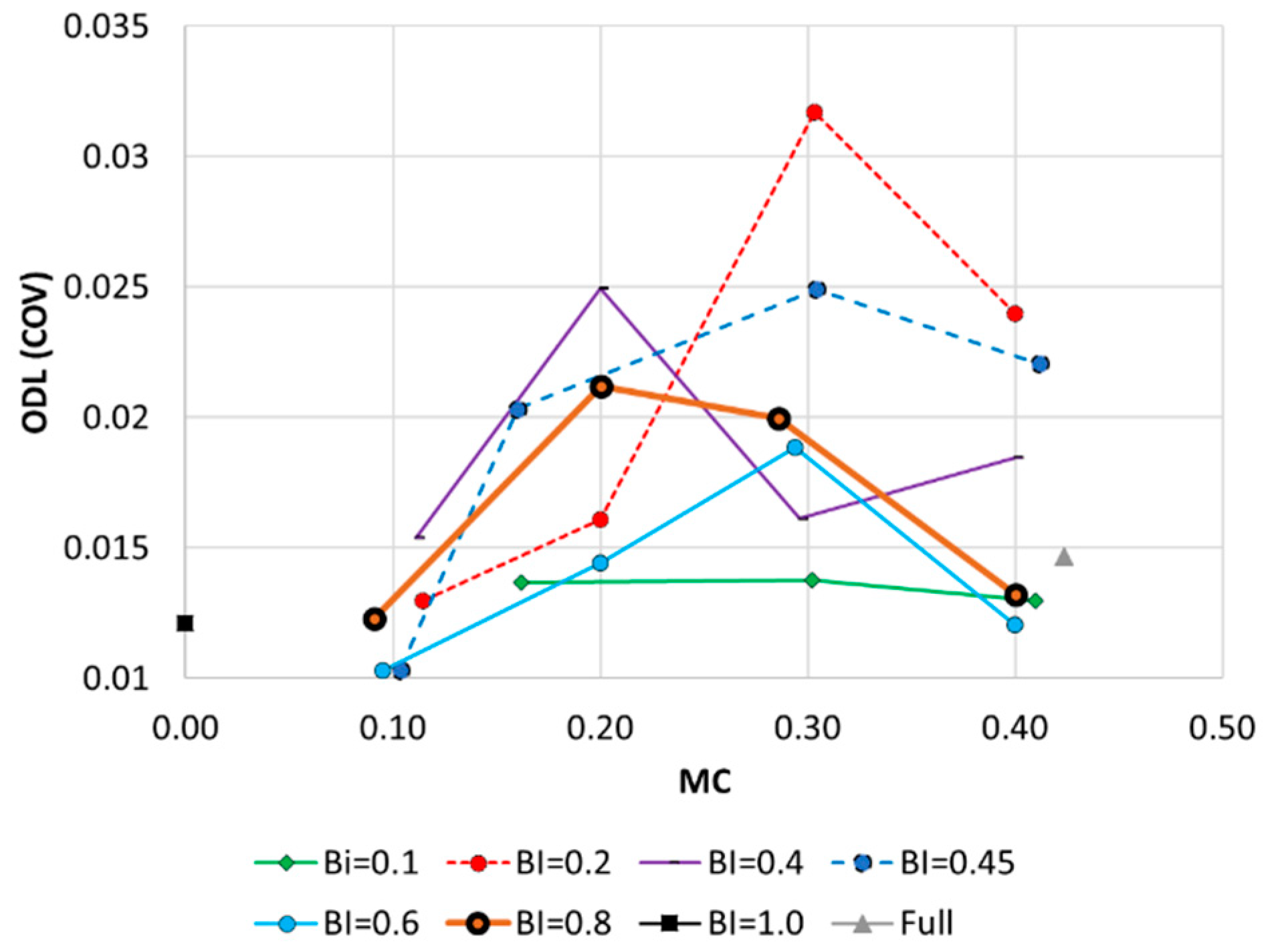
Figure 4 shows the ODLs of the 25 networks. A high ODL indicates that converging to a global optimal solution for the layout was difficult. For reference, the ODL of the full network with a pipe at all links was quantified and is plotted in Figure 4 (gray triangles). The optimization difficulty was also estimated for a perfectly branched layout as another reference point (i.e., BI = 1.0, MC = 0.0) (black rectangles). Each plot represents the ODL values for a range of MCs in the networks with the same BI.

Although some stochastic patterns were observed, a concave plot was commonly obtained regardless of the network’s BI. The highest ODL value was observed at MC = 0.2–0.3, and low- and high-MC networks (i.e., MC = 0.1 or 0.4) had low ODL values. For example, in networks where the BI = 0.8, the ODL increased from 0.0123 at MC = 0.09 to 0.0212 at MC = 0.2 (72.4% increase), while it decreased from 0.02 at MC = 0.29 to 0.0132 at MC = 0.4 (34% decrease). Therefore, the ODL was highest in medium-meshed (medium-dense) networks with a mixture of branches and loops. An overly dense network has a relatively low ODL (Figure 4).

According to the denominator of Equation (1), the averaged cost $\overline{FSC}$ increases with the MC and number of pipes (toward the right-hand side of the MC axis in Figure 4). The concave change in ODL values indicates that the standard deviation (or variance) of the final solution cost has a more significant concave change with respect to changes in the network MC (Figure 4).

Figure 5 shows the variance in pipe diameters at each pipe of the final solutions for different layouts with different sets of BIs and MCs. A high diameter variation (thick pipes in Figure 5) was identified at downstream looped pipes, while transmission lines near the source had low diameter variations. Considering the large diameter (and high cost) of transmission lines, this small variation indicates that local looped pipes have a significant influence on the total system’s ODL.

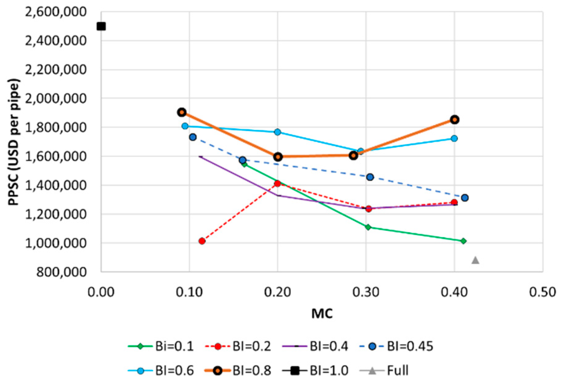
The experimental results confirmed that, as the MC increases, the PPSC decreases in looped networks (BI < 0.8). For example, more unit loops (i.e., a loop equivalent to a single grid (Figure 2)) are included in high-MC low-BI networks (e.g., Figure 3b). Adding more small and low-cost pipes increases WDN redundancy, which can reduce overall pipe diameter, total system cost, and PPSC. Meanwhile, a highly branched network (BI = 0.8) shows convex PPSC changes with an increasing MC (Figure 6). Highly branched high-MC networks (BI > 0.8 and MC ≥ 0.3) have a combined large loop at the end of a branch line, which requires more investment in transmission lines near the source and thus increases the PPSC (e.g., Figure 3d).

3.2. Numerical Experiments on System Characteristics/Optimization Conditions

A series of computational experiments were performed to identify system characteristics and optimization conditions that affect the ODL. The following factors were considered: (1) elevation change (to check the impact of the elevation distribution on the ODL); (2) multiple reservoirs (to see if multiple water supply sources change the ODL); (3) source supply condition (to compare the ODLs of gravity-fed and pumped supplies); and (4) the warm initial solution (to investigate whether using a better initial population improves the search for an optimal solution). All searches began with a randomly generated initial population, except for when the warm initial solution was considered.

In order to derive generalized conclusions, four networks out of a total 25 layouts with different levels of network branchedness and density were selected: (1) a pipe at all links (full network), (2) BI = 0.2 and MC = 0.3, (3) BI = 0.81 and MC = 0.29, and (4) BI = 1.0 and MC = 0. While Networks 1 and 4 had the maximum and minimum network densities, respectively, Networks 2 and 3 had low and high branchedness, respectively. The CV of the system costs of the final solutions was calculated for each case from a total of 30 independent optimization trials.

3.3. Elevation Change

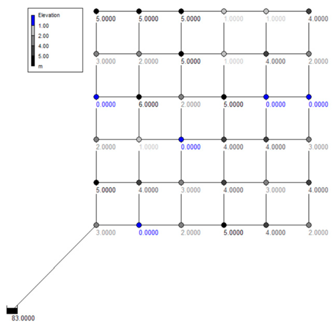
The impact of nodal elevation heterogeneity on the ODL was investigated. Three elevation distribution cases were generated with the four selected layouts: plane elevation (Case 1), consistently increasing elevation (Case 2), and random elevation (Case 3). The nodal elevation was 0 m at all nodes in Case 1. In Case 2, the elevation increased incrementally from 0 m at the node immediately downstream of the single source, to 6 m at the node in the northeastern corner of the network (Figure 2). In Case 3, nodal elevations were randomly selected among the integers of 0–6 (Figure 7).

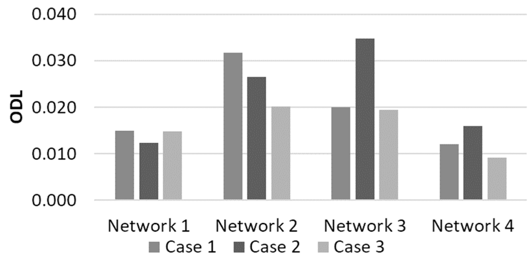
Figure 8 shows the ODL obtained for the four selected layouts under the three nodal elevation conditions. The ODL was highest with a consistently increasing elevation (Case 2) for the branched networks (Networks 3 and 4). On the other hand, the ODL was highest with a plane elevation (Case 1) for the dense networks (Networks 1 and 2). The overall ODL was confirmed to increase from Networks 1 to 2 and 3 (from dense to branched networks) and decrease from Networks 3 to 4 (from branched to skeletonized networks). Contrary to expectations, Case 3 had the smallest overall ODL of most networks (Figure 8). This may be because finding an optimal design solution is difficult when hydraulic continuity and dependency exist within a network. There should be smooth pipe diameter changes in a layout when a smooth elevation change is present, where the diameters of the upstream and downstream pipes are determined according to their dependency. Infeasible solutions from MOA operations (e.g., crossover and mutation in GA) are more likely to be generated under the above condition. However, pipe sizes of a local sub-grid would not be highly dependent on the other side of a network with random elevations.

3.4. Multiple Reservoirs

Supplying water from multiple reservoirs complicates the hydraulics of a WDN. Although the overall network redundancy improves as alternative water supply paths increase, the pipe flow and pressure distributions change even with minor system changes (e.g., pipe diameter changes, demand fluctuations) when there are multiple reservoirs. Another reservoir was added to the northeastern end (Figure 2) of each of the four selected layouts. Note that Networks 2–4 were generated under the single-reservoir condition.

Table 4. ODL and PPSC obtained under the single- and two-reservoir supply conditions.

Reservoir	Indicator	Network 1 (Full Network)	Network 2 (BI = 0.2, MC = 0.3)	Network 3 (BI = 0.81, MC = 0.29	Network 4 (BI = 1.0, MC = 0)
Single reservoir	ODL	0.0147	0.0317	0.0200	0.0121
	PPSC (M USD/pipe)	0.88	1.24	1.61	2.50
Two reservoirs	ODL	0.0239	0.0332	0.0577	0.0390
	PPSC (M USD/pipe)	0.77	1.13	2.55	1.05

summarizes the ODL and PPSC values obtained for the networks with one and two reservoirs. The ODL was confirmed to be higher with two reservoirs than with a single reservoir. For example, the ODL of Network 3 was 188.5% higher with two reservoirs than with a single reservoir. This indicates that elaborate fine-tuning of the pipe diameter set is required when pipe flows and pressures are affected by multiple reservoirs. However, this often fails to minimize total costs and satisfy system governing equations (e.g., conservation of energy) and associated pressure constraints (Equation (6)).

Except for Network 3, the PPSCs were higher with a single reservoir than with two reservoirs (Table 4). This is because the distance of water supply paths from a source to a demand node obviously decreased with two reservoirs, which lowered the overall head losses through the paths and allowed for smaller pipe sizes.

3.5. Source Supply Condition

In a hydraulic model, a reservoir is assumed to have a constant water head and provide constant energy to the system. However, many real-world WDNs are supplied by a pumping station that provides different amounts of total energy depending on the total water inflow.

The most uncertain and dynamic parameter of a WDN is water demand [48]. In the last two decades, the stochastic nature of demand has been considered in research on WDN design by random demand sampling using either Gaussian or log-normal distributions with the base demand as the mean and an assumed CV (e.g., CV = 0.1) [47,49,50].

The changes to the ODL were examined when a fixed-head reservoir is replaced with a reservoir and pump station whose hydraulic behavior is defined by a pump characteristic curve. The pump curve was set to provide the same total head at the best efficiency point (BEP) as the reservoir-only condition, and the pipe diameter sets (i.e., design alternatives) needed to satisfy the pressure constraints under three different demand loading conditions: the base demand of previous examinations, and 90% and 110% of the base demand.

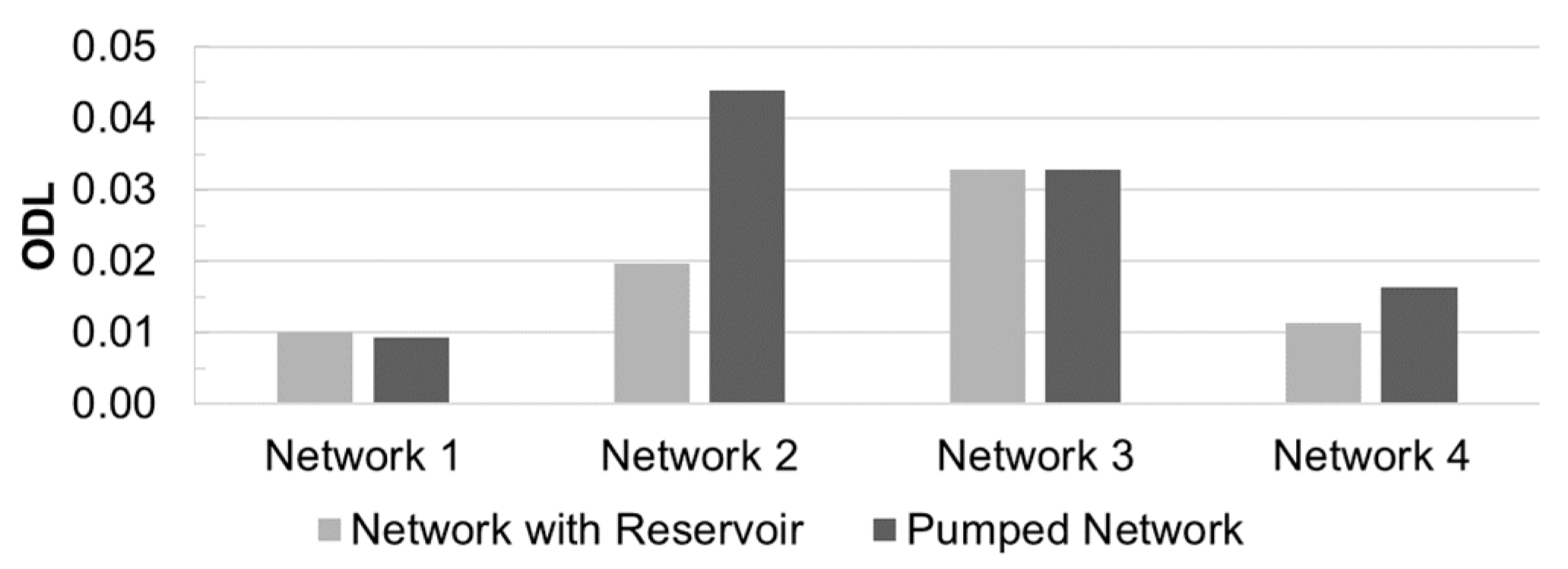
Figure 9 shows the ODL values obtained under the gravity-fed and pumped water supply conditions. While the ODL of the pumped system was greater than or almost equal to that of the fixed-head system (Figure 9), the highest ODL was observed for a dense network—Network 2 with a pump station (BI = 0.2 and MC = 0.3). The ODL was lowest for Network 1, which had full pipe density and the lowest branchedness.

3.6. Warm Initial Solutions

Finally, the impact of using warm initial solutions was investigated using two cases: (1) beginning the search with randomly generated solutions, and (2) using warm initial solutions that were generated according to the work done by [44]. The initial populations were independently generated in Case 1, and a single warm initial solution obtained from Kang and Lansey’s approach was seeded in the population in Case 2, while others were randomly generated as in Case 1. Slightly different velocity constraints (selected from discretized velocities ranging from 0.610 m/s (2 ft/s) to 1.219 m/s (4 ft/s)) were applied for each run.

Contrary to expectations, providing the seed solution (i.e., a similar starting point for different runs) did not affect the final solution’s convergence. It was not possible to derive a consistent conclusion from the comparison of the two cases (i.e., different cases had a higher ODL for each network layout). The percentage difference between the two cases of Networks 1 and 4 (a full and a perfectly branched network, respectively) was marginal, at about 10%, while that of the other networks was about 40%. Although using the warm initial solution approach results in more engineering-sound pipe sizes, the quality of the final solutions (i.e., closeness to the global optimum) relies more on the algorithm’s performance during the search than the starting point [18].

3.7. Combined Effect Investigation

Given the system factors identified in the previous sections, an interesting question is how the ODL of the network changes when different factors are combined. A reasonable assumption is that including more complicated system components and conditions increases the difficulty of finding the global optimum of the WDN. The ODL of the study network with two reservoirs (high ODL in the case of multiple reservoirs) and consistently increasing elevation (Case 2 and high ODL in the case of elevation change) was quantified to verify the assumption.

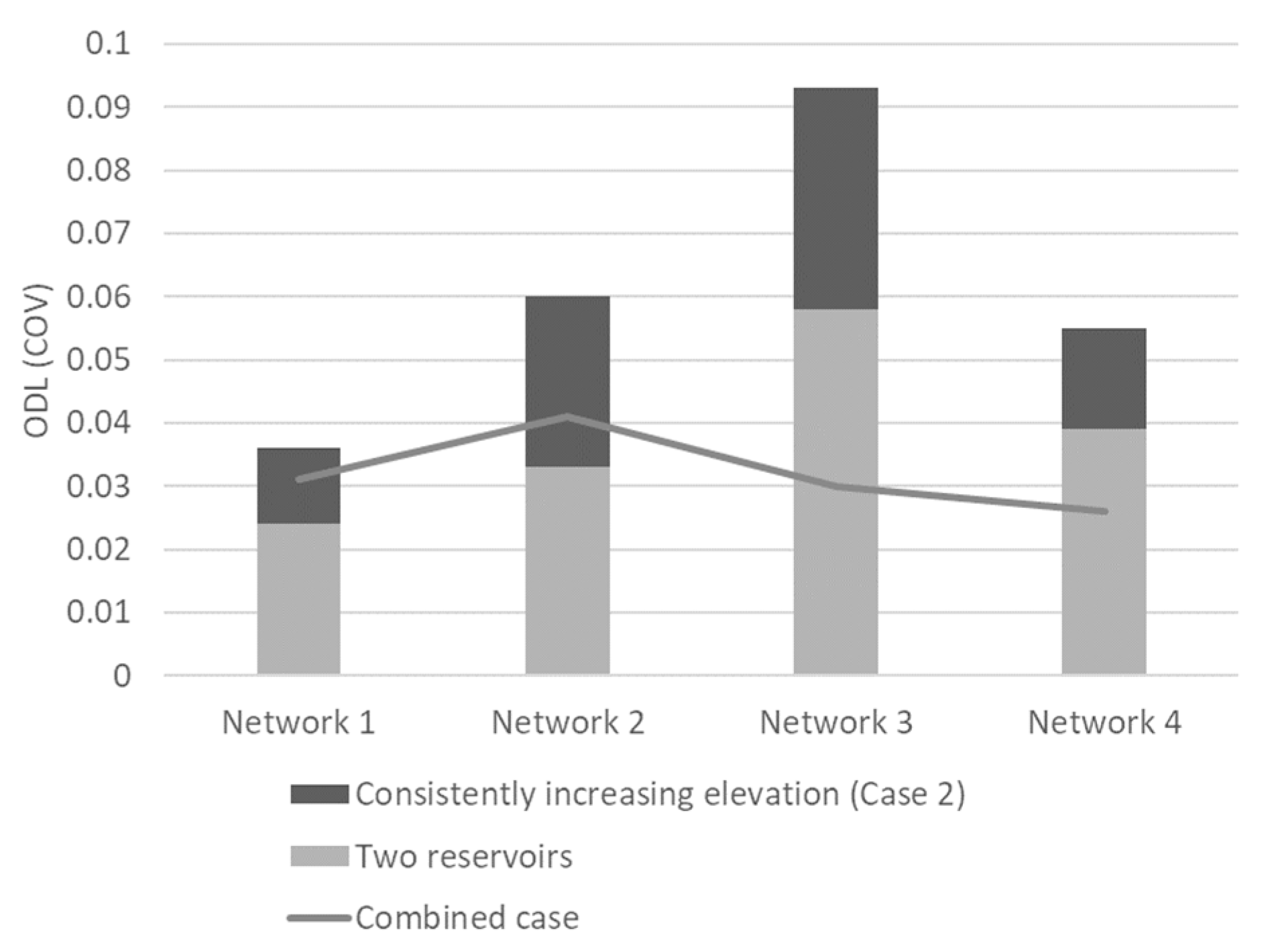
Figure 10 shows the ODL values of the final solutions for the four networks (Networks 1–4) with two reservoirs and consistently increasing elevation obtained from 30 independent optimization runs. Contrary to expectations, the ODLs were lower in the combined case than the sum of the ODLs in the network with individual changes (Figure 10). The gap between the two ODLs was highest for Network 3 with BI = 0.81 and MC = 0.29. For the branched networks (Networks 3 and 4), the ODL of the combined case was even lower than that of the network with two reservoirs. This confirms that the ODL cannot be computed according to the principle of superposition, and thus cannot be easily anticipated a priori. The system-wide hydraulic complexity determines the overall ODL. Therefore, preliminary optimization test runs should be performed with the proposed ODL indicator and two-phase examination framework to confirm the ODL of the problem of interest.

3.8. Testing in the Large C Network

In this section, the two-phase ODL processes were applied to the C network to check whether the conclusions made in the B-City network are consistently secured in a large network. A hundred independent design optimizations were performed in response to a large-scale problem. Other experimental conditions (e.g., layout derivation and pipe size optimization) were set identically to the previous demonstration. 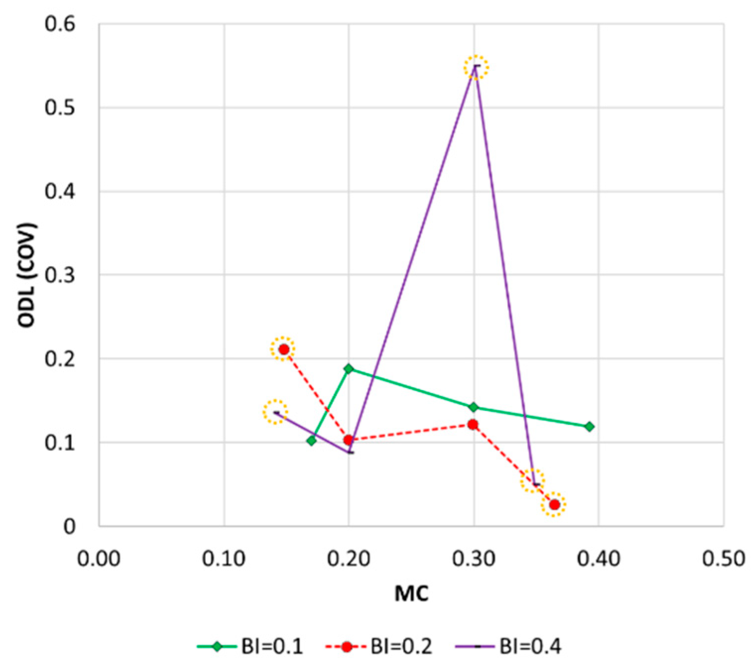Finally, the ODL value was computed from the optimal pipe diameter solutions obtained from 12 total layouts of each combination of BI = 0.1, 0.2, and 0.4 and MC = 0.1, 0.2, 0.3 and 0.4 (plotted in Figure 11).

First, the overall ODL values of the C network were higher than those of the B-City network, indicating that a large network is more difficult to optimize than a small/medium-size network. Note that, opposite to the B-City network, infeasible solutions were included in the solutions of the C network. All of 100 independent optimal solutions were feasible in the networks of BI = 0.1, while the resulting pattern of the curve was similar to that of the B-City network, a concave trend with the maximum ODL at MC = 0.2, 0.3 and low ODL at low- and high-MC. Although infeasible solutions were included within the 100 independent optimal solutions (marked as dashed circles in Figure 11), a similar concave pattern of the curve was identified in BI = 0.4.

The concave trend was not found when infeasible solutions were a majority of the optimal solutions (BI = 0.2). In summary, the ODL results of the C network verified that the ODL trend is concave regardless of network size, if feasible solutions are considered.

4. Summary and Conclusions

An ODL indicator was developed which is the CV of the final solution costs. An ODL quantification framework was also developed with two phases: (1) generating network layouts with various topological characteristics, and (2) quantifying the statistics of the final solution quality and ODL. Two topological measures were used in Phase 1: the BI and MC. Thirty independent optimization trials were performed in Phase 2 for each of the 25 layouts generated in Phase 1. A G-PGA was used for computationally demanding optimization tasks. The proposed indicator and quantification framework were applied to the design of a dense-grid B-City network and a large C network.

First, the relationship between the two topological measures (BI and MC) and ODL was investigated with the proposed framework. While a more distinct relationship was identified between the MC and ODL, the ODL was confirmed to be highest for medium-meshed networks and low for high- and low-MC networks regardless of network size. In addition, the ODL of the network was higher for the larger network. The pipe sizes did not easily converge at looped local parts of the study network. Overall, the PPSC decreased with an increasing MC because a high-MC network has looped subareas that increase the overall system redundancy and decrease the overall pipe size.

A set of numerical experiments was conducted to investigate the impact of system characteristics and optimization conditions on the ODL. Four cases were considered: (1) elevation change, (2) multiple reservoirs, (3) source supply condition, and (4) a warm initial solution. Four out of the total 25 layouts (with distinctly different sets of BI and MC values) that were considered in the previous experiment were used for this examination.

First, the optimal pipe set was sought for the four selected layouts with a plane elevation, consistently increasing elevation and random elevation. The smallest ODL was found for the network with random elevation because finding an optimal design solution is difficult when hydraulic continuity and dependency exist within a network (i.e., plane and consistently increasing elevation) for which infeasible solutions are easily generated. Second, the ODLs with one and two reservoirs were compared. The ODL was higher with two reservoirs than with a single reservoir. The PPSC increased for branched networks and was higher with a single reservoir than with two reservoirs.

Third, the ODL was quantified for the four selected networks under the gravity-fed and pumped supply conditions. The network hydraulic behavior was defined by a pump characteristic curve for the latter, while a consistent total head was supplied for the former. Regardless of the network layout, the ODL with the pump system was greater than or equal to that of the fixed-head system. Thus, dynamic hydraulic conditions hinder the convergence of optimal pipe size solutions. Fourth, the impact of using warm initial solutions on the ODL was investigated. Contrary to expectations, providing a warm initial solution did not affect the final solution’s convergence.

Finally, the combined effect of any two of the above system’s characteristic factors on the ODL was investigated. It was confirmed that considering additional changes to the system characteristics does not simply increase the ODL. The principle of superposition is not applicable to quantifying the ODL. Therefore, preliminary optimization test runs should be performed with the proposed ODL indicator and a two-phase framework to confirm the ODL of the problem of interest.

A feasible application for the proposed ODL would be utilizing an indicator for (1) comparing the effectiveness or efficiency of the selected MOA, and (2) identifying reliability of the final results. In addition, the proposed ODL indicator and two-phase framework could be used to test other WDN optimization problems such as pump and valve operation, large-scale planning problems, and selecting a proper MOA. Moreover, the ODL indicator could be used to generate a WDN benchmark problem with a target optimization difficulty, which is commonly applicable to testing new MOAs in the WDN domain. Finally, the proposed two-phase framework could be modified for different investigations and be extended to multi-objective optimization. Performance indices for multiple objectives should be used to quantify the ODL, such as the coverage set, diversity, and hypervolume.