Self-Adaptive Models for Water Distribution System Design Using Single-/Multi-Objective Optimization Approaches


Abstract
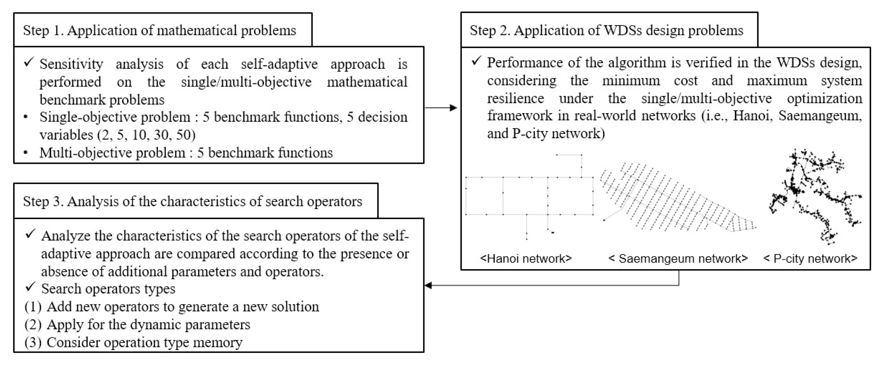
1. Introduction
- Addition of new operators to generate a new solution;
- Application of dynamic parameters (i.e., HMCR, PAR, and Bw) depending on number of iterations, harmony memory size, and decision variable (DV) size; and
- Consideration of the operation type in optimization process.
2. Optimal Design of Water Distribution Systems
2.1. Minimizing Construction Cost
2.2. Maximizing System Resilience
2.3. Hydraulic Constraints and the Penalty Function
3. Optimization Algorithms
3.1. Harmony Search
3.2. Parameter-Setting-Free Harmony Search
3.3. Almost-Parameter-Free Harmony Search
3.4. Novel Self-Adaptive Harmony Search
3.5. Self-Adaptive Global-Based Harmony Search Algorithm
3.6. Parameter Adaptive Harmony Search
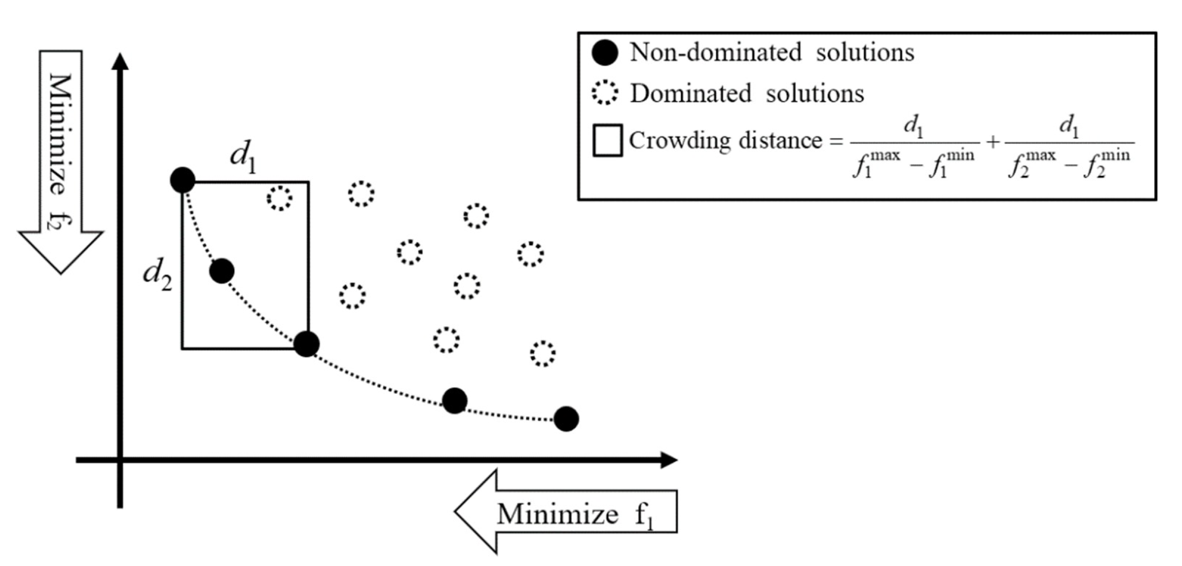
4. Multi-Objective Optimization Formulation
5. Application and Results
5.1. Performance Indices
5.2. Comparison of Algorithm Performance in Mathematical Benchmark Problems
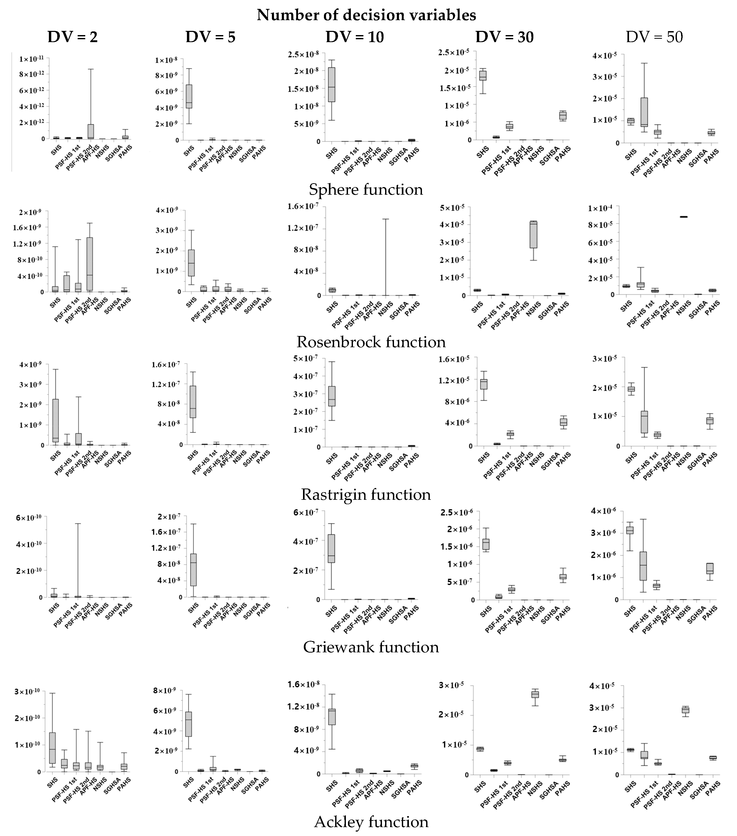
5.2.1. Single-Objective Optimization Problems
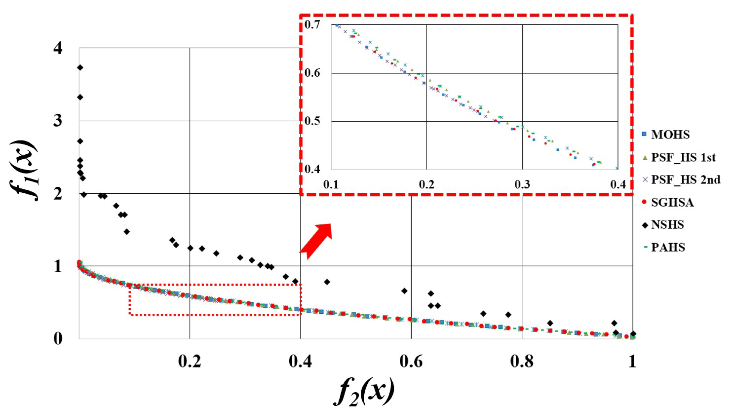
5.2.2. Multi-Objective Optimization Problems
5.3. Comparison of Self-Adaptive Technique Performance in WDS Design Problems
5.3.1. Single-Objective Optimal Design of WDSs
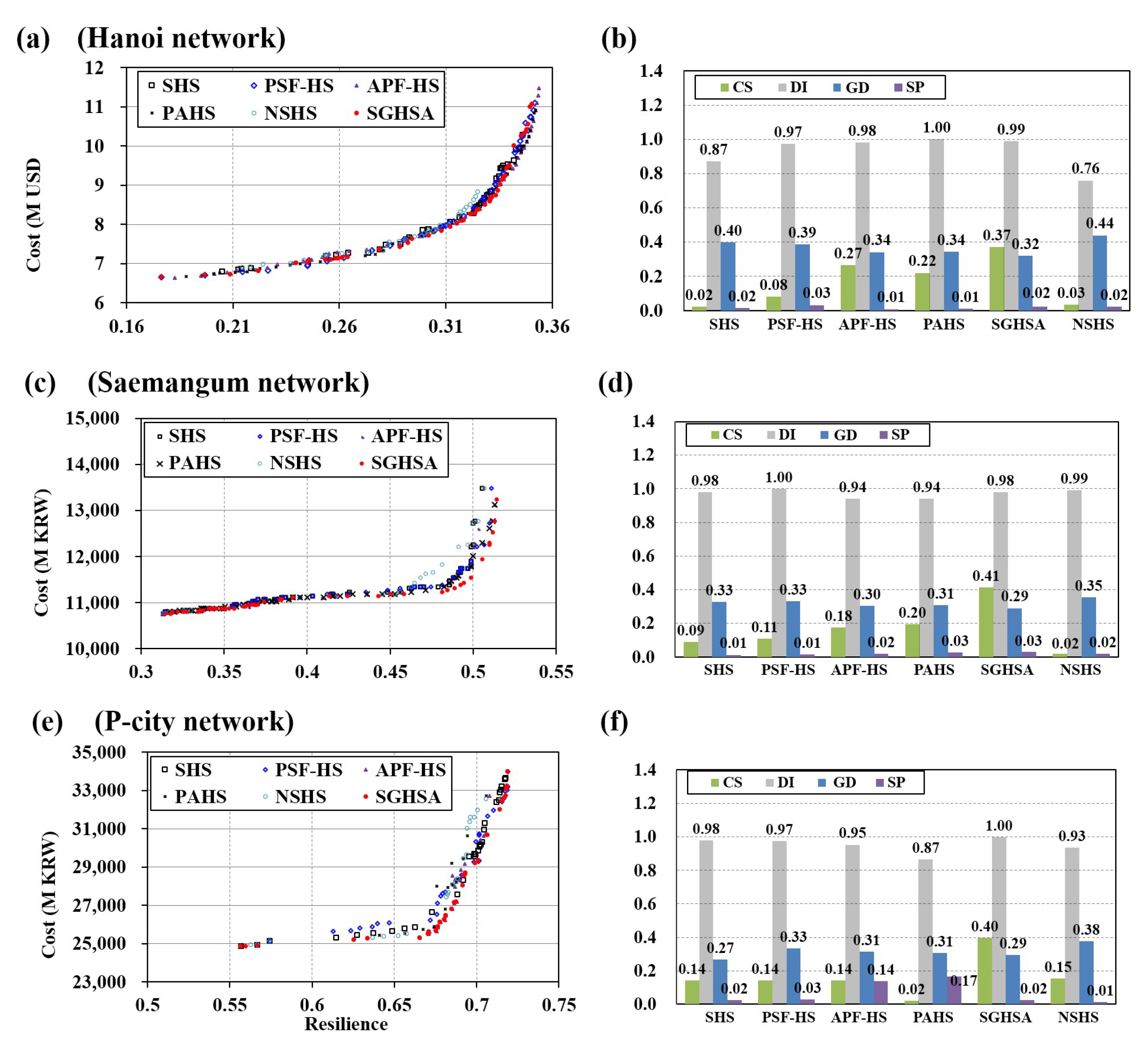
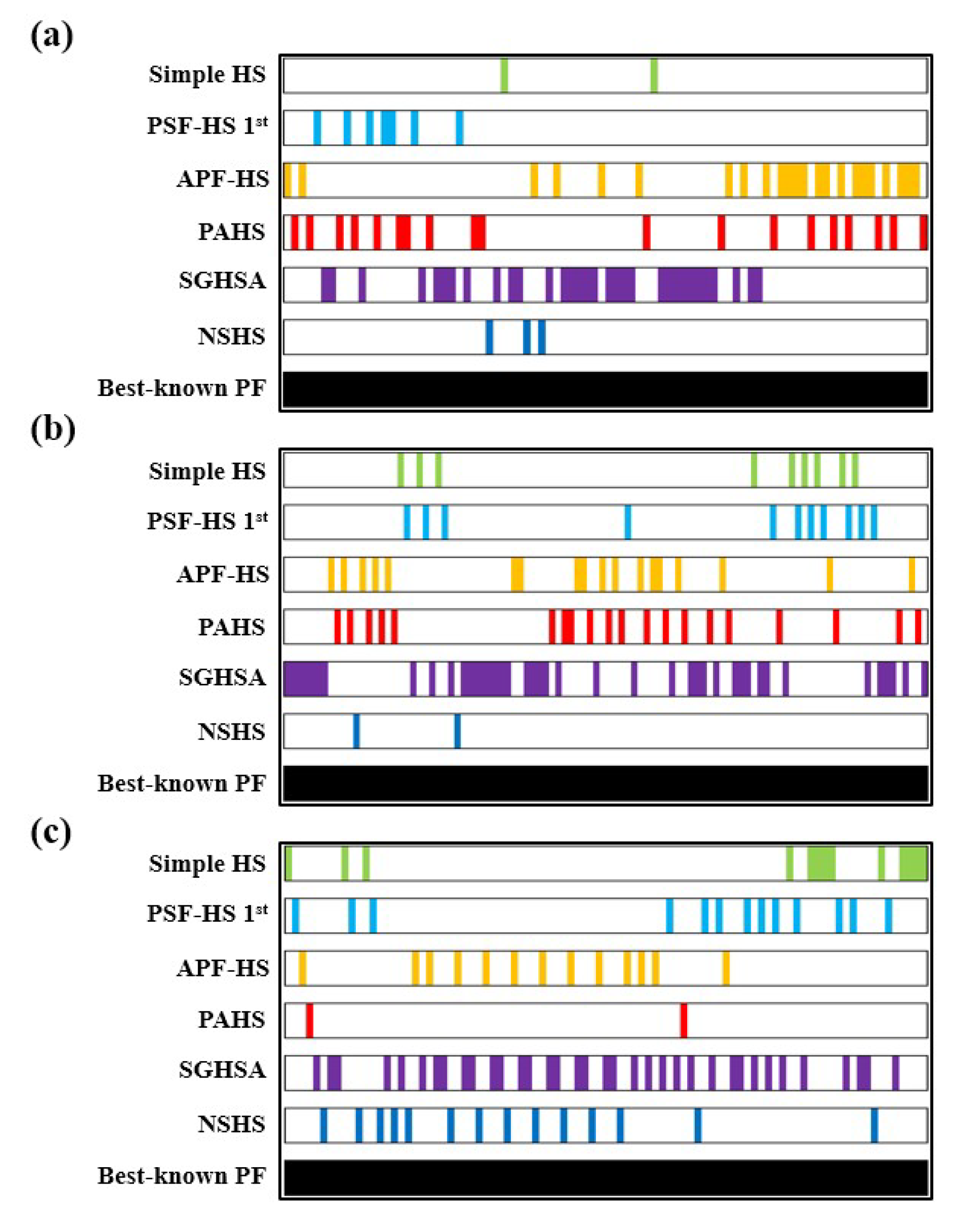
5.3.2. Multi-Objective Optimal Design of WDSs
5.4. Comparison of Algorithm Characteristics (i.e., Operator and Parameter)
6. Conclusions
Author Contributions
Funding
Acknowledgments
Conflicts of Interest
References
- Alperovits, E.; Shamir, U. Design of optimal water distribution systems. Water Resour. Res. 1977, 13, 885–900. [Google Scholar] [CrossRef]
- Quindry, G.E.; Liebman, J.C.; Brill, E.D. Optimization of looped water distribution systems. J. Environ. Eng. 1981, 107, 665–679. [Google Scholar]
- Goulter, I.C.; Coals, A.V. Quantitative approaches to reliability assessment in pipe networks. J. Transp. Eng. 1986, 112, 287–301. [Google Scholar] [CrossRef]
- Su, Y.C.; Mays, L.W.; Duan, N.; Lansey, K.E. Reliability-based optimization model for water distribution systems. J. Hydraul. Eng. 1987, 113, 1539–1556. [Google Scholar] [CrossRef]
- Kessler, A.; Shamir, U. Analysis of the linear programming gradient method for optimal design of water supply networks. Water Resour. Res. 1989, 25, 1469–1480. [Google Scholar] [CrossRef]
- Lansey, K.E.; Mays, L.W. Optimization model for water distribution system design. J. Hydraul. Eng. 1989, 115, 1401–1418. [Google Scholar] [CrossRef]
- Fujiwara, O.; Khang, D.B. A two-phase decomposition method for optimal design of looped water distribution networks. Water Resour. Res. 1990, 26, 539–549. [Google Scholar] [CrossRef]
- Schaake, J.C.; Lai, F.H. Linear Programming and Dynamic Programming Application to Water Distribution Network Design; MIT Hydrodynamics Laboratory: Cambridge, MA, USA, 1969. [Google Scholar]
- Wood, D. KYPipe Reference Manual. Civil Engineering Software Center; University of Kentucky: Lexington, KY, USA, 1995. [Google Scholar]
- Sherali, H.D. Global optimization of nonconvex polynomial programming problems having rational exponents. J. Glob. Optim. 1998, 12, 267–283. [Google Scholar] [CrossRef]
- Simpson, A.R.; Dandy, G.C.; Murphy, L.J. Genetic algorithms compared to other techniques for pipe optimization. J. Water Res. Plan. Manag. 1994, 120, 423–443. [Google Scholar] [CrossRef]
- Maier, H.R.; Simpson, A.R.; Zecchin, A.C.; Foong, W.K.; Phang, K.Y.; Seah, H.Y.; Tan, C.L. Ant colony optimization for design of water distribution systems. J. Water Res. Plan. Manag. 2003, 129, 200–209. [Google Scholar] [CrossRef]
- Eusuff, M.M.; Lansey, K.E. Optimization of water distribution network design using the shuffled frog leaping algorithm. J. Water Res. Plan. Manag. 2003, 129, 210–225. [Google Scholar] [CrossRef]
- Geem, Z.W.; Kim, J.H.; Loganathan, G.V. A new heuristic optimization algorithm: Harmony search. Simulation 2001, 76, 60–68. [Google Scholar] [CrossRef]
- Bolognesi, A.; Bragalli, C.; Marchi, A.; Artina, S. Genetic heritage evolution by stochastic transmission in the optimal design of water distribution networks. Adv. Eng. Softw. 2001, 41, 792–801. [Google Scholar] [CrossRef]
- Vasan, A.; Simonovic, S.P. Optimization of water distribution network design using differential evolution. J. Water Res. Plan. Manag. 2010, 136, 279–287. [Google Scholar] [CrossRef]
- Goldberg, D.E.; Holland, J.H. Genetic algorithms and machine learning. Mach. Learn. 1998, 3, 95–99. [Google Scholar] [CrossRef]
- Eberhart, R.; Kennedy, J. Particle swarm optimization. In Proceedings of the IEEE International Conference on Neural Networks, Perth, Australia, 27 November–1 December 1995; pp. 1942–1948. [Google Scholar]
- Dorigo, M.; Di Caro, G. Ant colony optimization: A new meta-heuristic. In Proceedings of the 1999 Congress on Evolutionary Computation-CEC99 (Cat. No. 99TH8406), Washington, DC, USA, 6–9 July 1999; pp. 1470–1477. [Google Scholar]
- Cunha, M.D.C.; Sousa, J. Water distribution network design optimization: Simulated annealing approach. J. Water Res. Plan. Manag. 1999, 125, 215–221. [Google Scholar] [CrossRef]
- Lippai, I.; Heaney, J.P.; Laguna, M. Robust water system design with commercial intelligent search optimizers. J. Comput. Civ. Eng. 1999, 13, 135–143. [Google Scholar] [CrossRef]
- Kim, J.H.; Geem, Z.W.; Kim, E.S. Parameter estimation of the nonlinear Muskingum model using harmony search. J. Am. Water Resour. Assoc. 2001, 37, 1131–1138. [Google Scholar] [CrossRef]
- Mahdavi, M.; Fesanghary, M.; Damangir, E. An improved harmony search algorithm for solving optimization problems. Appl. Math. Comput. 2007, 188, 1567–1579. [Google Scholar] [CrossRef]
- Omran, M.G.; Mahdavi, M. Global-best harmony search. Appl. Math. Comput. 2008, 198, 643–656. [Google Scholar] [CrossRef]
- Pan, Q.K.; Suganthan, P.N.; Tasgetiren, M.F.; Liang, J.J. A self-adaptive global best harmony search algorithm for continuous optimization problems. Appl. Math. Comput. 2010, 216, 830–848. [Google Scholar] [CrossRef]
- Wang, C.M.; Huang, Y.F. Self-adaptive harmony search algorithm for optimization. Expert Syst. Appl. 2010, 37, 2826–2837. [Google Scholar] [CrossRef]
- Degertekin, S.O. Improved harmony search algorithms for sizing optimization of truss structures. Comput. Struct. 2012, 92, 229–241. [Google Scholar] [CrossRef]
- Luo, K. A novel self-adaptive harmony search algorithm. J. Appl. Math. 2013. [Google Scholar] [CrossRef]
- Geem, Z.W. Parameter estimation of the nonlinear Muskingum model using parameter-setting-free harmony search. J. Hydrol. Eng. 2010, 16, 684–688. [Google Scholar] [CrossRef]
- Geem, Z.W.; Cho, Y.H. Optimal design of water distribution networks using parameter-setting-free harmony search for two major parameters. J. Water Res. Plan. Manag. 2010, 137, 377–380. [Google Scholar] [CrossRef]
- Geem, Z.W.; Sim, K.B. Parameter-setting-free harmony search algorithm. Appl. Math. Comput. 2010, 217, 3881–3889. [Google Scholar] [CrossRef]
- Geem, Z.W. Economic dispatch using parameter-setting-free harmony search. J. Appl. Math. 2013, 5–9. [Google Scholar] [CrossRef]
- Jiang, S.; Zhang, Y.; Wang, P.; Zheng, M. An almost-parameter-free harmony search algorithm for groundwater pollution source identification. Water Sci. Technol. 2013, 68, 2359–2366. [Google Scholar] [CrossRef]
- Diao, K.; Zhou, Y.; Rauch, W. Automated creation of district metered area boundaries in water distribution systems. J. Water Res. Plan. Manag. 2012, 139, 184–190. [Google Scholar] [CrossRef]
- Sabarinath, P.; Thansekhar, M.R.; Saravanan, R. Multiobjective optimization method based on adaptive parameter harmony search algorithm. J. Appl. Math. 2015. [Google Scholar] [CrossRef]
- Jing, C.; Man, H.F.; Wang, Y.M. Novel Self-adaptive Harmony Search Algorithm for continuous optimization problems. In Proceedings of the 30th IEEE Chinese Control Conference, Yantai, China, 22–24 July 2011. [Google Scholar]
- Kulluk, S.; Ozbakir, L.; Baykasoglu, A. Self-adaptive global best harmony search algorithm for training neural networks. Procedia Comput. Sci. 2011, 3, 282–286. [Google Scholar] [CrossRef]
- Kattan, A.; Abdullah, R. A dynamic self-adaptive harmony search algorithm for continuous optimization problems. Appl. Math. Comput. 2013, 219, 8542–8567. [Google Scholar] [CrossRef]
- Rani, D.S.; Subrahmanyam, N.; Sydulu, M. Self adaptive harmony search algorithm for optimal capacitor placement on radial distribution systems. In Proceedings of the 2013 IEEE International Conference on Energy Efficient Technologies for Sustainability (ICEETS), Nagercoil, India, 10–12 April 2013. [Google Scholar]
- Wang, Q.; Guidolin, M.; Savic, D.; Kapelan, Z. Two-objective design of benchmark problems of a water distribution system via MOEAs: Towards the best-known approximation of the true Pareto front. J. Water Res. Plan. Manag. 2014, 141, 04014060. [Google Scholar] [CrossRef]
- Naik, B.; Nayak, J.; Behera, H.S.; Abraham, A. A self adaptive harmony search based functional link higher order ANN for non-linear data classification. Neurocomputing 2016, 179, 69–87. [Google Scholar] [CrossRef]
- Rajagopalan, A.; Sengoden, V.; Govindasamy, R. Solving economic load dispatch problems using chaotic self-adaptive differential harmony search algorithm. Int. Trans. Electr. Energy Syst. 2015, 25, 845–858. [Google Scholar] [CrossRef]
- Shivaie, M.; Ameli, M.T.; Sepasian, M.S.; Weinsier, P.D.; Vahidinasab, V. A multistage framework for reliability-based distribution expansion planning considering distributed generations by a self-adaptive global-based harmony search algorithm. Reliab. Eng. Syst. Saf. 2015, 139, 68–81. [Google Scholar] [CrossRef]
- Vahid, M.Z.; Sadegh, M.O. A new method to reduce losses in distribution networks using system reconfiguration with distributed generations using self-adaptive harmony search algorithm. In Proceedings of the 4th IEEE Iranian Joint Congress on Fuzzy and Intelligent Systems (CFIS), Zahedan, Iran, 9–11 September 2015. [Google Scholar]
- Yan, H.H.; Duan, J.H.; Zhang, B.; Pan, Q.K. Harmony search algorithm with self-adaptive dynamic parameters. In Proceedings of the 27th IEEE Chinese Control and Decision Conference (CCDC), Qingdao, China, 23–25 May 2015. [Google Scholar]
- Zhao, F.; Liu, Y.; Zhang, C.; Wang, J. A self-adaptive harmony PSO search algorithm and its performance analysis. Expert Syst. Appl. 2015, 42, 7436–7455. [Google Scholar] [CrossRef]
- Kumar, V.; Chhabra, J.K.; Kumar, D. Parameter adaptive harmony search algorithm for unimodal and multimodal optimization problems. J. Comput. Sci. 2014, 5, 144–155. [Google Scholar] [CrossRef]
- Prasad, T.D.; Park, N.S. Multiobjective genetic algorithms for design of water distribution networks. J. Water Res. Plan. Manag. 2004, 130, 73–82. [Google Scholar] [CrossRef]
- Reca, J.; Martínez, J. Genetic algorithms for the design of looped irrigation water distribution networks. Water Resour. Res. 2006, 42. [Google Scholar] [CrossRef]
- Jung, D.; Kang, D.; Kim, J.H.; Lansey, K. Robustness-based design of water distribution systems. J. Water Res. Plan. Manag. 2013, 140, 04014033. [Google Scholar] [CrossRef]
- Choi, Y.; Jung, D.; Jun, H.; Kim, J. Improving Water Distribution Systems Robustness through Optimal Valve Installation. Water 2018, 10, 1223. [Google Scholar] [CrossRef]
- Shamir, U.Y.; Howard, C.D. Water distribution systems analysis. J. Hydraul. Eng. 1968, 94, 219–234. [Google Scholar]
- Lansey, K. Sustainable, robust, resilient, water distribution systems. In Proceedings of the WDSA 2012: 14th Water Distribution Systems Analysis Conference, Adelaide, Australia, 24–27 September 2012. [Google Scholar]
- Todini, E. Looped water distribution networks design using a resilience index based heuristic approach. Urban Water 2000, 2, 115–122. [Google Scholar] [CrossRef]
- Rossman, L.A. EPANET 2: Users Manual; EPA: Washington, DC, USA, 2010. [Google Scholar]
- Bragalli, C.; D’Ambrosio, C.; Lee, J.; Lodi, A.; Toth, P. On the optimal design of water distribution networks: A practical MINLP approach. Optim. Eng. 2012, 13, 219–246. [Google Scholar] [CrossRef]
- Walski, T.M.; Chase, D.V.; Savic, D.A. Water Distribution Modeling; Civil and Environmental Engineering and Engineering Mechanics Faculty Publications: Waterbury, CT, USA, 2001. [Google Scholar]
- Geem, Z.W.; Hwangbo, H. Application of harmony search to multi-objective optimization for satellite heat pipe design. In Proceedings of the UKC 2006 AST-1.1, Teaneck, NJ, USA, 10–13 August 2006; pp. 1–3. [Google Scholar]
- Choi, Y.H.; Lee, H.M.; Yoo, D.G.; Kim, J.H. Self-adaptive multi-objective harmony search for optimal design of water distribution networks. Eng. Optimiz. 2017, 49, 1957–1977. [Google Scholar] [CrossRef]
- Choi, Y.H.; Jung, D.; Lee, H.M.; Yoo, D.G.; Kim, J.H. Improving the quality of pareto optimal solutions in water distribution network design. J. Water Res. Plan. Manag. 2017, 143, 04017036. [Google Scholar] [CrossRef]
- Deb, K.; Pratap, A.; Agarwal, S.; Meyarivan, T.A.M.T. A fast and elitist multiobjective genetic algorithm: NSGA-II. IEEE Trans. Evolut. Comput. 2002, 6, 182–197. [Google Scholar] [CrossRef]
- Fonseca, C.M.; Fleming, P.J. Genetic Algorithms for Multiobjective Optimization: Formulation Discussion and Generalization. ICGA 1993, 93, 416–423. [Google Scholar]
- Zitzler, E.; Deb, K.; Thiele, L. Comparison of multiobjective evolutionary algorithms: Empirical results. Evolut. Comput. 2000, 8, 173–195. [Google Scholar] [CrossRef] [PubMed]
- Zitzler, E. Evolutionary Algorithms for Multiobjective Optimization: Methods and Applications; Shaker: Ithac, NY, USA, 1999. [Google Scholar]
- van Veldhuizen, D.A.; Lamont, G.B. Evolutionary computation and convergence to a Pareto front. In Proceedings of the Late Breaking Papers at the 1998 Genetic Programming Conference, Madison, WI, USA, 28–31 July 1998. [Google Scholar]
- Schott, J.R. Fault Tolerant Design Using Single and Multicriteria Genetic Algorithm Optimization (No. AFIT/CI/CIA-95-039); Air Force Institute of Technology: Wright-Patterson AFB, OH, USA, 1995. [Google Scholar]
- Dixon, L.C.W. The Global Optimization Problem. An Introd. Towar. Glob. Optim. 1978, 2, 1–15. [Google Scholar]
- Rastrigin, L.A. Extremal control systems. Theor. Found. Eng. Cybern. Ser. 1974, 19, 3. [Google Scholar]
- Molga, M.; Smutnicki, C. Test functions for optimization needs. Test Funct. Optim. Needs 2005, 3, 101. [Google Scholar]
- Hedar, A.R.; Fukushima, M. Derivative-free filter simulated annealing method for constrained continuous global optimization. J. Glob. Optim. 2006, 35, 521–549. [Google Scholar] [CrossRef]
- Chootinan, P.; Chen, A. Constraint handling in genetic algorithms using a gradient-based repair method. Comput. Oper. Res. 2006, 33, 2263–2281. [Google Scholar] [CrossRef]
- Yoo, D.G.; Lee, H.M.; Sadollah, A.; Kim, J.H. Optimal pipe size design for looped irrigation water supply system using harmony search: Saemangeum project area. Sci. World J. 2015. [Google Scholar] [CrossRef]
- K-Water. Water Facilities Construction Cost Estimation Report; K-Water: Deajeon, Korea, 2010. [Google Scholar]


| Algorithm Category | Application Field | Improvement, [Reference] |
|---|---|---|
| Single-objective Self-adaptive HS | Water resource engineering | HMCR, PAR, [29] |
| Water resource engineering | HMCR, PAR, [30] | |
| Water resource engineering, mathematics | HMCR, PAR, [31] | |
| Economic dispatch | HMCR, PAR, [32] | |
| Water quality engineering | HMCR, PAR, Bw, [33] | |
| Mathematics | Bw, [25] | |
| Mathematics | Bw, [26] | |
| Mathematics | HMCR, Bw, [36] | |
| Mathematics | HMCR, PAR, [37] | |
| Structure engineering | Bw, [27] | |
| Mathematics | PAR, Bw, [38] | |
| Mathematics | HMCR, PAR, Bw, [28] | |
| Traffic engineering | PAR, Bw, [39] | |
| Mathematics | HMCR, [40] | |
| Data mining | PAR, [41] | |
| Economic dispatch problem | PAR, [42] | |
| Electricity system | PAR, Bw, [43] | |
| Electricity system | HMCR, PAR, [44] | |
| Mathematics | HMCR, PAR, [45] | |
| Mathematics | PAR, Bw, [46] | |
| Mathematics | HMCR, PAR, Bw, [47] | |
| Multi-objective self-adaptive HS | Mathematics | HMCR, PAR, Bw, [34] |
| Mechanical engineering | HMCR, PAR, Bw, [35] |
| Algorithms | HMS | HMCR | PAR | Bw | Noise Value | |||
|---|---|---|---|---|---|---|---|---|
| LB | UB | LB | UB | LB | UB | |||
| HS | 5/10 (if DV ≤10, HMS = 5 otherwise, HMS = 10) | 0.95 | 0.1 | 10−4 | - | |||
| PSF-HS first | 0.05 | 0.1 | 10−5 | 10−4 | 10−4 | 10−3 | ||
| PSF-HS second | ||||||||
| APF-HS | 10−5 | 10−4 | ||||||
| NSHS | - | |||||||
| SGHSA | 0.95 | 0.05 | 0.1 | 10−5 | 10−4 | - | ||
| PAHS | 0.5 | 0.95 | ||||||
| Name (Function Shape) | Formulation | Search Domain | |
|---|---|---|---|
| Unconstrained problems | Sphere function (Bowl-shaped) | [−∞, ∞]n | |
| Rosenbrock function (Valley-shaped) | [−30, 30]n | ||
| Rastrigin function (Many local optima) | [−5.12, 5.12]n | ||
| Griewank function (Many local optima) | [−600, 600]n | ||
| Ackley function (Many local optima) | [−32.768, 32.768]n | ||
| Constrained problem 1 | 13 < x1 < 100 0 < x2 < 100 | ||
| Constrained problem 2 | [−10, 10]n n = 1,2,3…,6,7 | ||
| Problem Name | Algorithm | Worst Solution | Mean Solution | Best Solution | SD |
|---|---|---|---|---|---|
| Constrained problem 1 | SHS | −6473.900 | −6642.600 | −6952.100 | 2.43 × 10² |
| PSF-HS first | −6577.123 | −6740.288 | −6956.251 | 2.70 × 10² | |
| PSF-HS second | −6901.721 | −6961.814 | −6961.814 | 7.30 × 10⁻⁴ | |
| APF-HS | −6960.415 | −6961.814 | −6961.814 | 1.70 × 10⁻² | |
| NSHS | −6961.284 | −6961.813 | −6961.814 | 6.00 × 10⁻³ | |
| SGHSA | −6961.813 | −6961.813 | −6961.814 | 5.77 × 10⁻⁴ | |
| PAHS | −6350.262 | −6875.94 | −6961.814 | 1.60 × 10⁻¹ | |
| GA | −6821.511 | −6861.196 | −6961.813 | 7.23 × 10⁻⁴ | |
| PSO | −6791.813 | −6921.133 | −6961.813 | 8.88 × 10⁻⁴ | |
| DE | −6960.813 | −6961.412 | −6961.814 | 5.04 × 10⁻⁵ | |
| Constrained problem 2 | SHS | 683.181 | 681.160 | 680.911 | 4.11 × 10⁻² |
| PSF-HS first | 680.721 | 680.681 | 680.631 | 1.00 × 10⁻⁵ | |
| PSF-HS second | 682.965 | 681.347 | 680.631 | 5.70 × 10⁻¹ | |
| APF-HS | 682.651 | 681.642 | 680.426 | 2.70 × 10⁻² | |
| NSHS | 682.081 | 681.246 | 680.426 | 3.22 × 10⁻³ | |
| SGHSA | 680.763 | 680.656 | 680.426 | 3.40 × 10⁻⁴ | |
| PAHS | 680.719 | 680.643 | 680.632 | 1.55 × 10⁻² | |
| GA | 680.653 | 680.638 | 680.631 | 6.61 × 10⁻³ | |
| PSO | 684.528 | 680.971 | 680.634 | 5.10 × 10⁻¹ | |
| DE | 681.144 | 680.503 | 680.426 | 6.71 × 10⁻¹ |
| Number of Decision Variables | Algorithm | Success Ratio (%) | Best NFEs-Fs | Average NFEs-Fs | Average NIS |
|---|---|---|---|---|---|
| 2 | SHS | 14 | 3453 | 36,727.3 | 53.4 |
| PSF-HS first | 74 | 1291 | 9770.6 | 75.7 | |
| PSF-HS second | 64 | 1258 | 10,235.3 | 76.4 | |
| APF-HS | 96 | 104 | 7709.4 | 89.8 | |
| NSHS | 100 | 51 | 190.1 | 168.3 | |
| SGHSA | 100 | 176 | 529.0 | 173.7 | |
| PAHS | 96 | 200 | 3000.4 | 111.3 | |
| 5 | SHS | 0 | - | - | 19.2 |
| PSF-HS first | 46 | 12,218 | 21,572.1 | 38.1 | |
| PSF-HS second | 6 | 38,247 | 39,332.3 | 37.1 | |
| APF-HS | 94 | 7086 | 15,585.0 | 48.3 | |
| NSHS | 36 | 5762 | 9863.4 | 41.2 | |
| SGHSA | 100 | 417 | 886.7 | 162.5 | |
| PAHS | 56 | 18,588 | 26,523.3 | 35.3 | |
| 10 | SHS | 0 | - | - | 22.2 |
| PSF-HS first | 32 | 32,522 | 44,321.3 | 70.7 | |
| PSF-HS second | 4 | 42,776 | 48,721.1 | 62.9 | |
| APF-HS | 96 | 9177 | 21,627.1 | 88.8 | |
| NSHS | 32 | 36,251 | 45,126.2 | 69.2 | |
| SGHSA | 100 | 1263 | 1974.3 | 270.2 | |
| PAHS | 24 | 39,853 | 47,953,3 | 36.8 | |
| 30 | SHS | 15 | - | - | 28.0 |
| PSF-HS first | 100 | 94 | 233.4 | 117.6 | |
| PSF-HS second | 100 | 101 | 214.2 | 58.7 | |
| APF-HS | 100 | 63 | 112.3 | 281.9 | |
| NSHS | 100 | 18 | 30.1 | 399.3 | |
| SGHSA | 100 | 57 | 116.9 | 425.1 | |
| PAHS | 100 | 5062 | 9677.9 | 209.3 | |
| 50 | SHS | 0 | - | - | 33.3 |
| PSF-HS first | 50 | 369 | 929.3 | 49.1 | |
| PSF-HS second | 100 | 447 | 808.2 | 56.9 | |
| APF-HS | 100 | 97 | 223.8 | 381.1 | |
| NSHS | 100 | 30 | 39.8 | 682.1 | |
| SGHSA | 100 | 148 | 302.9 | 752.5 | |
| PAHS | 80 | 37,905 | 42,695.4 | 390.3 |
| Name | Formulation | Search Domain |
|---|---|---|
| Zitzler Deb Thiele’s function No. 1 | 0 ≤ xi ≤ 1 1 ≤ i ≤ 30 | |
| Zitzler Deb Thiele’s function No. 2 | 0 ≤ xi ≤ 1 1 ≤ i ≤ 30 | |
| Zitzler Deb Thiele’s function No. 3 | 0 ≤ xi ≤ 1 1 ≤ i ≤ 30 | |
| Zitzler Deb Thiele’s function No. 4 | 0 ≤ x1 ≤ 1 −5 ≤ xi ≤ 5 2 ≤ i ≤ 10 | |
| Zitzler Deb Thiele’s function No. 6 | 0 ≤ xi ≤ 1 1 ≤ i ≤ 10 |
| Multi-Objective Optimization Problems | Algorithms | Convergence | Diversity | ||
|---|---|---|---|---|---|
| CS | GD | DI | SP | ||
| ZDT1 | SHS | 0.112 | 8.41 × 10⁻¹⁶ | 1.314 | 4.21 × 10⁻³ |
| PSF-HS first | 0.129 | 2.34 × 10⁻¹⁷ | 1.414 | 2.53 × 10⁻³ | |
| PSF-HS second | 0.133 | 8.09 × 10⁻¹⁸ | 1.247 | 2.05 × 10⁻² | |
| APF-HS | 0.135 | 2.66 × 10⁻¹⁸ | 1.288 | 4.02 × 10⁻² | |
| SGHSA | 0.145 | 0 | 1.207 | 3.71 × 10⁻² | |
| NSHS | 0.098 | 0 | 0.786 | 6.73 × 10⁻⁵ | |
| PAHS | 0.139 | 0 | 1.414 | 3.16 × 10⁻³ | |
| ZDT2 | SHS | 0.143 | 1.96 × 10⁻⁹ | 1.236 | 4.87 × 10⁻³ |
| PSF-HS first | 0.151 | 1.93 × 10⁻⁹ | 1.401 | 4.15 × 10⁻³ | |
| PSF-HS second | 0.159 | 1.92 × 10⁻⁹ | 0.915 | 7.38 × 10⁻³ | |
| APF-HS | 0.161 | 1.85 × 10⁻⁹ | 0.889 | 6.19 × 10⁻³ | |
| SGHSA | 0.168 | 1.88 × 10⁻⁹ | 1.414 | 9.91 × 10⁻³ | |
| NSHS | 0.062 | 1.82 × 10⁻⁹ | 0.781 | 1.23 × 10⁻⁶ | |
| PAHS | 0.136 | 1.81 × 10⁻⁹ | 1.414 | 4.06 × 10⁻³ | |
| ZDT3 | SHS | 0.144 | 1.53 × 10⁻⁹ | 1.106 | 6.13 × 10⁻³ |
| PSF-HS first | 0.120 | 3.72 × 10⁻¹⁷ | 1.108 | 6.01 × 10⁻³ | |
| PSF-HS second | 0.131 | 1.41 × 10⁻¹⁷ | 0.856 | 3.55 × 10⁻² | |
| APF-HS | 0.135 | 7.85 × 10⁻¹⁸ | 1.236 | 9.36 × 10⁻³ | |
| SGHSA | 0.149 | 3.97 × 10⁻¹⁸ | 1.399 | 4.69 × 10⁻² | |
| NSHS | 0.104 | 3.38 × 10⁻¹⁸ | 1.108 | 8.28 × 10⁻³ | |
| PAHS | 0.127 | 2.49 × 10⁻¹⁸ | 1.088 | 5.75 × 10⁻³ | |
| ZDT4 | SHS | 0.151 | 2.75 × 10⁻⁹ | 1.414 | 3.73 × 10⁻³ |
| PSF-HS first | 0.151 | 2.74 × 10⁻⁹ | 1.314 | 3.12 × 10⁻³ | |
| PSF-HS second | 0.159 | 2.76 × 10⁻⁹ | 1.160 | 1.21 × 10⁻² | |
| APF-HS | 0.161 | 2.73 × 10⁻⁹ | 1.265 | 5.44 × 10⁻³ | |
| SGHSA | 0.168 | 2.72 × 10⁻⁹ | 1.414 | 5.57 × 10⁻³ | |
| NSHS | 0 | 2.71 × 10⁻⁹ | 1.003 | 1.18 × 10⁻⁶ | |
| PAHS | 0.147 | 2.75 × 10⁻⁹ | 1.414 | 3.39 × 10⁻³ | |
| ZDT6 | SHS | 0.126 | 3.18 × 10⁻⁹ | 1.216 | 4.12 × 10⁻³ |
| PSF-HS first | 0.127 | 3.17 × 10⁻⁹ | 1.361 | 2.93 × 10⁻³ | |
| PSF-HS second | 0.134 | 3.15 × 10⁻⁹ | 0.848 | 2.71 × 10⁻² | |
| APF-HS | 0.141 | 3.16 × 10⁻⁹ | 1.361 | 6.64 × 10⁻³ | |
| SGHSA | 0.148 | 3.13 × 10⁻⁹ | 1.361 | 6.68 × 10⁻³ | |
| NSHS | 0.121 | 3.12 × 10⁻⁹ | 1.361 | 7.55 × 10⁻³ | |
| PAHS | 0.141 | 3.11 × 10⁻⁹ | 1.361 | 3.06 × 10⁻³ | |
| Problem | NP | NN | PD | PCD | SS | NFEs | KS | |
|---|---|---|---|---|---|---|---|---|
| SOOD | MOOD | |||||||
| Hanoi network (HAN) | 34 | 32 | 304.8, 406.4, 508.0, 609.6, 762.0, 1016 | 45.72, 70.40, 98.37, 129.33, 180.74, 278.28 | 2.87 × 1026 | 50,000 | 100,000 | USD 6.081 million |
| Saemangeum network (SAN) | 356 | 334 | 80, 100, 150, 200, 250, 300, 350, 400, 450, 500, 600, 700, 800 | 86,500, 100,182, 124,737, 153,347, 186,909, 219,089, 250,307, 288,313, 305,397, 344,394, 400,586, 506,082, 678,144 | 7.53 × 10446 | 100,000 | 500,000 | KRW 11.200 billion |
| P-city network (PCN) | 1339 | 1297 | 25, 50, 80, 100, 150, 200, 250, 300, 500 | 43.80, 56.85, 72.51,82.95, 109.05,135.15, 161.25,187.35, 291.7 | 5.37 × 101277 | 100,000 | 500,000 | KRW 34.946 billion |
| Network | Method | KS | Best Cost | Average Cost | Worst Cost | Average NFEs-Fs | Reduction Rate between KS and Average Cost (%) |
|---|---|---|---|---|---|---|---|
| HAN | Simple HS | 6.081 million (Unit: USD) | 6.081 | 6.319 | 6.632 | 43.149 | - |
| PSF-HS first | 6.081 | 6.252 | 6.508 | 40.200 | - | ||
| PSF-HS second | 6.081 | 6.213 | 6.623 | 38.721 | - | ||
| APF-HS | 6.081 | 6.223 | 6.782 | 39.842 | - | ||
| SGHSA | 6.081 | 6.150 | 6.423 | 27.980 | - | ||
| NSHS | 6.081 | 6.145 | 6.531 | 28.400 | - | ||
| PAHS | 6.081 | 6.152 | 6.592 | 32.450 | - | ||
| SAN | Simple HS | 11.200 billion (Unit: KRW) | 10.016 | 10.072 | 11.006 | - | 10.07 |
| PSF-HS first | 10.017 | 10.068 | 10.982 | - | 10.11 | ||
| PSF-HS second | 9.982 | 10.066 | 10.832 | - | 10.12 | ||
| APF-HS | 9.991 | 10.006 | 10.320 | - | 10.65 | ||
| SGHSA | 9.943 | 9.970 | 10.218 | - | 10.97 | ||
| NSHS | 9.956 | 9.972 | 10.466 | - | 10.96 | ||
| PAHS | 9.970 | 9.986 | 10.312 | - | 10.84 | ||
| PCN | Simple HS | 34.946 billion (Unit: KRW) | 25.494 | 28.981 | 33.494 | - | 17.07 |
| PSF-HS first | 25.545 | 28.321 | 32.545 | - | 18.96 | ||
| PSF-HS second | 25.601 | 27.651 | 32.601 | - | 20.88 | ||
| APF-HS | 25.512 | 27.654 | 31.512 | - | 20.87 | ||
| SGHSA | 25.194 | 27.416 | 30.187 | - | 21.55 | ||
| NSHS | 25.240 | 27.553 | 30.100 | - | 21.16 | ||
| PAHS | 25.287 | 27.953 | 31.024 | - | 20.01 |
| Algorithm | Additional Operators | Additional Parameters | Improvement |
|---|---|---|---|
| PSF-HS first | - | - | HMCR, PAR |
| PSF-HS second | - | - | HMCR, PAR |
| APF-HS | - | Max/Min Bw | HMCR, PAR, Bw |
| NSHS | PA | Max/Min Bw, fstd, Adjmin | HMCR, Bw |
| SGHSA | PA | Max/min Bw | Bw |
| PAHS | - | Max/Min HMCR, PAR, Bw | HMCR, PAR, Bw |
© 2019 by the authors. Licensee MDPI, Basel, Switzerland. This article is an open access article distributed under the terms and conditions of the Creative Commons Attribution (CC BY) license (http://creativecommons.org/licenses/by/4.0/).
Share and Cite
Choi, Y.H.; Kim, J.H. Self-Adaptive Models for Water Distribution System Design Using Single-/Multi-Objective Optimization Approaches. Water 2019, 11, 1293. https://doi.org/10.3390/w11061293
Choi YH, Kim JH. Self-Adaptive Models for Water Distribution System Design Using Single-/Multi-Objective Optimization Approaches. Water. 2019; 11(6):1293. https://doi.org/10.3390/w11061293
Chicago/Turabian StyleChoi, Young Hwan, and Joong Hoon Kim. 2019. "Self-Adaptive Models for Water Distribution System Design Using Single-/Multi-Objective Optimization Approaches" Water 11, no. 6: 1293. https://doi.org/10.3390/w11061293
APA StyleChoi, Y. H., & Kim, J. H. (2019). Self-Adaptive Models for Water Distribution System Design Using Single-/Multi-Objective Optimization Approaches. Water, 11(6), 1293. https://doi.org/10.3390/w11061293