Unsupervised Bayesian Nonparametric Approach with Incremental Similarity Tracking of Unlabeled Water Demand Time Series for Anomaly Detection

Abstract

In this paper, a fusion of unsupervised clustering and incremental similarity tracking of hourly water demand series is proposed. Current research using unsupervised methodologies to detect anomalous water is limited and may possess several limitations such as a large amount of dataset, the need to select an optimal cluster number, or low detection accuracy. Our proposed approach aims to address the need for a large amount of dataset by detecting anomaly through (1) clustering points that are relatively similar at each time step, (2) clustering points at each time step by the similarity in how they vary from each time step, and (3) to compare the incoming points with a reference shape for online anomalous trend detection. Secondly, through the use of Bayesian nonparametric approach such as the Dirichlet Process Mixture Model, the need to choose an optimal cluster number is eliminated and provides a subtle solution for ‘reserving’ an empty cluster for the future anomaly. Among the 165 randomly generated anomalies, the proposed approach detected a total of 159 anomalies and other anomalous trends present in the data. As the data is unlabeled, identified anomalous trends cannot be verified. However, results show great potential in using minimally unlabeled water demand data for a preliminary anomaly detection.

1. Introduction

Interpreting the daily water demand time series is not a trivial task due to its stochastic nature. Water demand time series have a cyclic pattern but they can also display several different sets of variations as they are influenced by socioeconomic and meteorological factors such as consumers’ habit, number of the industrial establishment, and seasonal change [1,2].

Research on water demand time series have been largely focused on pattern analysis for urban planning and management [3,4,5,6], forecasting [2,7,8,9], or a combination of both to produce a more accurate forecast [10,11,12]. On the other hand, the research on utilizing water demand time series for anomaly detection pale in comparison, especially in the area of unsupervised methodology [13,14]. Such a phenomenon can be explained as follows.

• Results by the unsupervised method may have low accuracy in practice because anomalies are rare by definition, unexpected, and also dependent on the season such as summer or winter, weekday or weekend [15]. This is due to the fact that water demand does not remain stationary all the time and instead follow a specific periodic pattern [14] and thus the definition of anomalies changes over time.
• Unsupervised methodologies may not explain in clear details on why demand is anomalous, and hence, their results may not be trustworthy [15].

Although supervised methodology may be effective in detecting anomalies, they rely on a large collection of historical data for training and requires labeling of data by an expert that can be extremely time-consuming [1,15]. While unsupervised methodology can eliminate the need for data labeling, proposed unsupervised methodology by Candelieri [11] requires at least a year of data for the identification of seasonality. Wu et al. [13] also require a large amount of data as insufficient data cannot demonstrate the overall variation of flow measurement [1]. Although extended work by Wu et al. [14] reduced the amount of data required, the methodology required a pre-requisite of installing flow sensors at every inlet/outlet of a District Metering Area (DMA) that may not be available. Moreover, the true positive rate for leakage detection by both methodologies was only at around 71%. Thus, such methodology may not be applicable on a limited set of data that have yet to display the complete diurnal characteristic.

The second issue with most unsupervised methodologies (clustering) involves the selection of the correct number of clusters. The common practice is to apply the algorithm with a different number of clusters and subsequently using a comparison metric to select the optimal cluster number [16]. Prior information that assists in the choice of cluster number, for instance, consumer typologies prior to using K-means [6] may not be available in a new DMA. Thirdly, cluster analysis used in the area of urban planning and management cannot be applied directly for real-time anomaly detection as it lacks practicality because the methodology is usually applied after the collection of sufficient dataset over a time period. In the case of water leakage, a large amount of water would have been lost if the anomaly in a water demand chart can only be detected after some time. Therefore, such a methodology is not viable. Lastly, how can one “reserve” an empty cluster for the future anomaly?

In order to allow real-time detection of an anomaly, traditional clustering methodology that is applied to the complete set of data cannot be used. Instead, the clustering algorithm should be modified into an incremental clustering algorithm for any incoming data points to be clustered into their respective cluster. K-means clustering can be modified to be incremental. However, it cannot reserve an empty cluster for a future anomaly. Although density-based clustering method such as Density-Based Spatial Clustering of Applications with Noise [17] does not need to specify cluster number, it is not efficient to capture the anomaly when their density exceeds the predefined threshold. Thus, such data points will not be considered as an anomaly.

To address the research limitations as seen above, the Bayesian Non-Parametric (BNP) approach can be applied. BNP is a Bayesian model on an infinite-dimensional parameter space [18]. This approach allows the model to adapt its complexity to the data and allows the complexity to grow as more data are observed [16,18]. Therefore, effectively removing the need to choose the optimal number of clusters provides a subtle solution to “reserve” an empty cluster for the future anomaly. Moreover, BNP approaches have shown promising results in other domains such as traffic clustering [19], trajectory clustering [20], and large data clustering [21].

As mentioned earlier, unsupervised methods in detecting water demand anomaly in real-time are limited. To our best of knowledge, the BNP has also not been applied to anomalous water demand detection in the current literature. Therefore, to fill the research gaps, this paper proposed a fusion of similarity tracking and unsupervised incremental clustering-based method using Dirichlet Process Mixture Model (DPMM) for a preliminary anomaly detection in water demand time series. The contributions of this paper are as follows.

• A preliminary real-time detection of the anomaly by examining the hourly time step, rate of change, and shape of the trend simultaneously with a minimal amount of historical data which in this paper, a month of data;
• Eliminating the need to choose an optimal cluster number and providing a subtle solution to “reserve” an empty cluster for anomaly through the application of BNP.

The paper is structured as follows. Section 2 describes the data used in the proposed approach, and Section 3 described the proposed approach and the rationale for such implementation. It is followed by the presentation of the results and discussion in Section 4 with conclusions stated in Section 5.

2. Water Demand Data Description

The data used in this study is an hourly drinking water demand made available online by Chen and Boccelli [22]. It was described by the authors that the data was collected from a Water Distribution Network (WDN) in Hillsborough County, FL, from April 2012 to December 2012. However, the description of data is not entirely correct. Several critical variables such as date, time, and the day of the week to better understand the data are missing. The total number of data points in this dataset is 7296. Therefore, the total number of days would be 304 days. If the data collection is assumed to start on 1 April 01:00 (24-h time format) to 31 December up to the last hour as described by the authors, the total number of days is 275 days. Therefore, the period of data collection exceeds the period from April to December.

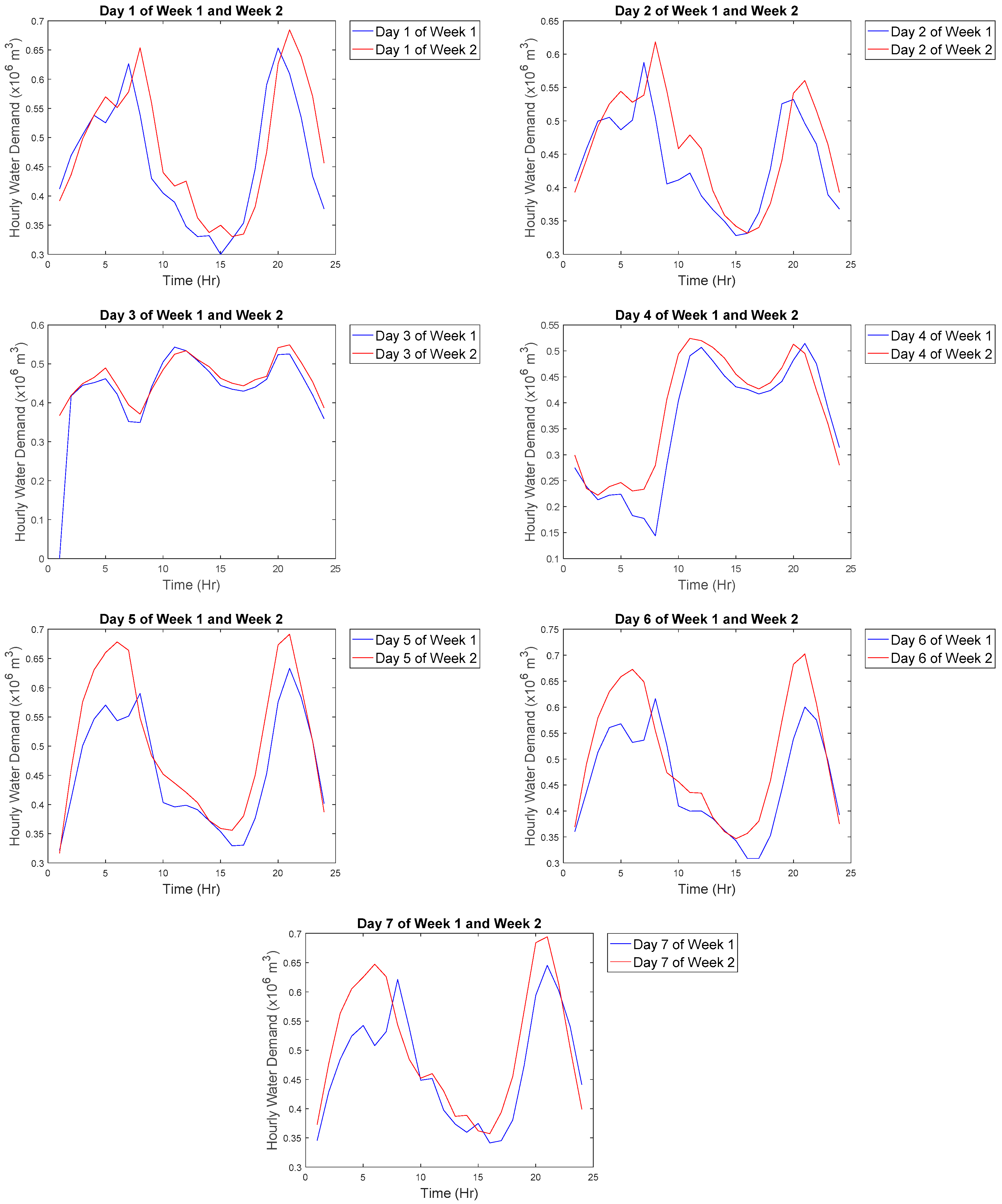
To get an idea of the water demand on each day, the first two weeks of the data with the assumption that data collection starts at 01:00 were analyzed and the graphs can be seen in Figure 1. The majority of the days displayed a general trend of increasing water demand in the early morning with peaks at approximately 07:00–08:00 and a decreasing trend after that. Water demand then peaks again at approximately 20:00 and 21:00 before decreasing again. The days that do not follow the trends are Day 3 and Day 4 in each week. Based on the results, Day 3 and Day 4 are assumed as rest days or weekend and the rest of the days are workdays or weekdays. Water demand peaks in the morning due to working adults are preparing to go for work, water demand drops in the afternoon when they are not at home. Once the working adults come home, the demand rises again. As they are not working on the weekend, it can be seen from the graph (Day 3 and Day 4) that water demand does not follow the weekday trend. The adults may go to bed in the wee hour. Hence, the water demand peaks slightly later in the early morning. The water demand does not have a drastic drop in the afternoon as compared to the weekday trend as the working adults can be at home over the weekend. Such a phenomenon is also discussed in [11] and [23].

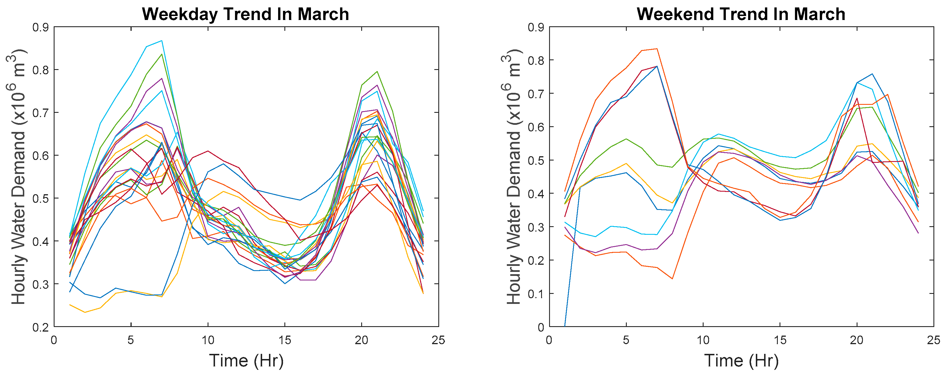
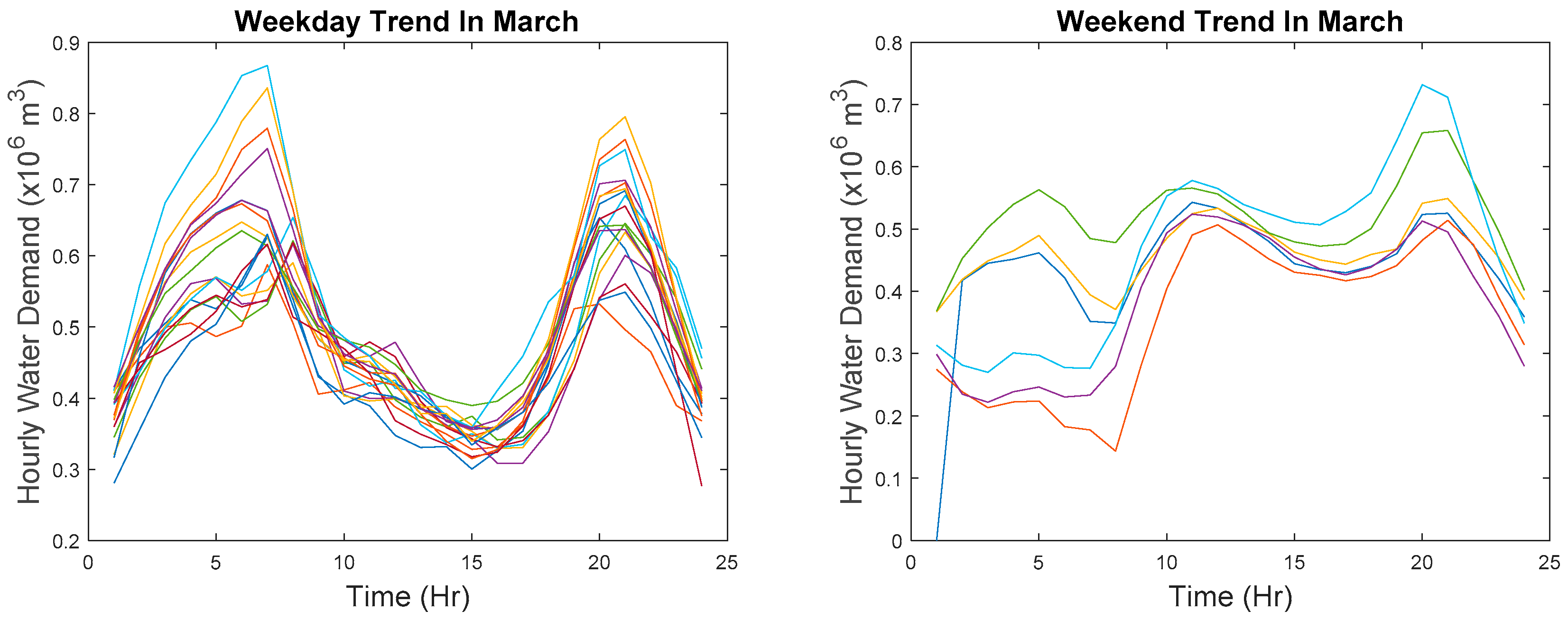
Looking at the 2012 calendar, 1 March 2012 is on a Thursday whereas 3 and 4 March 2012 are on the weekend. That coincides with the explanation given above. Therefore, it can be deduced that data collection starts from 1 March 2012 and ends on 29 December 2012 in order to match the number of data points available. Based on such deductions, the weekday and weekend trends of March are plotted. The majority of the weekday trends generally follows the explanation given above. A minority that does not follow such a trend follows the weekend trend instead. It could be due to the day being a public holiday resulted in the weekend trend. Similarly, the majority of the weekend trend follows our explanation given above although there are several weekends following the weekday trend instead. It could be due to a large group of families going on an excursion on the weekend; that is why water demand is higher in the morning as they are preparing to go out. The water demand then drops after they are out and increases when they reach home. Alternatively, it can be due to an unexpected event.

In the dataset, all data collected are unlabeled, and there is a missing data point in March and a total of 165 missing data points from April onwards. The missing points from April onwards are imputed with random values to represent the anomalous points present in the data. This is done according to the following formula.

$$Random Value=\max \left(data\right)\times 1.1\times rand\left(1\right)$$

(1)

In addition to the imputed anomalous points, the data are assumed to contain other anomalous points or trends which are not labeled. Therefore, the motivation of the proposed approach is to detect any abnormal trend of points present in the data that does not conform to the usual pattern or trend using a minimal set of unlabeled data. Accuracy of proposed algorithm will be tabulated based on the detected imputed anomalous points.

Note that the data collected in March are used as reference data for subsequent anomaly detection in this paper which is why the missing data point in March was not imputed with a random value to prevent the inclusion of the noise and is excluded instead. By comparing the amount of data required, proposed methodology will only utilize a month of data while Candelieri [11] requires at least a year of data for the identification of seasonality and Wu et al. [13] requires at least six months of data.

3. Proposed Approach

As discussed by Zhang et al. [24], there are three different main objectives with different approaches in clustering time series.

• Similarity in time—to cluster series that varies in a similar way at each time step;
• Similarity in change—to cluster series by the similarity in how they vary from each time step;
• Similarity in shape of the trend—to cluster series with common shapes together.

However, these approaches may not be suitable for real-time detection and require at least several points to form a series before any matching of series can be performed. The proposed approach adopts the same principles with several adjustments to accommodate real-time anomaly detection.

• Similarity in time—to cluster points that are relatively similar at each time step;
• Similarity in change—to cluster points at each time step by the similarity in how they vary from each time step;
• Similarity in shape of the trend—to compare the incoming points with a reference shape for online anomalous trend detection.

It is important to state that the proposed approach is meant to carry out all the three objectives at the same time. The rationale behind doing it this way is given in Section 3.4. Section 3.1 describes how we prepare the data, followed by the description of the algorithm used to achieve objective 1 and 2. Section 3.2 then describes the algorithm used to achieve objective 3.

3.1. Data Preparation

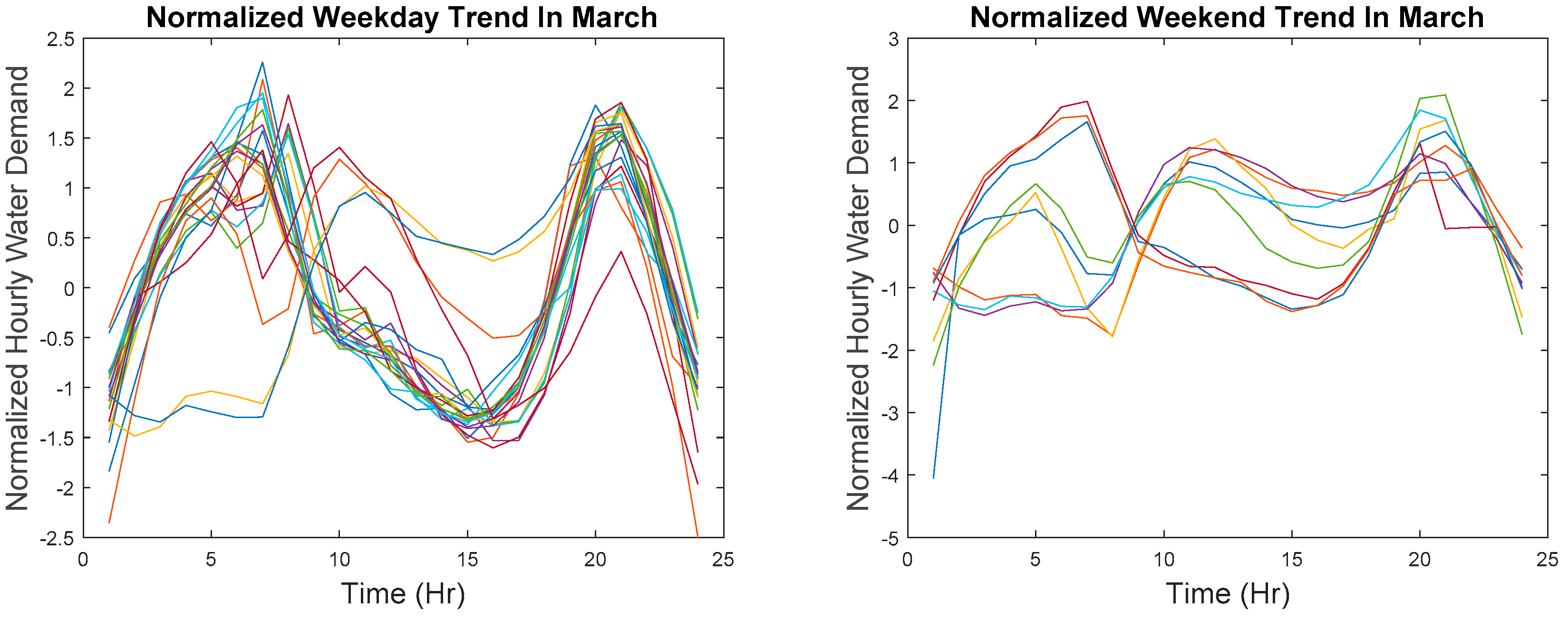
In order to cluster points that are relatively similar at each time step, the reference data must first partition into weekday and weekend data because demand patterns for weekday and weekend are entirely different. The difference in shape can be seen in Figure 2 which is plotted in actual values and in Figure 3 where data are z-score normalized. The partitioned data are then transformed by aligning the hour on different days. Recall that data collected in March are used as reference data and also recall that there is a missing data point in March but to avoid any mathematical confusion, the subsequent explanation is based on the assumption that there are no missing data points. However, in the actual implementation of the algorithm, the missing data point is excluded.

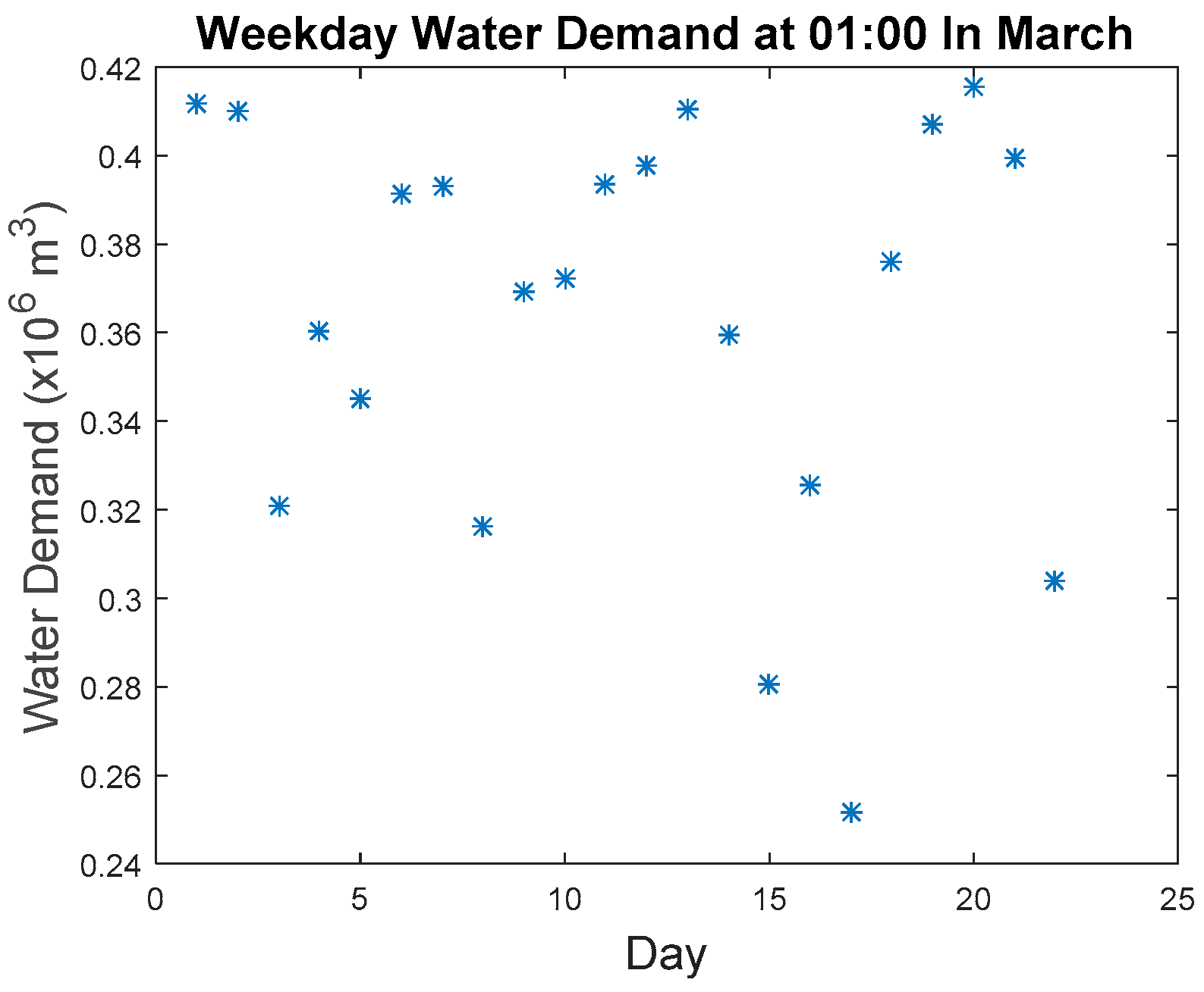
The total number of data points in March is 744 (31 days with 24 points per day) and in March 2012, there were a total of 22 weekdays and nine weekends. Therefore, the weekday vector of size 528 × 1 is reshaped into a 24 × 22 matrix and weekend vector of size 216 × 1 is reshaped into 24 × 9 matrix where the row of the matrix represents the hour while the column represents the different days. As suggested in the literature [13,23,25], this transformation is performed to reduce the level of fluctuation in a hourly series. By referring to Figure 4, the level of fluctuation is indeed lower as compared to the hourly water demand pattern.

To achieve the second objective, the first derivative using the following equation except the first data point is computed. Since the first point, $W_1$, does not have any reference point, $W_{t-1}$, $\frac{dW}{dt}$ for the first data, the point is assumed zero.

$$\frac{dW}{dt}=\frac{W_t-W_{t-1}}{\Delta t},$$

(2)

where $W_t$ is the hourly water demand at time t, $\Delta t$ refers to the change in time, and $\frac{dW}{dt}$ refers to the rate of change of hourly water demand with respect to time. The computed first derivative for the month of March is a vector of size 744 × 1. Similarly, the calculated first derivative is partitioned into weekday and weekend data and transformed by aligning the hour of different days that gives a weekday first derivative matrix of size 24 × 22 and a weekend first derivative matrix of size 24 × 9.

3.2. Dirichlet Process Mixture Model

A representative example of BNP model used in the application of clustering is the DPMM [18]. In this section, the general idea of a DPMM and how it is applied in this case study is provided. For a better understanding of DPMM, readers are encouraged to read [16,18,26,27]. DPMM is an infinite mixture model [26] where the number of the components in a finite mixture model approaches infinity. A finite mixture model can be represented as [16,27]:

$$\pi |a~Dir\left(\frac{a}{K},\dots ,\frac{a}{K}\right)$$

(3)

$${\theta }_k|G_0~G_0$$

(4)

$$z_n|\pi ~\pi$$

(5)

$$y_n|z_n,{\theta }_k~F\left({\theta }_{z_n}\right)$$

(6)

The equations can be explained as follows. Given that $Y$ is a set of data with $n$ observations, $Y=\left\{y_1,\dots ,y_n\right\}$, $F$ is the generative distribution of $Y$ and is parameterized by $K$ number of $\theta$, where $K$ is the number of components/clusters. Each $\theta$ contains a set of parameters which is assumed to follow a base distribution $G_0$. The class assignment $z$ which ranges from 1 to $K$ is drawn from a multinomial distribution given $\pi$ which contains the mixture probabilities of the components. On the other hand, $\pi$ follows a symmetrical Dirichlet distribution n, where $a$ is the concentration parameter. The Dirichlet distribution is a distribution over (K − 1) dimensional simplex; which can be said as a distribution over the relative values of K components, where the sum is 1.

Therefore, as $K$ approaches infinity, it becomes a DPMM that can be represented as [16,27]:

$$G~DP\left(a,G_0\right)$$

(7)

$${\varnothing }_i|G~G$$

(8)

$$y_i|{\varnothing }_i~F\left({\varnothing }_i\right)$$

(9)

The equations imply drawing of random probability measure $G$ from a Dirichlet Process (DP) given $a$ and $G_0$. $y_i$ is drawn from a mixture of distribution of form $F\left({\varnothing }_i\right)$ where mixing distribution over ${\varnothing }_i$ is $G$ [27].

The prior over the clusters defined in the DPMM used is the Chinese Restaurant Process (CRP) [16]. The metaphor was originally devised by Dubins and Pitman as a way of constructing consistent random permutations and partition [28]. The CRP can be described as follows. Imagine a restaurant with an infinite number of tables and there is no limit as to how many customers can sit at one table. The ith customer who walks into the restaurant has the probability of sitting at table K proportional to the number of customers already seated at table K. However, the ith customer still has a probability of choosing to sit at an unoccupied table. This phenomenon is depicted in Figure 5.

Therefore, the prior of the new data point i can be formally defined as [16]

$$P\left(PointitojoinclusterK\right)=\frac{N}{a+i-1},$$

(10)

$$P\left(Pointitostartanewcluster\right)=\frac{a}{a+i-1},$$

(11)

where a is the concentration parameter and N is the number of observations in cluster K. Such prior implies a rich get richer property since new data point has a higher probability of joining the majority cluster. As anomalies are rare [15], normal data points will form the majority in the same cluster. Therefore, if a new data point gets labeled as a member of a new cluster even with the “bias” prior, it can be considered as an anomaly.

The idea of the proposed approach is to apply DPMM on our transformed hourly demand and calculated first derivative data, which will produce a set of statistics for each hour for every cluster identified in that particular hour which can be seen in Figure 6. These sets of statistics are cached and updated whenever a new data point arrives.

3.3. Incremental Similarity Tracking Using Time Warp Edit Distance

To achieve the third objective of the proposed approach, the proposed idea is to compare the incoming points with a reference shape, which requires a form of similarity metric. In this paper, the Time Wrap Edit Distance (TWED) is used. The formal definition for this metric is given as follows [29].

$${\delta }_{\lambda ,v}\left(A_1^p,B_1^q\right)=min\{\begin{array}{c}{\delta }_{\lambda ,v}\left(A_1^{p-1},B_1^q\right)+г\left(a_p^{\prime }\to \Lambda \right)\hspace{1em}delet{e}_A\\ {\delta }_{\lambda ,v}\left(A_1^{p-1},B_1^{q-1}\right)+г\left(a_p^{\prime }\to b_q^{\prime }\right)\hspace{1em}match\\ {\delta }_{\lambda ,v}\left(A_1^p,B_1^{q-1}\right)+г\left(\Lambda \to b_q^{\prime }\right)\hspace{1em}delet{e}_B\end{array},$$

(12)

with

$$г\left(a_p^{\prime }\to \Lambda \right)=d\left(a_p^{\prime },a_{p-1}^{\prime }\right)+\lambda$$

(13)

$$г\left(a_p^{\prime }\to b_q^{\prime }\right)=d\left(a_p^{\prime },b_q^{\prime }\right)+d\left(a_{p-1}^{\prime },b_{q-1}^{\prime }\right)$$

(14)

$$г\left(\Lambda \to b_q^{\prime }\right)=d\left(b_p^{\prime },b_{p-1}^{\prime }\right)+\lambda$$

(15)

The recursive algorithm is initialized as follow:

$${\delta }_{\lambda ,v}\left(A_1^0,B_1^0\right)=0,$$

(16)

$${\delta }_{\lambda ,v}\left(A_1^0,B_1^j\right)=\infty forj\ge 1,$$

(17)

$${\delta }_{\lambda ,v}\left(A_1^i,B_1^0\right)=\infty fori\ge 1,$$

(18)

where ${\delta }_{\lambda ,v}$ is a distance on the set of finite discrete time series. $A_1^p$ and $B_1^q$ are time series with discrete-time index varying between 1 to p or q. $a_p^{\prime }$ and $b_q^{\prime }$ represent the $p\mathrm{th}$ and $q\mathrm{th}$ sample of time series A and B, respectively. $г$ is an arbitrary cost function which assigns a non-negative real number and is given as 0.01. $\lambda$ which has a value of zero or bigger than zero is a constant penalty. Finally, $d(·)$ is a distance in between the Minkowski’s Distance, which is characterized by a kind of “infinite stiffness”, and Dynamic Time Warping (DTW), which is characterized by a “null stiffness”.

As explained by Marteau [29], Euclidean distance is a nonelastic metric that does not support time-shifting whereas elastic similarity measure such as DTW is not a metric since they do not satisfy the triangle inequality. On the other hand, TWED is an elastic metric that takes time stamp into account. Moreover, empirical evaluation has shown that TWED performs better than Euclidean distance, DTW, and edit distance with Penalty [29]. Hence, it makes an appropriate choice in this paper.

To fulfill the criteria of online anomalous shape tracking, instead of waiting for the batch data to measure the similarity between the new series and the reference series, the similarity will be computed at every hour with the pseudocode as shown in Algorithm 1.

Algorithm: Incremental Similarity Tracking Using TWED.

The steps in the proposed Incremental Similarity Tracking using TWED follow the following sequence.

• Among the weekday and weekend series deemed to follow a normal trend, determine the median, 20th, and 80th percentile for each hour;
• Based on the 20th and 80th percentile, compute the interquartile range which is to determine the difference between the two percentiles;
• Calculate the lower and upper bound for each hour as follows:

  $$\mathrm{a}.\hspace{1em}Lower Bound= 20th Percentile-1.5\times Interquartile Range$$

  (19)

  $$\mathrm{b}.\hspace{1em}Upper Bound= 80th Percentile+1.5\times Interquartile Range$$

  (20)
• Form a reference series using all median found at each hour;
• Form a lower bound series using all lower bound calculated at each hour;
• Form an upper bound series using all upper bound calculated at each hour;
• Compute the similarity between the weekday reference series and weekday lower bound series at the different time of the day:
  • Do for n ← 1:24;
  • If n = 1;
  • Calculate the Euclidean distance between the first point of reference series and first point of lower bound series;
  • Else if n > 1;
  • Z-score normalizes the first n points of reference series and lowers bound series, respectively. Subsequently, compute the similarity between these two partial series using the TWED;
  • End if;
  • End for;
  • At the end of for loop, there are 24 points, each representing the level of similarity at a different time of the day. Concatenate the points to form a weekday similarity matrix, M1.
• Using a similar procedure, calculate the similarity between the reference series and the upper bound series to obtain the second similarity matrix, M2;
• Find the mean of M1 and M2 at a different time of the day to obtain the maximum weekday allowable dissimilarity vector of size 24 × 1. This is to take the dissimilarity between the reference series with both the lower and upper bound series into consideration;
• Repeat Step 7 to 9 to find the maximum weekend allowable dissimilarity matrix;
• For every new day starting with data collected at 01:00, perform Steps 7a to 7g to calculate the similarity between the new day and the reference series. If the new day is a weekday, then the reference series used should be the weekday reference series;
• Find all points in the new day that gives similarity value that is higher than the value in the maximum allowable dissimilarity matrix. Such points are considered as anomalies.

To explain the procedure in detail, first extract series are not considered an anomaly series. For example, weekday should only have weekday trends whereas weekend should only have weekend trends as shown in Figure 7. The first weekend of March has a missing point where it is replaced with a zero.

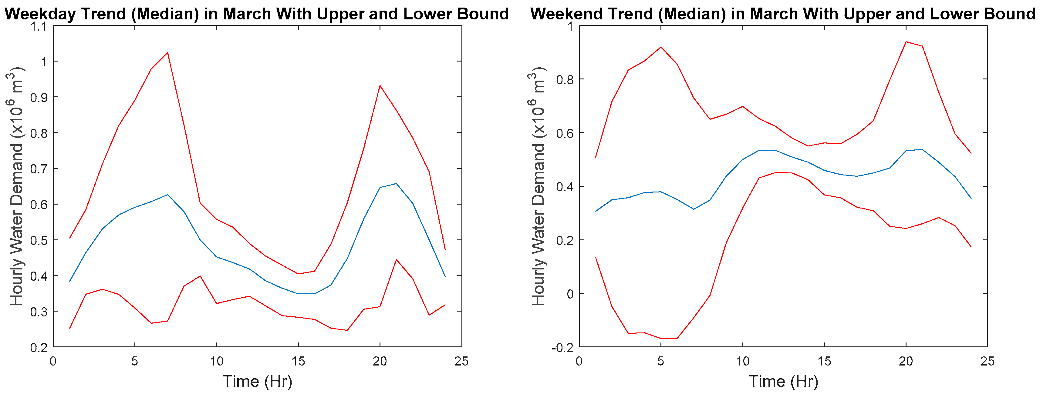
Based on the extracted profiles for weekday and weekend, the median, 20th, and 80th percentile of water demand at each hour are computed. Using the 20th and 80th percentile, the interquartile range is then calculated. Finally, the lower bound and the upper bound at each hour are determined using the percentiles and the interquartile range at each hour. The medians, lower bounds, and upper bounds for weekday and weekend are joined together to form a series, respectively, as shown in Figure 8.

The degree of similarity is computed between the median series and the lower and upper bound series at each hour with the inclusion of previous points. Since the first point collected at the first hour has no previous point, Euclidean distance is determined between the first point of the median series and the first point of the lower and upper bound series. From the second hour onwards, all previous points of the day are combined to form a series. Before the comparison, each time series is normalized to a mean of zero and a standard deviation of one so as to avoid comparing time series with different offsets and amplitude [30]. Finally, the similarity between the median series, the lower and upper bounds series is computed using TWED, where

Table 1. Similarity for weekday median series against upper and lower bound series.

Time	Data Points Collected for Comparison	Similarity with Lower Bound	Similarity with Upper Bound	Mean/Max Allowable Dissimilarity
01:00	0:100	0.132	0.121	0.127
02:00	01:00–02:00	0.000	0.000	0.000
03:00	01:00–03:00	1.278	0.768	1.023
04:00	01:00–04:00	2.705	1.253	1.979
05:00	01:00–05:00	5.245	1.535	3.390
06:00	01:00–06:00	8.382	2.152	5.267
07:00	01:00–07:00	11.434	2.732	7.083
08:00	01:00–08:00	13.648	3.352	8.500
09:00	01:00–09:00	14.778	3.869	9.323
10:00	01:00–10:00	15.763	4.246	10.005
11:00	01:00–11:00	16.210	4.301	10.255
12:00	01:00–12:00	17.439	4.232	10.835
13:00	01:00–13:00	19.514	4.455	11.984
14:00	01:00–14:00	19.848	4.922	12.385
15:00	01:00–15:00	19.777	5.293	12.535
16:00	01:00–16:00	19.726	5.620	12.673
17:00	01:00–17:00	19.977	6.107	13.042
18:00	01:00–18:00	21.080	6.677	13.878
19:00	01:00–19:00	22.343	7.094	14.719
20:00	01:00–20:00	23.690	7.213	15.452
21:00	01:00–21:00	21.897	7.609	14.753
22:00	01:00–22:00	22.762	8.547	15.655
23:00	01:00–23:00	24.089	9.263	16.676
24:00	01:00–24:00	25.994	9.402	17.698

and

Table 2. Similarity table for weekend median series against upper and lower bound series.

Time	Data Points Used for Comparison	Similarity with Lower Bound	Similarity with Upper Bound	Mean/Max Allowable Dissimilarity
01:00	01:00	0.171	0.201	0.186
02:00	01:00–02:00	4.243	0.000	2.121
03:00	01:00–03:00	7.299	0.788	4.043
04:00	01:00–04:00	9.417	1.066	5.241
05:00	01:00–05:00	12.303	1.314	6.809
06:00	01:00–06:00	15.135	2.473	8.804
07:00	01:00–07:00	17.011	4.773	10.892
08:00	01:00–08:00	18.186	6.513	12.349
09:00	01:00–09:00	15.332	10.081	12.706
10:00	01:00–10:00	11.948	13.785	12.867
11:00	01:00–11:00	10.256	16.312	13.284
12:00	01:00–12:00	9.415	18.780	14.098
13:00	01:00–13:00	9.494	20.881	15.187
14:00	01:00–14:00	10.064	22.350	16.207
15:00	01:00–15:00	11.088	23.184	17.136
16:00	01:00–16:00	12.326	23.616	17.971
17:00	01:00–17:00	13.581	24.527	19.054
18:00	01:00–18:00	14.583	26.270	20.426
19:00	01:00–19:00	15.369	27.239	21.304
20:00	01:00–20:00	16.850	27.191	22.021
21:00	01:00–21:00	17.409	27.353	22.381
22:00	01:00–22:00	18.879	28.326	23.603
23:00	01:00–23:00	19.750	29.570	24.660
24:00	01:00–24:00	21.236	30.313	25.775

present the results from the proposed algorithm. As observed in Table 1 and Table 2, the lower the value, the higher is the similarity between the two series. As seen in Table 1 and Table 2, if the similarity is calculated using only two data points where the curves have the same trends then the calculated TWED is zero. The maximum allowable dissimilarity column refers to the maximum allowable distance/dissimilarity between the two series in each hour. This value is calculated using the average of the similarity with lower bound and the similarity with the upper bound. Note that the lower the value of the lower bound percentile (i.e., 15th percentile) and the higher the value of the upper bound percentile (i.e., 85th percentile), it results in a higher maximum allowable distance/dissimilarity.

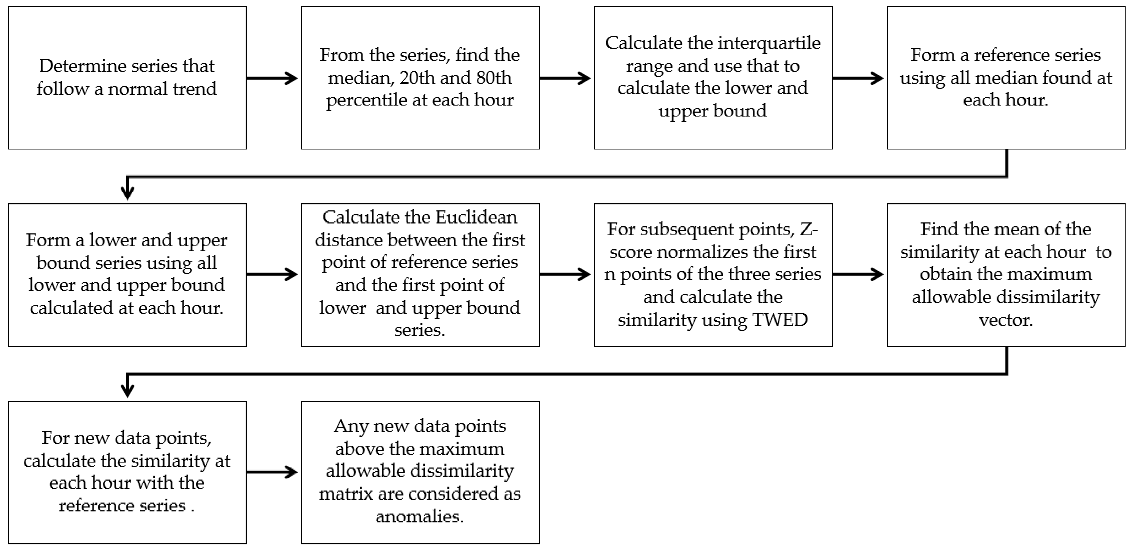
In order to calculate the similarity of future series with the median series, the point collected at 01:00 will always be the first point of a new series and the point collected at 24:00 is the last point of the new series. The procedure to calculate the similarity between the two series has been described in the previous paragraph. If the calculated similarity value exceeds the value in the maximum allowable dissimilarity column at each hour, then an anomaly has occurred in that particular hour. A flowchart of the entire procedure is also summarized in Figure 9.

3.4. Rationale

As discussed earlier, the proposed approach is meant to carry out all the three objectives, namely to track (1) similarity in time, (2) similarity in the rate of change, and (3) similarity in the shape of the trend. By tracking only the similarity in time or change at a specific hour, it can cause a false negative or a false positive.

The limitation of tracking the similarity in time is that we cannot detect any anomalous trend present in the hourly series. For example, at 08:00, there exists an anomalous point. However, at 09:00, the series becomes normal then at 10:00; there is another anomalous point. Hence, tracking the similarity solely in time cannot detect data collected at 09:00 as an anomalous point. Whereas, if an anomalous water demand appears with an anomalous rate of change, then we can easily track this type of anomaly. However, if the subsequent water demand collected has an anomalous value with a normal rate of change, it is not possible to detect such anomalous point as the rate of change is considered as normal.

On the other hand, shape tracking is useful in finding an anomalous trend. However, there may be false negatives due to the maximum allowable dissimilarity. The maximum allowable maximum dissimilarity allows some tolerance to the shape when compared with the reference trend. Therefore, if the similarity between the reference series and a series formed by the incoming anomalous point with the previous points do not exceed the maximum allowable dissimilarity, then such anomaly will be disregarded.

In order to consider all three objectives simultaneously, a scoring system is proposed. If any point is found to be anomalous either in value, rate of change, or shape, a score will be given. Any point with at least one in the score will be detected as an anomaly because they satisfied the condition of the anomalous value, the anomalous rate of change, or/and the anomalous shape.

4. Results and Discussion

In this section, results of the proposed approach are discussed. The workstation used in this study is a 64 bit operating system and comes with an Intel i7-5500U [email protected] processor with a 16GB ram installed. The proposed approach is carried out in a MATLAB environment (MATLAB 2018b) and is programmed to handle streaming data point. Thus, computational time for each new data point can be completed in seconds.

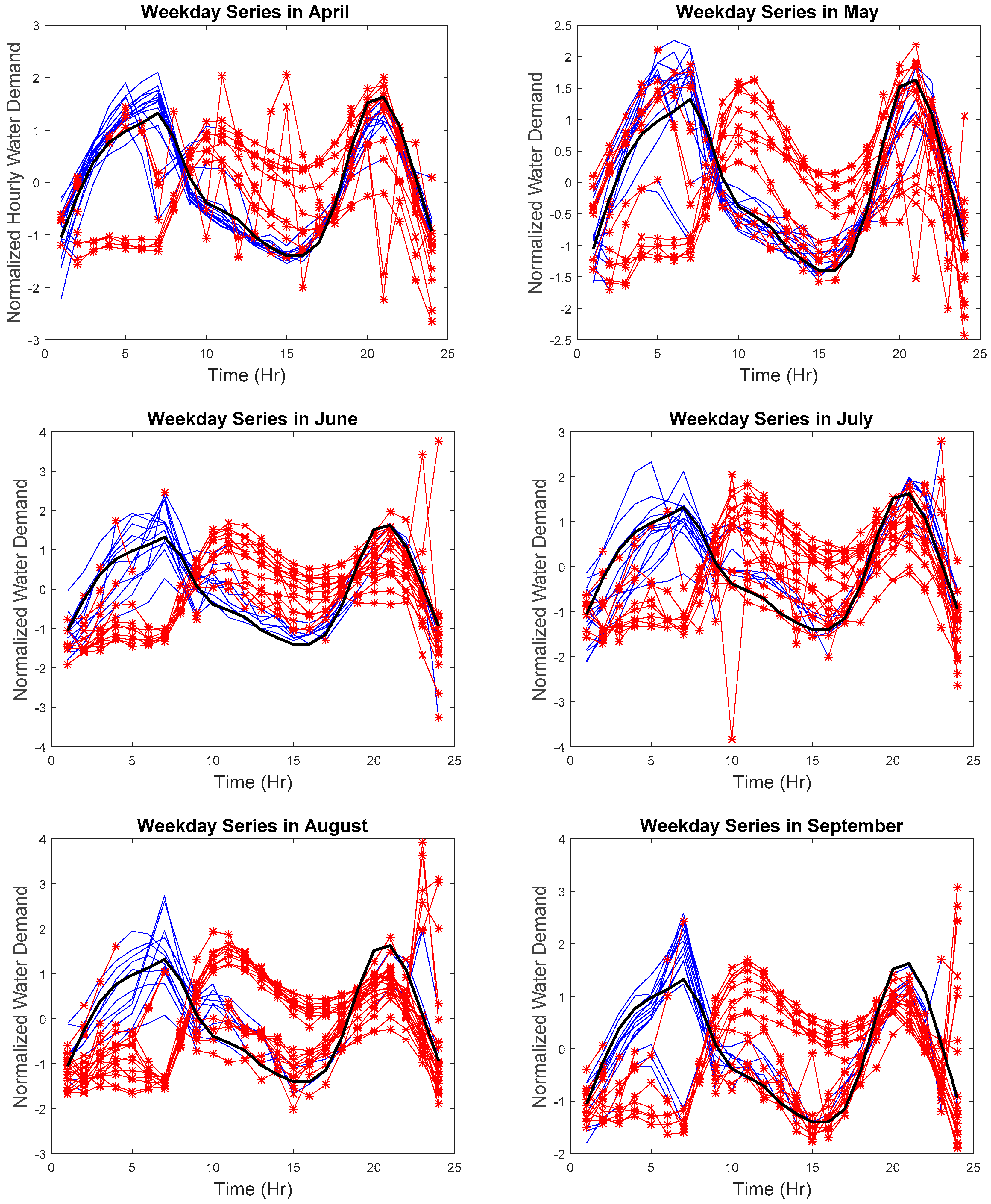
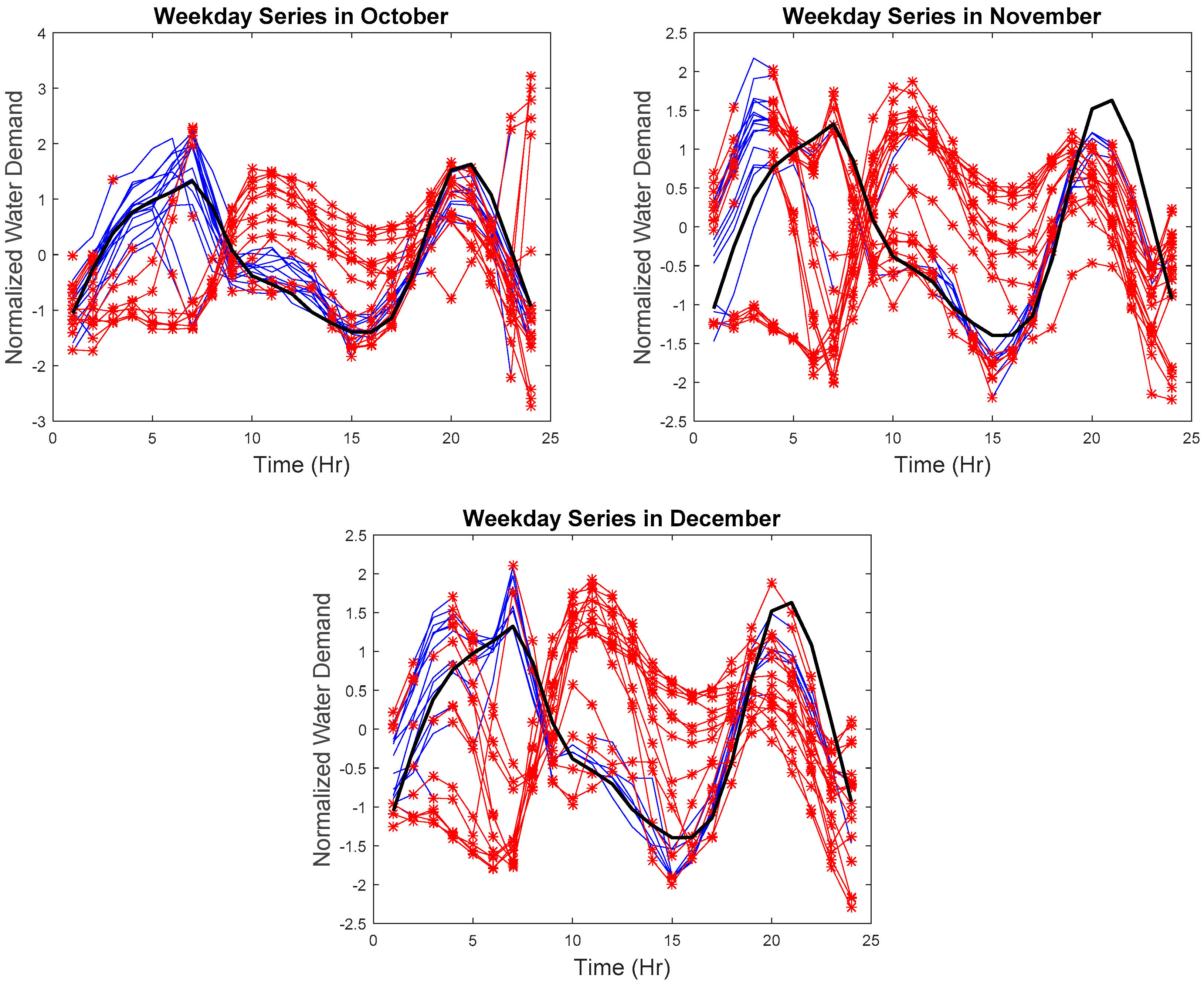
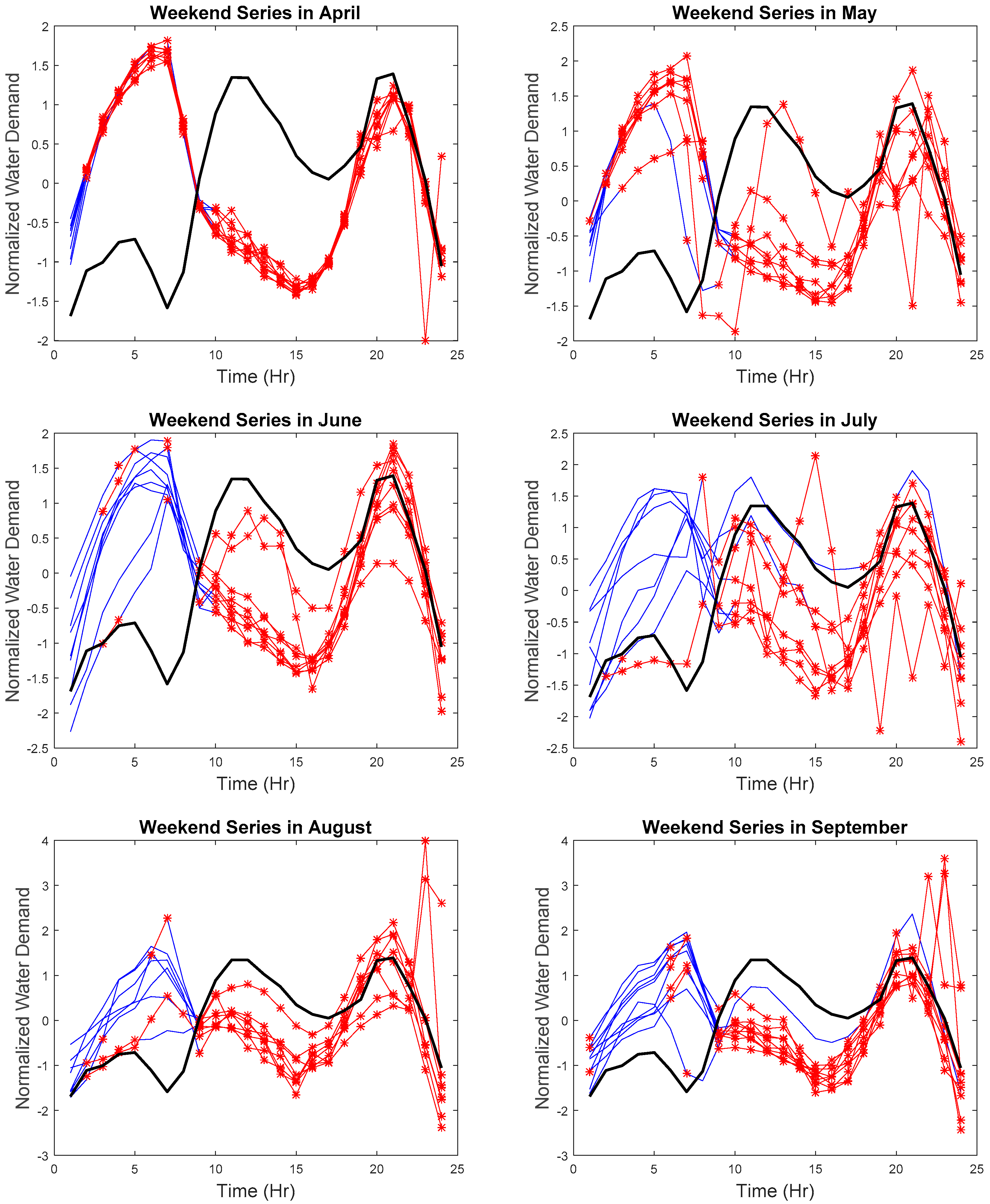
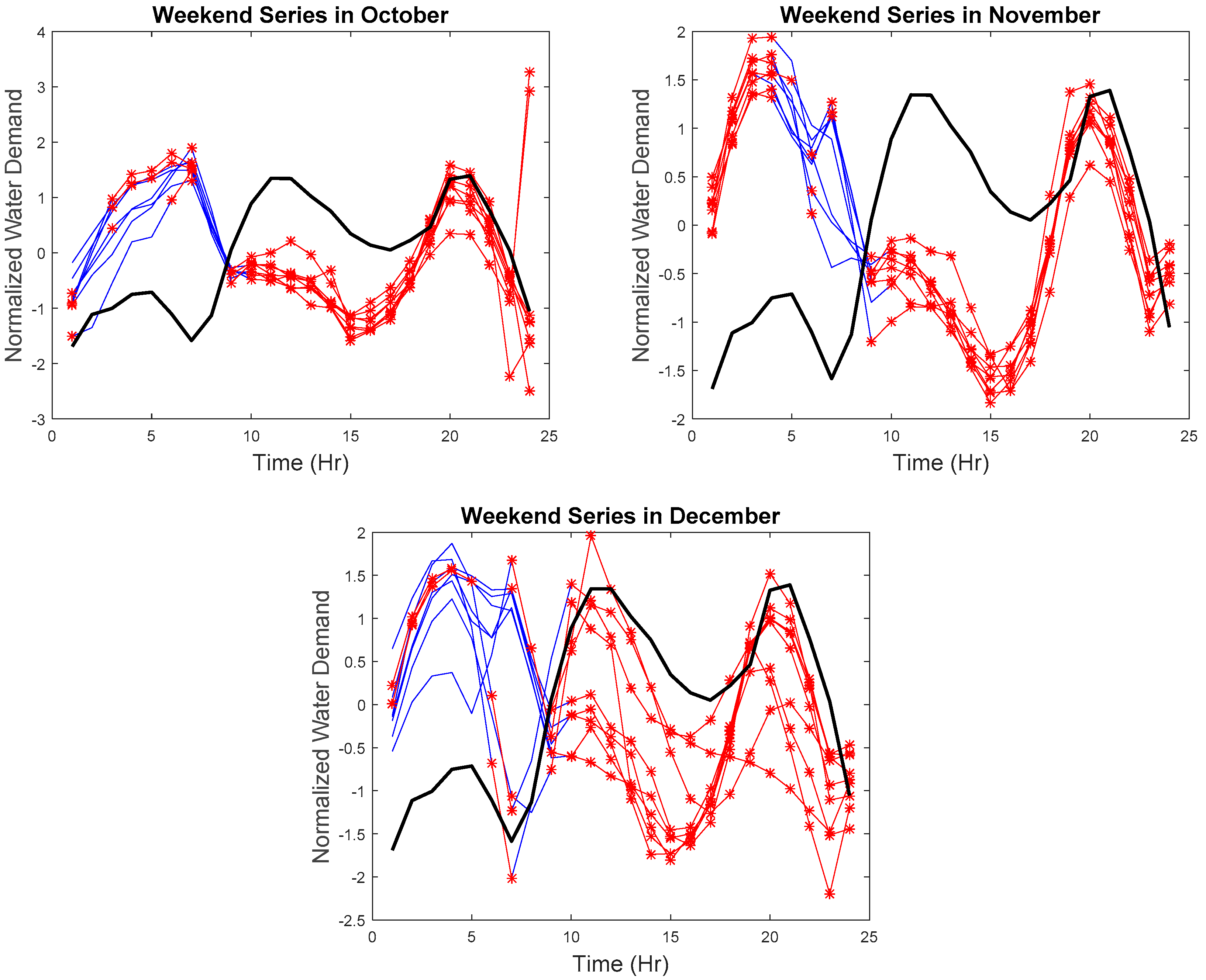
Due to the space limitation, the hourly series with the detected anomalies will not be displayed. Therefore, results are presented in z-score normalized weekday and weekend monthly series, as seen in Figure 10, Figure 11, Figure 12 and Figure 13, respectively. The blue lines are the collected data for each day, the red lines are the detected anomalies, and the black line is the reference curve.

As seen in Figure 10 and Figure 11, the hourly weekday series not following the weekday trend was identified. Abnormal weekday trend with several spikes can be seen in April. Any sharp drop or increase in the hourly water demand was also identified in May, June, July, and November. The hourly weekend series with abnormal trends, abnormal increase, or decrease were also identified. Such results suggest the effectiveness of our proposed approach to tracking the (1) similarity in time, (2) the similarity in the rate of change, and (3) the similarity in shape where any discrepancies in the hourly series can be found in real-time.

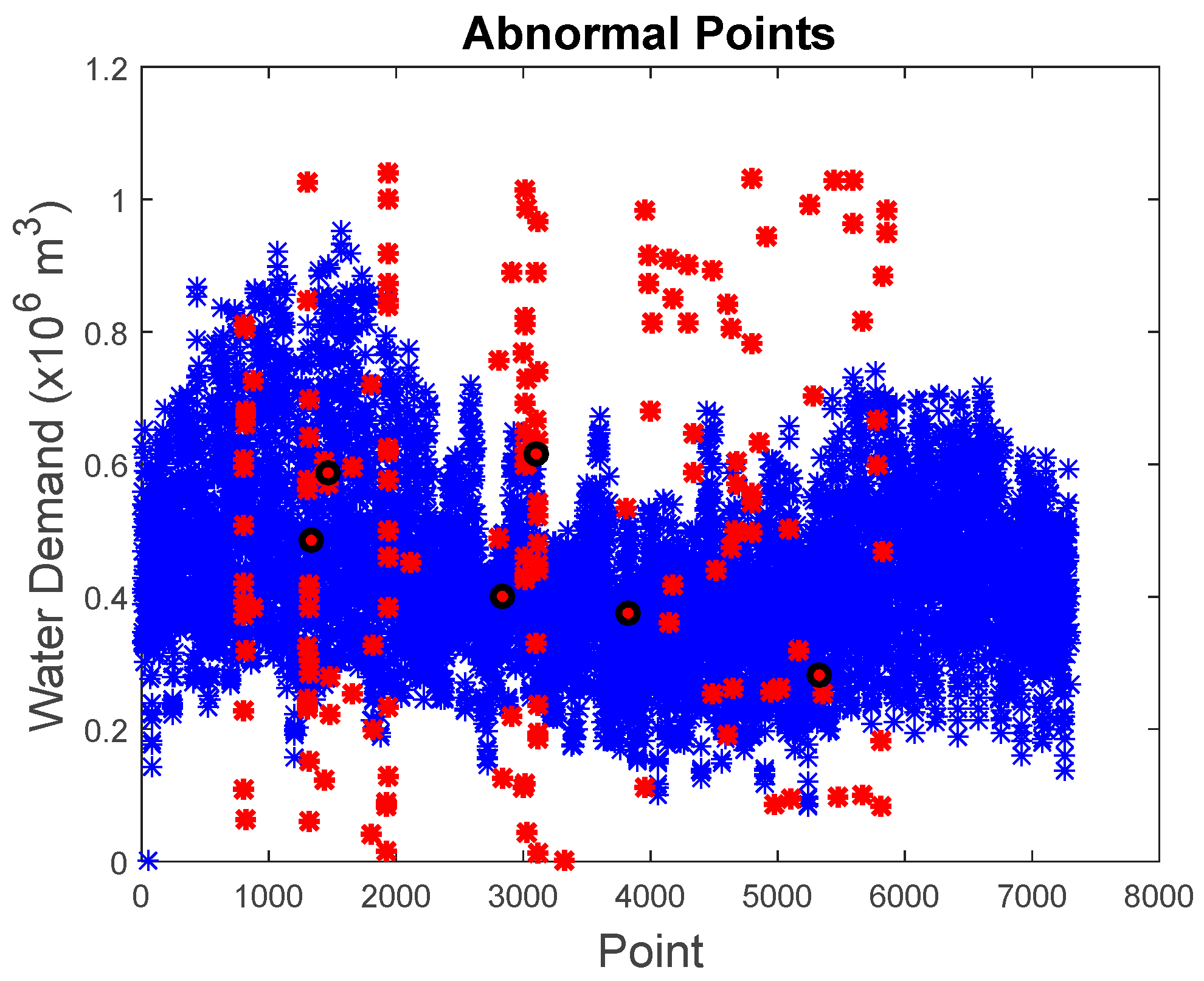
As mentioned earlier, the accuracy of the proposed algorithm will be tabulated based on the detected imputed anomalous points. Figure 14 shows the water demand values of all the imputed anomalous point as compared to the original data points. The detection accuracy based on the detected imputed anomalous points is at 96% where there are a total of six missed detections among 165 known anomalies. The parameters for the six missed detected anomalies are shown in

Table 3. Parameters of missed detected anomalies.

No	Month	Day of Week	Date	Time	Water Demand (Mega Cubic Meter)	First Derivative (Mega Cubic Meter)
1	4	3	25	09:00	0.486	−0.1574
2	4	1	30	23:00	0.5882	−0.1246
3	6	2	26	23:00	0.4013	−0.0725
5	8	1	6	24:00	0.3740	−0.1602
6	10	1	8	24:00	0.2828	−0.0927
4	7	7	8	07:00	162.261	−0.436

. By examining these points, five of the six points were showing patterns similar to a normal value that leads to missed detection. The other missed detected anomaly was due to the sensitivity of our proposed approaches. It is not sensitive enough to detect small developing anomalous trends present within the maximum allowable similarity.

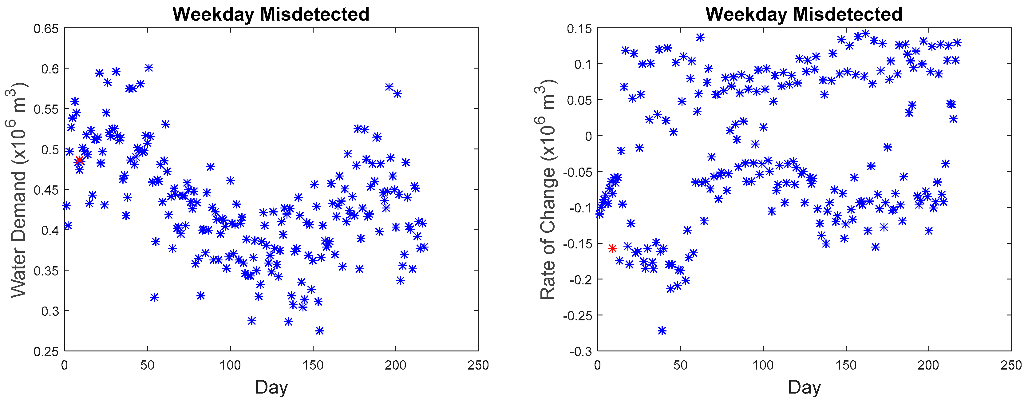
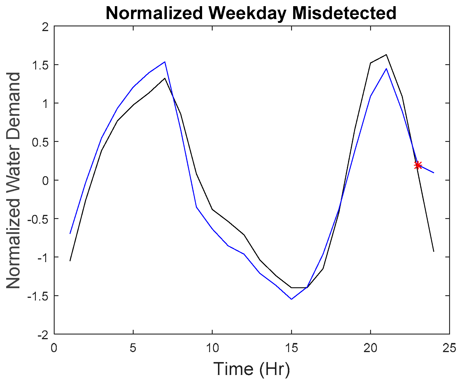
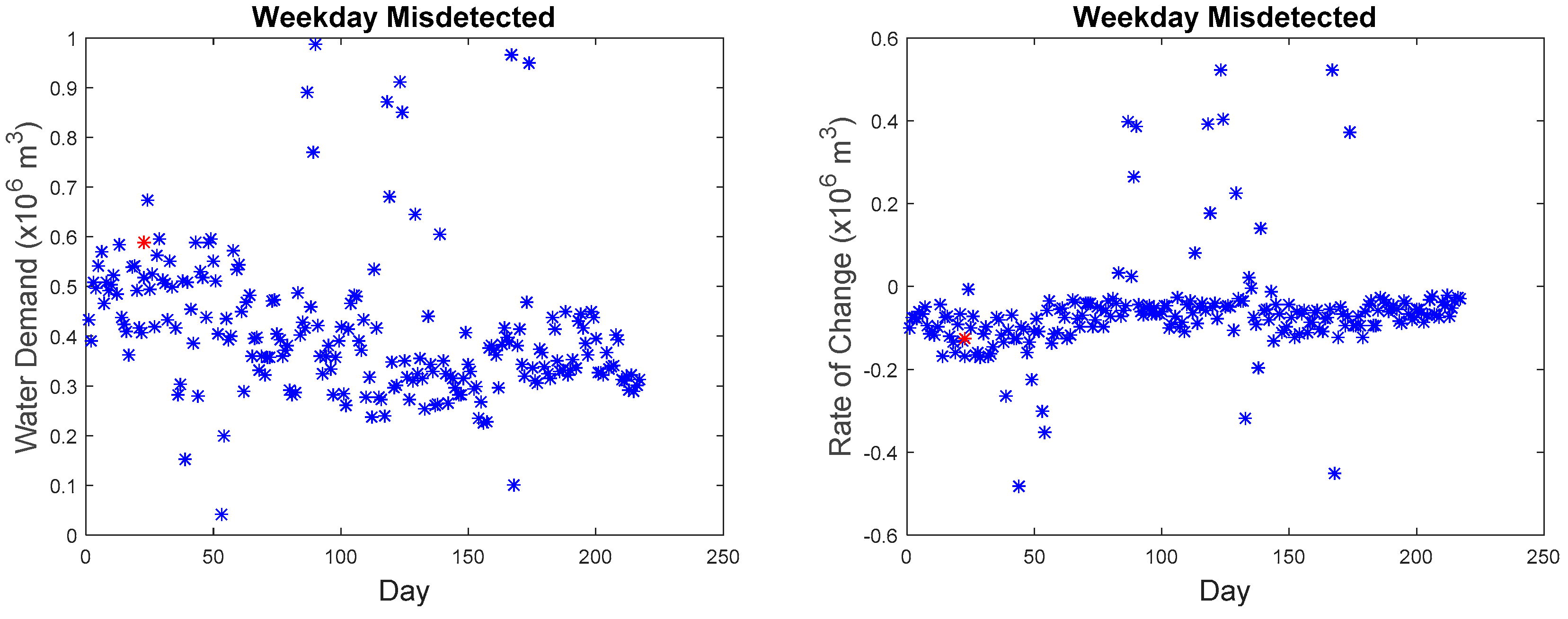
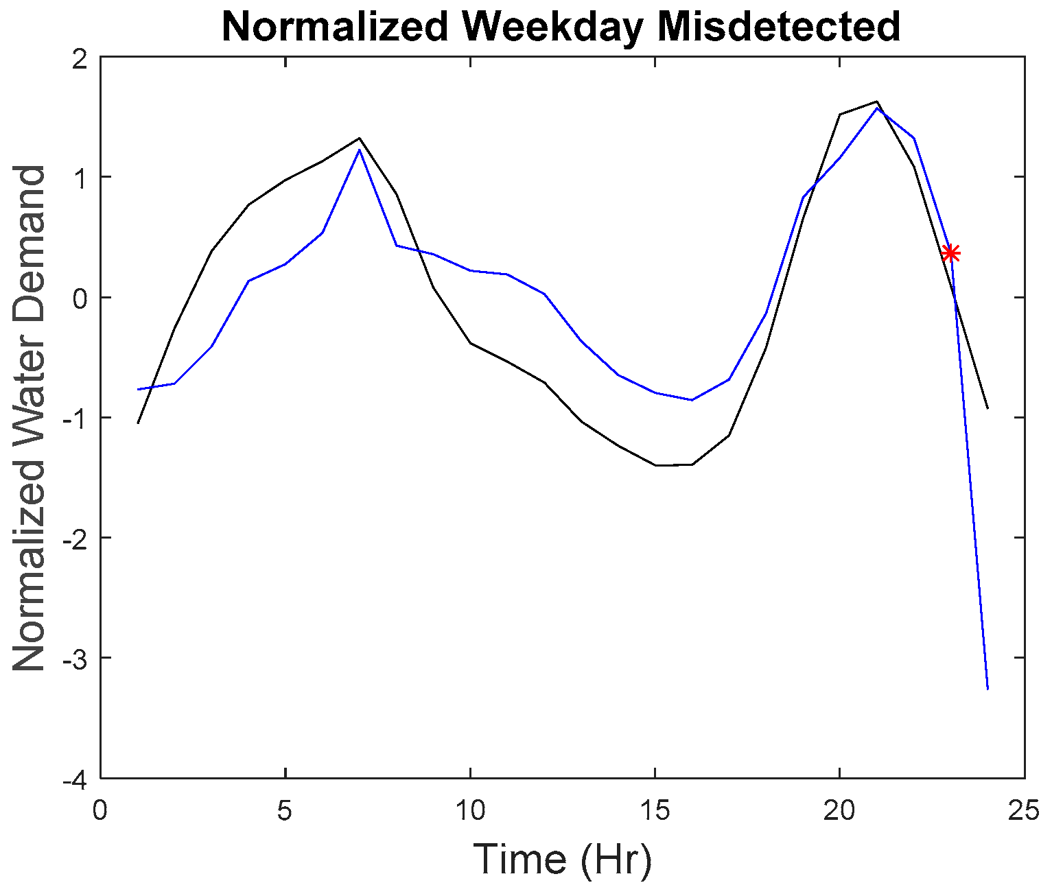
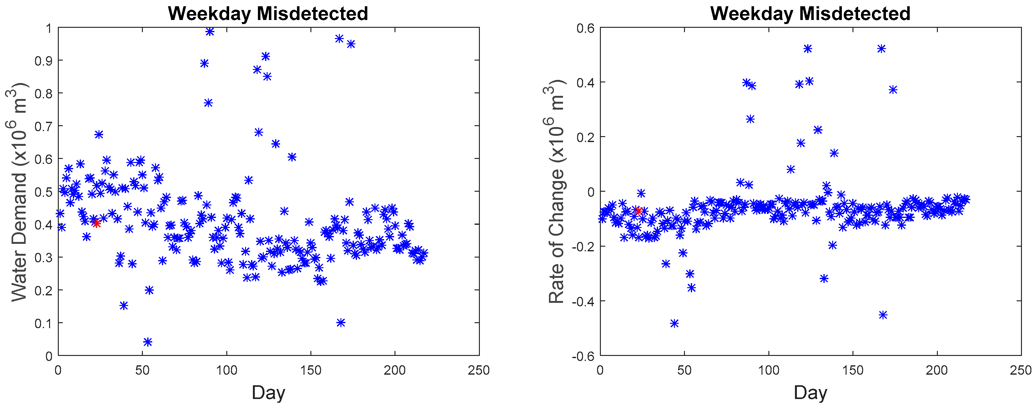
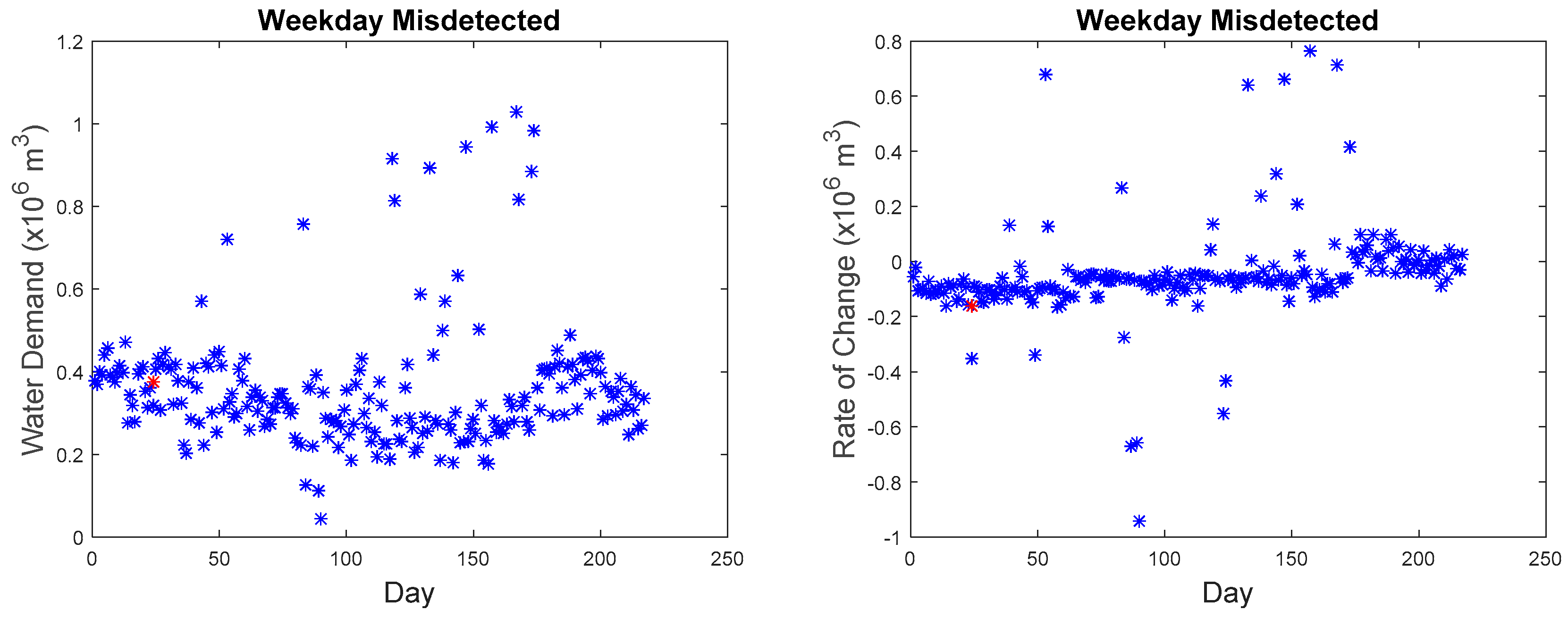
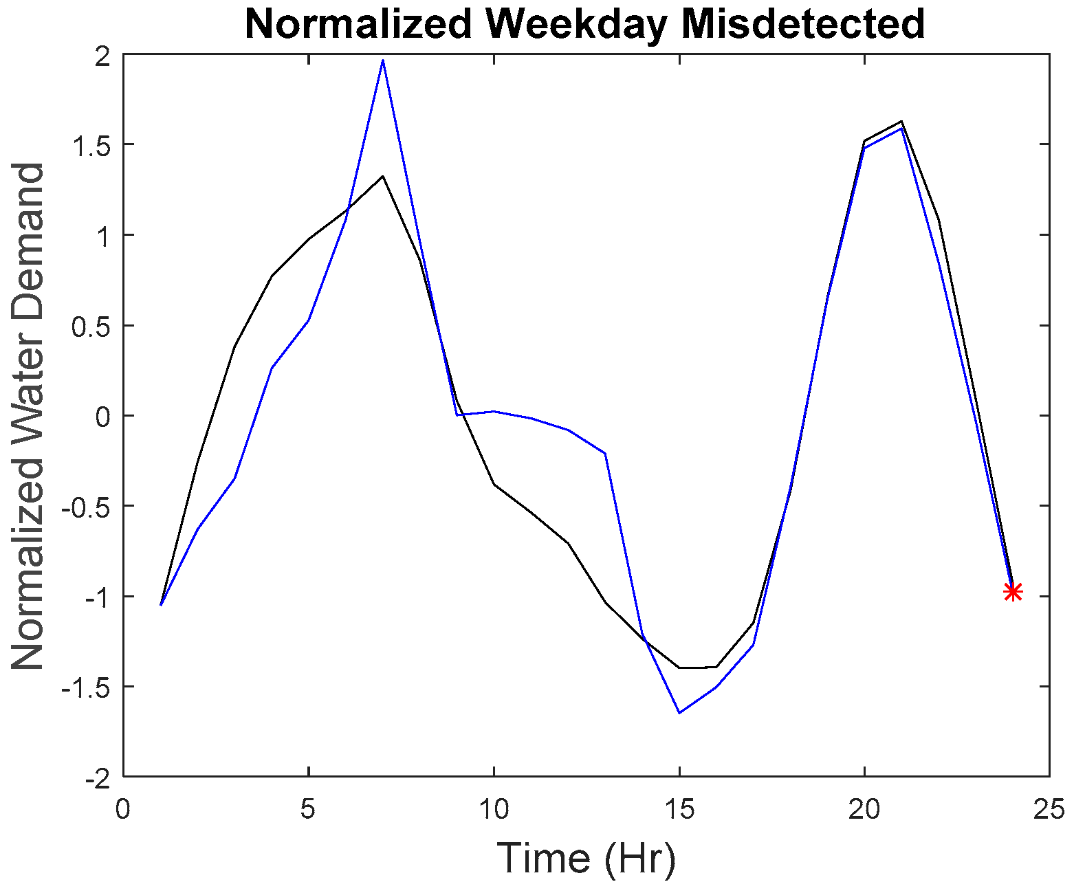
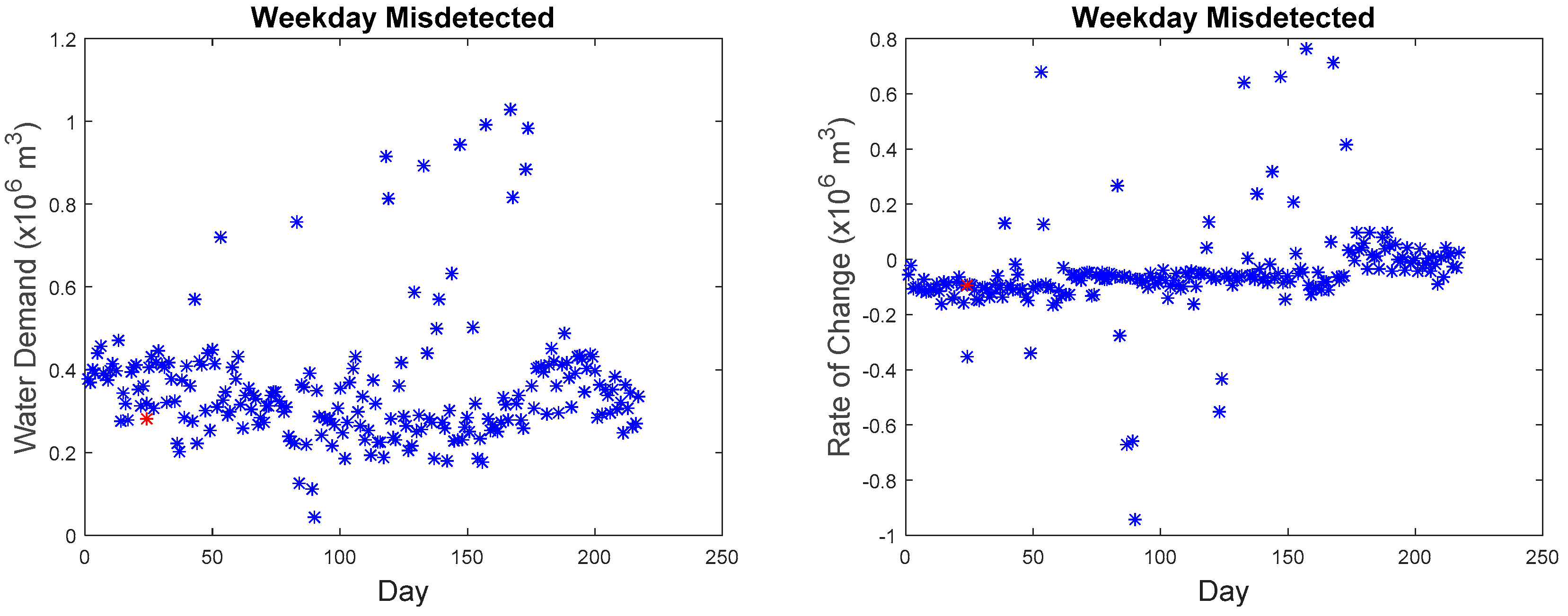
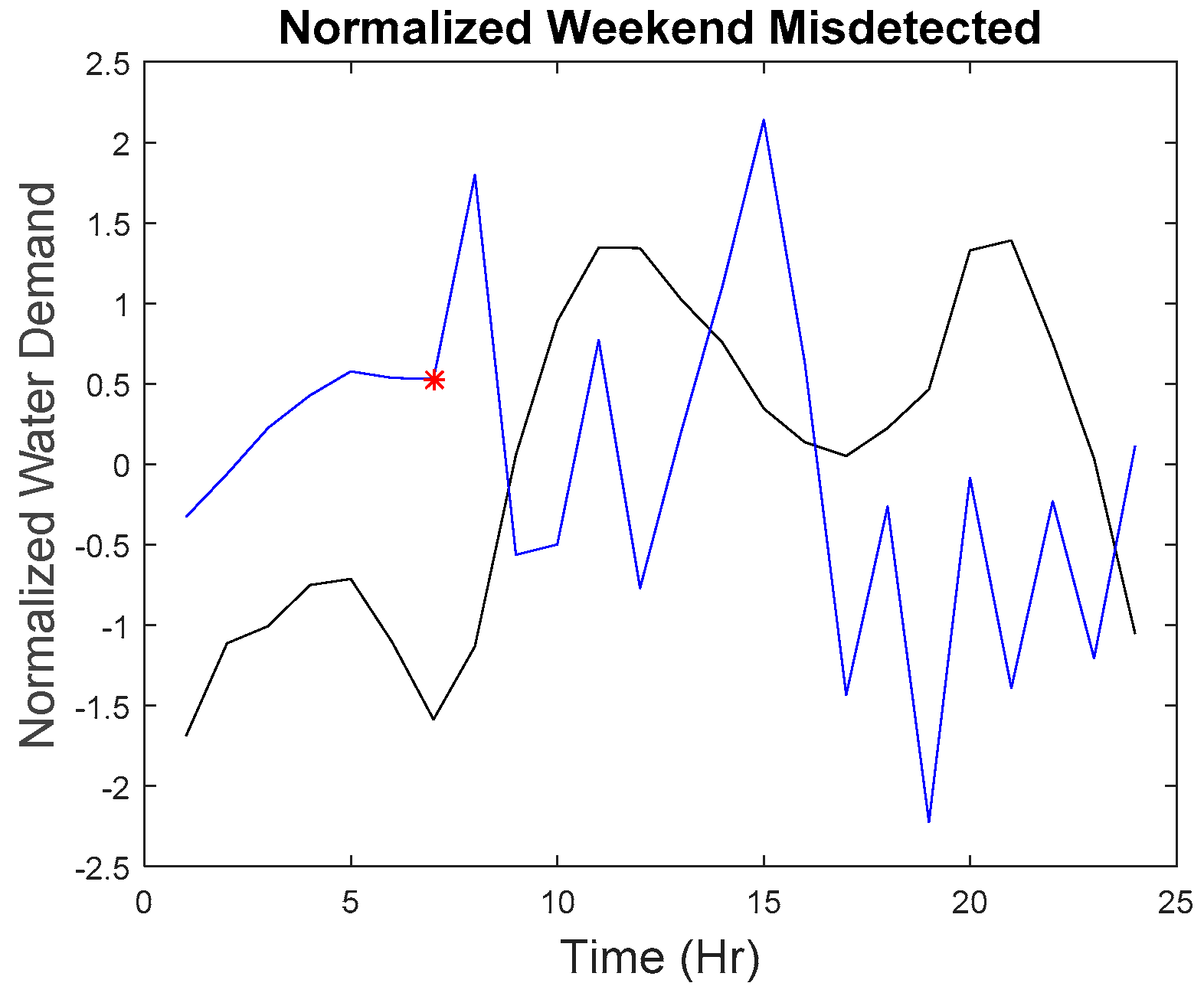
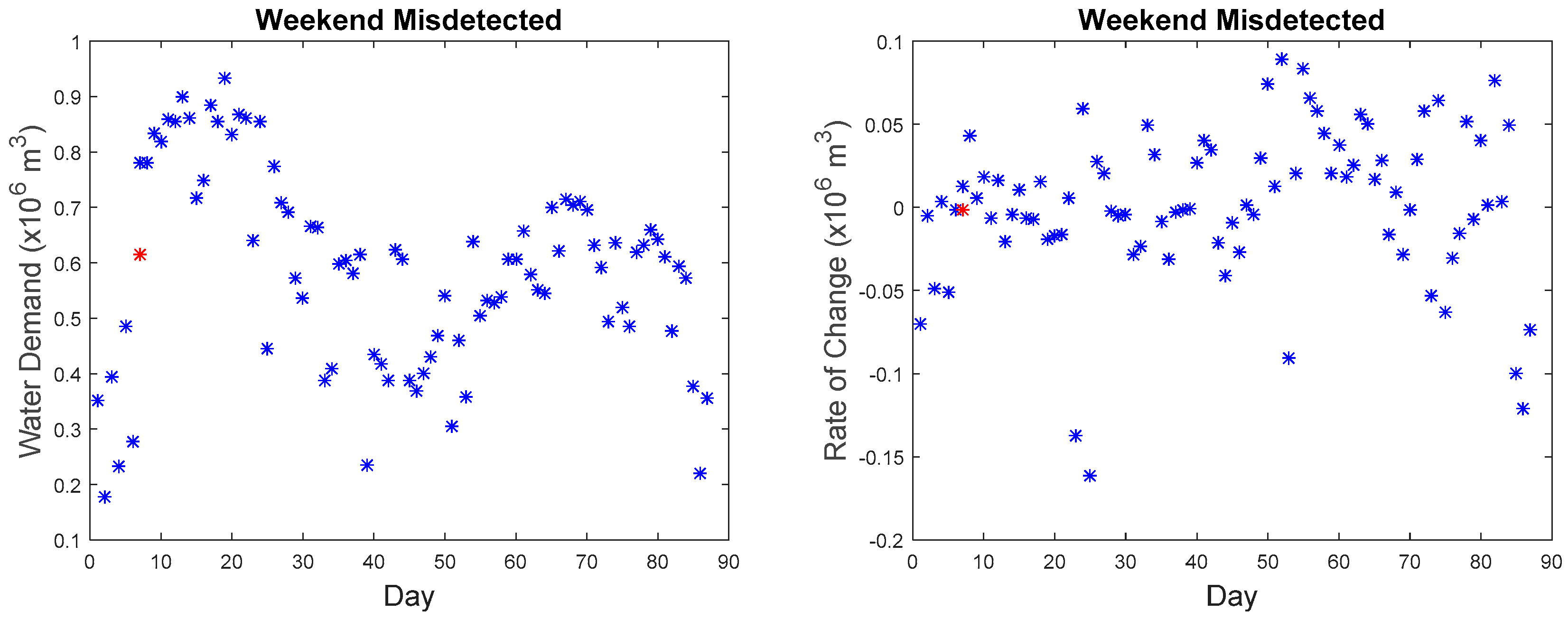
Our microscopic analysis began by plotting the hourly series of the missed detected point with the reference curve. The graph of the anomalous water demand with other water demand as well as the graph of the rate of change with other rates of change at that particular time was also plotted. The red star as shown in Figure 15, Figure 16, Figure 17, Figure 18, Figure 19, Figure 20, Figure 21, Figure 22, Figure 23, Figure 24, Figure 25 and Figure 26 indicate the anomalous point. The black line indicates the reference curve and the blue line indicates the hourly series. The blue star indicates all other points at that particular hour. 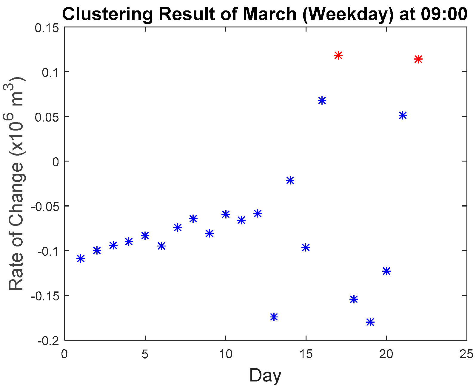Figure 27 presents the clustering results, the red star indicates the member of a minority cluster, and the blue star indicates the member of the majority cluster.

The first missed detected anomaly was found on weekday 09:00. However, the imputed anomaly does not differ much from the normal points. As observed in Figure 15, the overall shape of the curve is quite similar to the reference curve; the water demand does not have a significant difference among other points.

Although as seen in Figure 16, the rate of change is in the anomalous range (−0.15 to −0.2), the rate of change for data points collected at 09:00 in March as seen in Figure 27 are within the range of −0.2 to 0.15 with the majority of the points in the region of −0.05 to −0.1. The second, third, fourth, and fifth anomalous point, which happened on the weekday, also exhibited the same phenomenon where they do not differ significantly from the normal values as seen in Figure 17, Figure 18, Figure 19, Figure 20, Figure 21, Figure 22, Figure 23 and Figure 24. Hence, these points cannot be detected.

The last point on the weekend belongs to a different category as to why it was missed. Although, as seen in Figure 26, the water demand value and rate of change value do not have a big difference as compared to other points, but the series does have a difference with the reference series. However, due to the maximum allowable dissimilarity, the anomaly was not found. By referring to the hourly series from 01:00 to 07:00, it generally adheres to the trend of the reference curve, and the series is within the tolerance of the maximum allowable dissimilarity. The subsequent trend starting at 08:00 shows a significant fluctuation. However, such a trend was detected by the proposed approach as seen in Figure 12. As a result, the proposed approach can sometimes be insensitive to detect a small developing anomalous trend within the maximum allowable similarity. However, the majority of the imputed anomalous points (159 out of 165) were detected successfully.

On the other hand, as the data is unlabeled, detected anomalous trend or other anomalous points could not be verified. Holidays or the festive season could result in an anomalous trend or points and proposed algorithm may classify such event as abnormal.

5. Conclusions

In this paper, a system that tracks the similarity in time, the rate of change, and shape was proposed through the fusion of unsupervised clustering approach and incremental similarity tracking. The proposed approach utilizes data collected from a real DMA using only one month of data and subsequently applied to the remaining nine months of data. The results showed that the proposed approach could detect any anomalous points or trends that deviated from the normal value by examining the water demand value, the rate of change, and shape of the trend at each time step simultaneously.

Such results have validated the claims of real-time detection of the anomalous data point with minimal historical data. The proposed approach has proven the effectiveness of the unsupervised methodology, and through the application of DPMM, it eliminates the need of choosing an optimal cluster number and provides a subtle solution for ‘reserving’ an empty cluster for the future anomaly. The idea of incremental similarity tracking was presented to provide real-time detection of the anomalous trend. Although the results can be insensitive to detect a small developing anomalous trend within the maximum allowable similarity, the majority of the anomalous points were detected successfully.

As the data is unlabeled, other detected anomalous points and trends could not be verified. However, as seen in Figure 10, Figure 11, Figure 12 and Figure 13, such points or trends that were detected were points or trends that do not conform to the usual pattern. Therefore, this system can be a useful tool for preliminary anomaly detection where unusual points or trends can be easily detected and verified through other means. As this case study is targeted towards the water domain, it is possible that such methodology can be applied to other time series that follows a periodic pattern or trend. Similar procedure as discussed in Section 3 can be applied directly on such data as the motivation is to detect anomalous point that does not conform to the usual pattern or trend.

However, to improve the validity and reliability of the proposed algorithm, future research should include testing of this algorithm on labeled data so that another form of accuracy metric such as true or false positive of the anomaly by real problems such as leakage can be verified. Holidays or the festive season should also be taken into consideration for subsequent research as such events can result in a false positive. In addition, future research should also include the detection of an early developing anomaly which can prevent a large amount of water loss.