An Efficient and Structured Procedure to Develop Conceptual Catchment and Sewer Models from Their Detailed Counterparts

Abstract

Modelling flow rates in catchments and sewers with a conceptual, also known as hydrological, approach is widely applied if fast simulations are important. In cases where a detailed hydrodynamic model exists, it is common to start conceptualizing from this detailed counterpart. Unfortunately, no generalized procedure exists, which is surprising as this can be a complex and time-consuming task. This research work proposes a procedure that is validated with two independent combined sewer case studies. The conceptual models provide the targeted results with respect to representation of the flow rates and reduction in the computational time. As the desired performance could be reached for different levels of model aggregation, it is concluded that the conceptual model can be tailored to the points where accurate flow rates need to be predicted. Furthermore, the comparison of the conceptual model results with flow measurements highlights the importance of analyzing and eventually compensating for the limitations of the detailed model.

1. Introduction

The use of lumped conceptual models is widespread in urban drainage modelling where fast calculations are necessary for multiple model evaluations, such as sensitivity or uncertainty analysis and optimization questions [1], or for simulations of long timeseries with complex models, such as integrated models where multiple sub-system models are evaluated at the same time [2,3]. The potential beneficial use of lumped conceptual models was proven with several successful case studies over the last decades. Some examples of their application include sensitivity analysis [4,5], uncertainty analysis [6], real time control (RTC) and model predictive control [7,8] or optimization and integration [9,10,11].

Hydrodynamic routing, also known as distributed flow routing, calculates the flow based on a time and space component using the de Saint-Venant equations [12]. The evaluation of these equations is however computationally demanding and different approaches exist for simplification or emulation of hydrodynamic models [13,14]. Conceptual modelling, also known as hydrological or lumped modelling, is an established approach that uses time alone to calculate the flow rate at a certain location [12]. Conceptual models respect the conservation of mass, but conceptual relations replace the momentum equation, which makes them computationally less demanding [2]. In comparison to hydrodynamic models no flow prediction at intermediate points is possible as the spatial component is lost and several other flow characteristics, such as velocity and water height are no longer calculated. Also, the hydraulic principles that form the basis of conceptual models are that downstream flow conditions do not influence upstream flow conditions. However, in cases where backwater conditions exist, approaches are available to properly approximate those effects [15].

For the development of a conceptual catchment and sewer model, including runoff generation, flow concentration and routing, spatial data representing the catchment and sewer characteristics, as well as flow rate information, have to be available. If a detailed model of the catchments and full hydrodynamic model (de Saint-Venant equations) of the sewer system exist, it is a common approach to use the detailed model as a starting point for conceptualization. This allows incorporating the knowledge already available in the detailed model, thus not imposing a need for extensive collection of flow rate measurement data [7]. For some part of the conceptualization process, semi-automated model layout and calibration tools have been developed to speed up the process [1,16,17]. To the knowledge of the authors, the most complete guideline for conceptual modelling approaches is the Austrian guideline [18], which provides a very good overview of conceptual modelling concepts, including different aggregation strategies for various levels of lumping (available in German only). But even given those tools, a significant amount of time and effort has to be spent developing a conceptual model [1,17]. It is therefore surprising that no general procedure exists to develop conceptualized catchment and sewer models from its detailed counterpart. It was even concluded that a main shortcoming of conceptual modelling is the lack of a formalized generic procedure [19].

Modellers from different disciplines of water system modelling describe that a standardized modelling protocol leads to more efficient and reproducible development of models and makes the process more transparent. Good modelling practice protocols are available for instance in integrated urban wastewater modelling [20], river modelling [21], wastewater treatment modelling [22,23], and river basin and groundwater management [24,25].

This research proposes an efficient and structured procedure to develop conceptual catchment and sewer models from their detailed counterpart (Section 3). The proposed procedure is not automated, but certain sub-steps, such as the development of the aggregated conceptual sewer model [17], could be automated. The conceptualization of special structures, such as pumping stations, retention tanks and flow diversion structures, is not part of the developed procedure, as a general approach to conceptualization is very difficult. Special structures have to be conceptualized on a case-by-case basis. The procedure is applied to two case studies (Ottawa, ON, Canada and Bordeaux, France). Section 4.1 evaluates the performance of the developed conceptual models in comparison to their detailed counterpart. In Section 4.2 the procedure is further tested by evaluating the impact of the level of aggregation on the Ottawa case study. To do so, the initial model, where attention was paid to ensure that catchments were of similar shape and area, is compared to a maximally aggregated model. Section 4.3 challenges the conceptual model of Bordeaux by comparing it to actual flow rate measurements and not only to flow rate data generated by the detailed model.

2. Materials and Methods

2.1. Case Studies

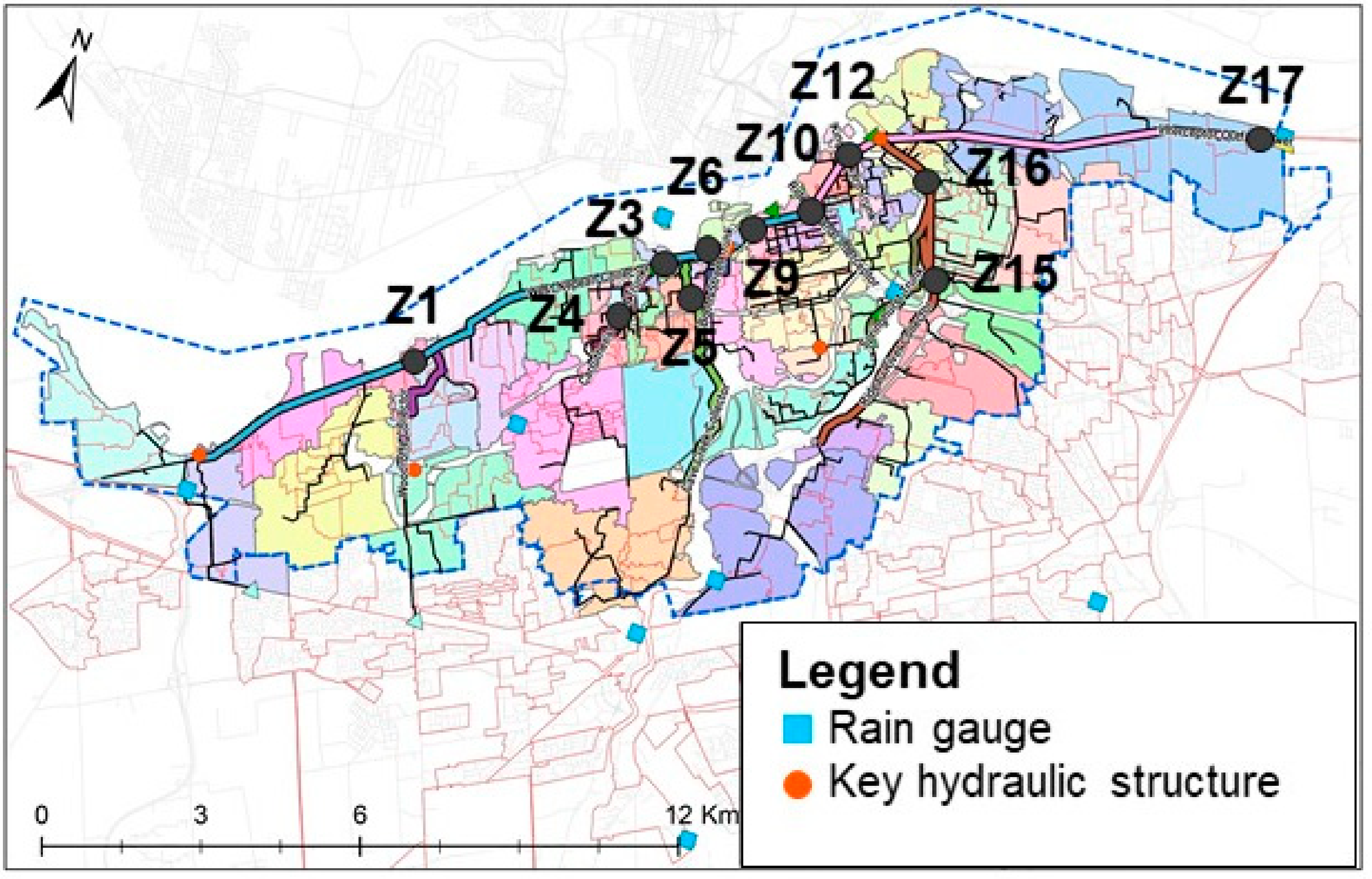
2.1.1. Case Study 1: Ottawa, Canada

The first case study is located in the central urban area of Ottawa, ON, Canada, covering an area of approximately 6400 ha. The catchment contains sanitary, partially separated and combined sewers. In the studied area, rain data from seven rain gauges are available [26]. A map of the considered sewer system is shown in Figure 1.

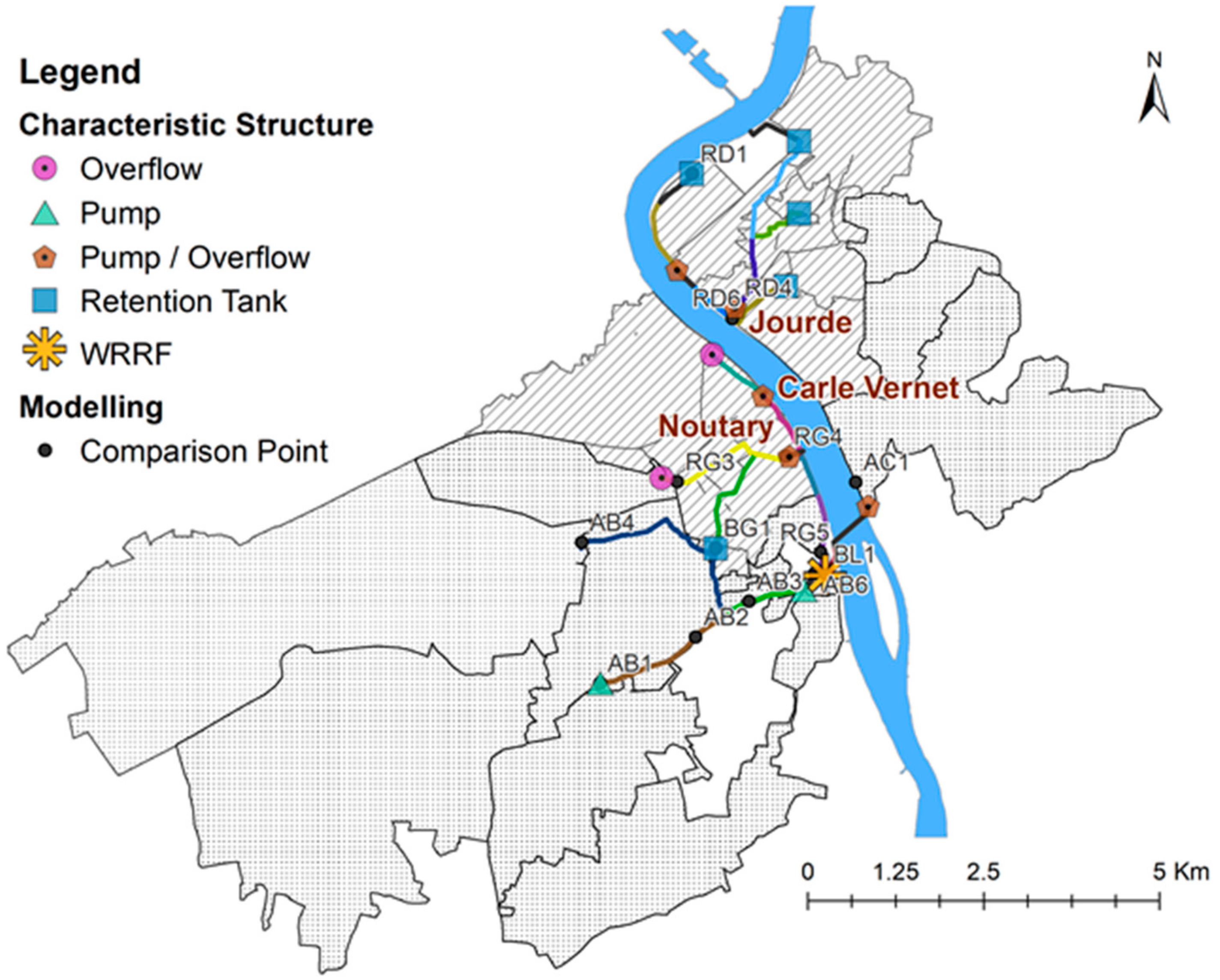
2.1.2. Case Study 2: Bordeaux, France

The second case study is located in the southern part of Bordeaux Métropole, France and covers the catchment of the Clos de Hilde (CdH) wastewater resource recovery facility (WRRF, see Figure 2). The WRRF has four different sewer tributaries, which together cover an area of approximately 8000 ha. The catchment contains both combined and separate sewer systems. Rain data is available for four rain gauges and in contrast to the first case study, flow rate measurements are also available and provided by the local utility. The relevant flow rate measurements are located at the four different tributaries of the WRRF and the pumping stations Jourde, Carle Vernet and Noutary (see Figure 2 for the locations of the WRRF and pumping stations).

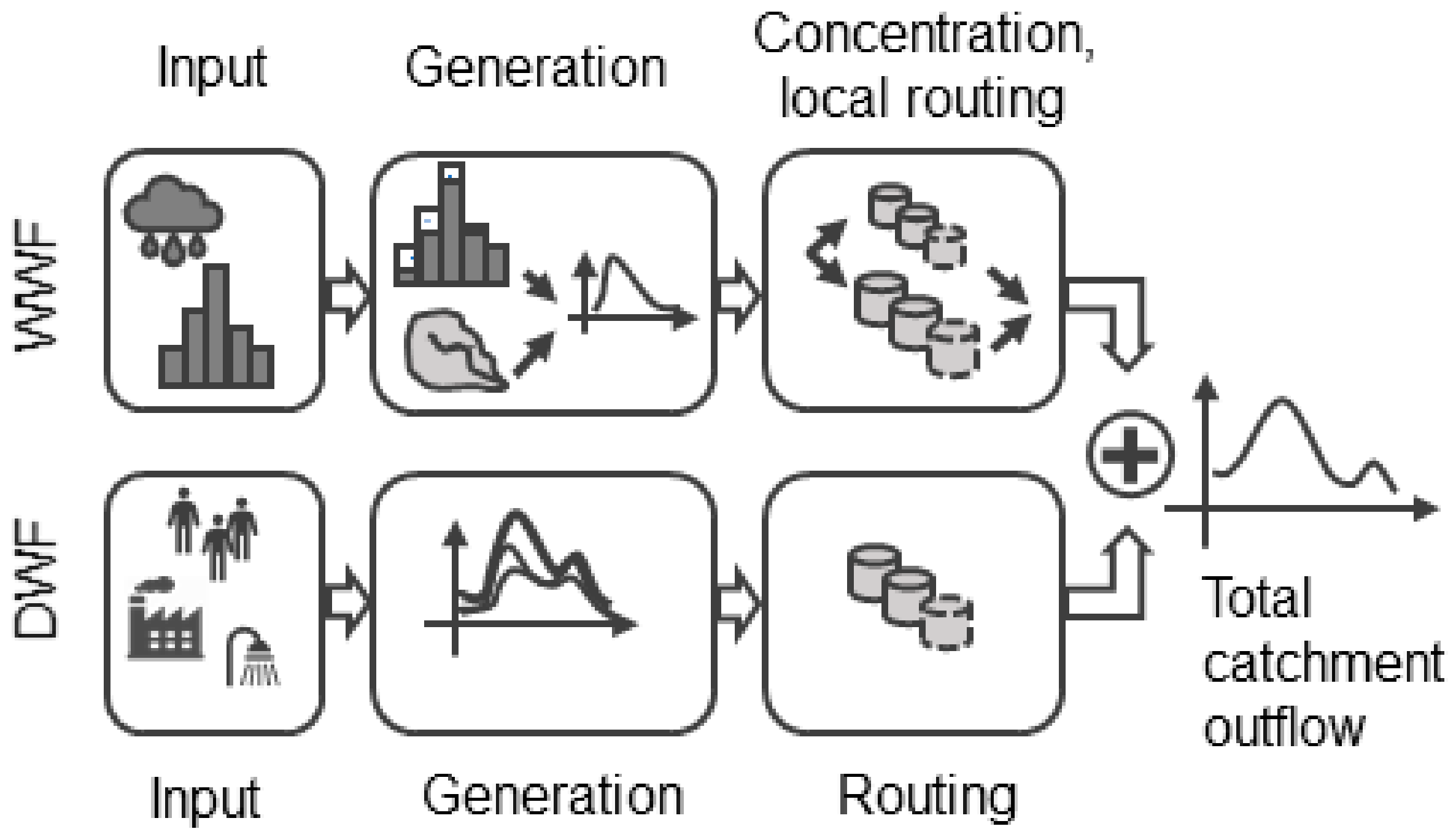
2.2. Modelling Approach and Software

The catchment model is based on the KOSIM catchment model implemented in the software WEST (DHI, Horsholm, Denmark) [27]. The model couples a module for wet weather flow (WWF) and a module for dry weather flow (DWF), as indicated in Figure 3. In comparison to the original KOSIM-WEST model, the WWF can be split into fast and slow flow concentration and local routing through a series of reservoirs to represent the fast and slow responses characteristics of inflow and infiltration responses, respectively [26]. As conceptual catchments are generally aggregated over several detailed catchments, this process represents both flow concentration and routing through the local sewer network that is no longer explicitly modelled. Inputs to the DWF module are the number of people equivalents and their average wastewater generation rates, as well as the average wastewater production by local industry. In comparison to the original KOSIM-WEST model, the DWF is also routed with a series of linear reservoirs representing the local sewer network [26].

The conceptual model of the sewer is based on the reservoir in series approach, also known as a cascade of reservoirs. Equation (1) represents the principle of mass conservation, which requires the difference of the inflow $Q_{\mathrm{in}}$ and outflow $Q_{\mathrm{out}}$ to be equal to the change of storage volume $V\left(t\right)$ [12]. Equation (2) relates the outflow $Q_{\mathrm{out}}$ to the storage volume $V\left(t\right)$ and the storage constant of the reservoir $k$, also known as residence time [12].

If the value of the constant $p$ equals one, Equation (2) corresponds to a linear reservoir, otherwise it is a non-linear reservoir [12]. For both approaches, methods exist to determine the reservoir parameters from the detailed model. Euler [28] adapted the Kalinin-Miljukov method to define the linear reservoir parameters from the pipe characteristics. An alternative method to determine the parameters is the Muskingum method [12]. In the non-linear case the parameters can also be defined using the pipe characteristics from the detailed model, maximum flows and volume-outflow gradients [29]. To approximate backwater phenomena in conceptual modelling, an approach using a sequence of splitter and combiners has been developed and tested for the linear reservoir model [15].

$$\frac{\partial V\left(t\right)}{\partial t}=Q_{\mathrm{in}}\left(t\right)-Q_{\mathrm{out}}\left(t\right)$$

(1)

$$Q_{\mathrm{out}}\left(t\right)=\frac{1}{k}V{\left(t\right)}^{1/p}$$

(2)

All modelling and simulation work was performed utilizing the software WEST (DHI, Horsholm, Denmark), which is a general modelling and simulation environment [30].

2.3. Model Performance Criteria

The model performance criteria chosen for this study are the percent volume error (PVE) in Equation (3), percent error in peak (PEP) in Equation (4) and the Nash-Sutcliffe efficiency (NSE) in Equation (5). The PVE, also known as the percent bias, measures the overall adequacy between predicted ($P_i$) and observed ($O_i$) data. The PEP characterizes the difference between the observed peak ($\max \left(\left\{O_i\right\}\right)$) and the modelled peak ($\max \left(\left\{P_i\right\}\right)$) for a single event but does not evaluate the timing of the peak. The NSE compares the squared residuals with the squared residuals a model written as the mean of the data ($\overline{O}$) would create. The optimal value equals one, zero means that the model is equally good as a mean value model and a negative value means that the model is performing worse than the mean value of the observations. Due to the squared nature of the criterion, it compares to the well-known Root Mean Square Error (RMSE) model performance criterion, used in other disciplines. This criterion is sensitive to extreme values [31].

$$\mathrm{PVE} =100\frac{{\sum }_{i=1}^n\left(O_i-P_i\right)}{{\sum }_{i=1}^n{O}_i}$$

(3)

$$\mathrm{PEP}=100\frac{\max \left(\left\{O_i\right\}\right)-\max \left(\left\{P_i\right\}\right)}{\max \left(\left\{O_i\right\}\right)}$$

(4)

$$\mathrm{NSE}=1-\frac{{\sum }_{i=1}^n{\left(O_i-P_i\right)}^2}{{\sum }_{i=1}^n{\left(O_i-\overline{O}\right)}^2}$$

(5)

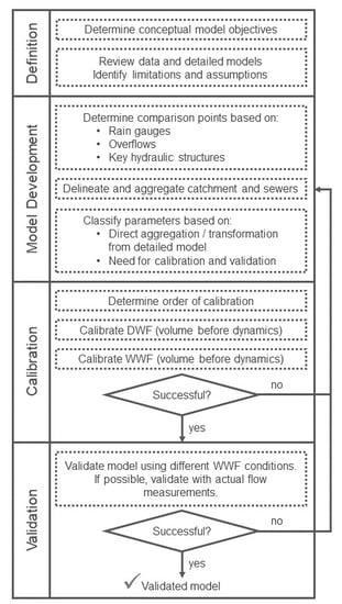
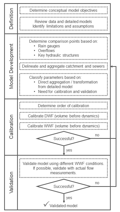
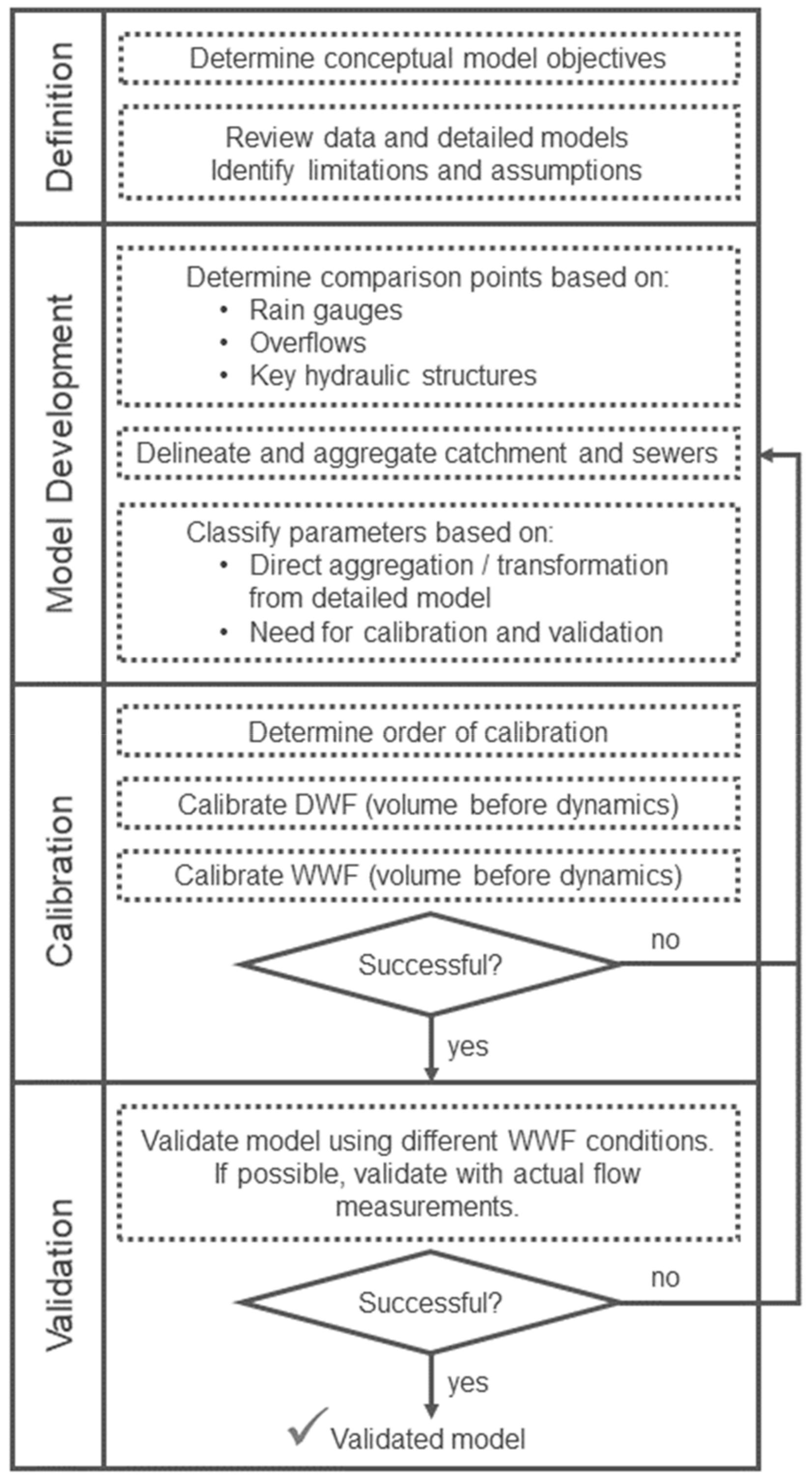
3. Proposed Methodology

The proposed procedure to develop a conceptual model from its detailed counterpart consists of four main stages (Figure 4): Project definition, model development, calibration, and validation. Each of the stages will be explained in more detail in a dedicated sub-section.

3.1. Project Definition

In the stage of the project definition, the first step is to determine the conceptual model’s objectives. These objectives usually reveal on the one hand a certain need of model performance and on the other hand the need of fast calculations, for example for sensitivity or uncertainty analysis or model predictive control. A measure for calculation time is the speed-up factor that needs to be attained for a case study, which is calculated by dividing the simulation time of the detailed model over the time of the conceptual model. The objectives determine whether the development of the conceptual model is an appropriate solution.

The second step is the review of the available data and the detailed hydrodynamic model from which the conceptual model can be developed. The quality of those data and the detailed model have to be assessed. Special attention should be given to the purpose for which the detailed model was built. This influences the limitations and assumptions of the detailed model and therefore also of the conceptual model. Depending on the objectives of the conceptual model, simplifications of the detailed model might be considered to facilitate conceptualization. Possible simplifications affect hydraulic structures where complexity can be reduced, for instance by replacing complex hydraulic relationships and/or RTC rules by simplified overflow structures.

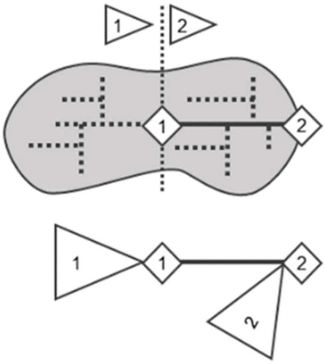
3.2. Model Development

When developing a conceptual model, it is crucial to identify the comparison points, i.e. the points where the conceptual model should predict accurate flow rates and is therefore compared to the detailed model. To do so, it is important that locations of rain gauges, overflows and key hydraulic structures are known. Because conceptual models only predict flow rates at the outlet of a catchment or sewer conduit but not within, no aggregation of catchments and sewers should take place over the comparison points. The selected comparison points therefore have to be calibrated and validated with a corresponding point in the detailed model.

The next step is the delineation and aggregation of catchments and sewers in accordance with previously identified comparison points. The delineation of catchments and sewers has to be carried out simultaneously as they are directly linked. Figure 5 illustrates a simple sewer system and its conceptualization. In the example sewer system, two points are identified as comparison points where flow rates have to be predicted. The illustration shows that the local sewers (dotted lines) are represented as sewer conduits in the detailed model. In the aggregated conceptual model, however, they are no longer represented as a sewer conduit model but are incorporated in the catchment model. Only the main sewer trunk between comparison point 1 and 2 is represented in a specific sewer conduit model. Special attention must be paid to catchments through which a conceptual sewer flows as the parameters of the catchment and the sewer model cannot be calibrated independently at the downstream comparison point. In Figure 5, this situation corresponds to comparison point 2, where the flow rate at this point represents both the flow from the sewer conduit and catchment 2. The parameters of the sewer model can be identified by using the methods described in Section 2.2. Therefore, the flow rate at point 2 can be used to calibrate and validate the catchment parameters of catchment 2 after having calibrated and validated catchment 1. It might be that structural properties of the detailed catchment models are too different and do not allow for aggregation. However, if possible, it is suggested that only one conceptual catchment model is calibrated per comparison point to avoid overparameterization. The catchments have therefore to be delineated accordingly.

The conceptual catchment and sewer models have to be parametrized in the next step. The parameters that can be directly parameterized depend on the model structure of both the detailed and the conceptual model. A comparison of the modelled processes will reveal the parameters that can be directly aggregated or translated from the detailed to the conceptual model and which parameters need calibration and validation. The illustration of the catchment model in Figure 3 shows typical model assumptions for input and generation of both WWF and DWF. It seems inherently clear that the parameters related to model input can usually be aggregated directly from the detailed model, e.g. if a conceptualized catchment contains several detailed catchments, the total person equivalents or effective area of the conceptualized catchment corresponds to the sum of the person equivalents, respectively the effective area, of the detailed catchments. The parameters regarding flow concentration and routing, however, will usually need calibration and validation as no direct translation is possible. Figure 3 shows that the concentration and routing module of the conceptual model differs from the detailed model as the concentration and routing processes are lumped together in the conceptual model (see also Figure 5). The parameters of the conceptual sewer model, representing the routing in the main sewer trunks, can be estimated using the established methods mentioned in Section 2.2 such as the Kalinin-Miljukov method [28], as all the necessary pipe characteristics are available from the detailed model.

3.3. Calibration

For the calibration of a conceptual model from a detailed model, two approaches are possible. The first is the parallel calibration of all sub-models [21]. For each of the conceptual sub-models the detailed model results serve as input at the upstream comparison point. The parameters of the conceptual model are then calibrated at the downstream comparison point by fitting to the detailed model output. This allows independent calibration of all sub-models, which thus permits parallelisation of the calibration task. The second approach is the sequential calibration of the conceptual model, where the output of the previously calibrated upstream conceptual model serves as input to the conceptual model to be calibrated, and not the simulation results of the detailed model. For the proposed procedure, the second approach is adopted, as this approach allows for correction of inevitable model structure errors that occur during conceptualization. Even though the performance of each sub-model might be smaller due to the substitution of the detailed model’s input with the upstream conceptual model, it is assumed that the overall performance at the downstream emission point is better, since upstream errors can be compensated for.

The order in which the parameters are calibrated is important and should be established prior to performing a calibration, as this will ensure that upstream model parameters are calibrated before the downstream parameters. In Figure 5, comparison point 1 is a first order comparison point, as it is further upstream, whereas comparison point 2 is a second order comparison point. Assigning a calibration order for each comparison point has also the effect that it allows for parallel calibration of comparison points with the same order of calibration and therefore speeds up the calibration process.

Once the calibration order is identified the actual calibration is performed. If the catchment model is not known to the modeller, it is suggested to carry out a sensitivity analysis of the catchment model prior to calibration to determine the impact of the available model parameters. The calibration is first carried out for DWF and then for WWF, respecting the calibration order in both cases. For both DWF and WWF, the flow volume is calibrated before the flow dynamics. The previous step identified the parameters that can directly be translated from the detailed to the conceptual model. If the input and generation parameters can be translated directly, volume calibration is not necessary, but validation is recommended. The concentration and routing parameters representing the dynamics of the conceptual catchment model, however, are to be calibrated. Depending on the objective of the conceptual model, different performance criteria can be selected to assess the goodness of fit between the detailed and the conceptual model, see also Section 2.3. If the attained model calibration performance cannot be reached, it is suggested to go back to the previous stage of model development and refine the structure of the model.

3.4. Validation

In the last stage, the conceptual model is validated using a different rain time series. The rain data are used as an input to both the detailed model and the conceptual model. Comparing the flow rates at the identified comparison points with the chosen performance criteria will either validate the model or reveal that a recalibration of the conceptual model is necessary. If flow rate measurements at some points are available, it is strongly suggested to also validate the conceptual model with actual flow rate measurements. If the model validation is not successful it is suggested to go back to the stage of model development and refine the model structure.

4. Results

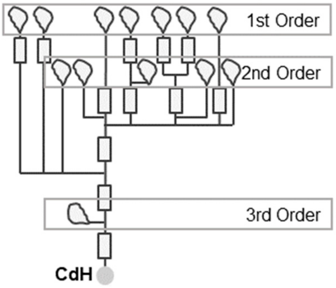
4.1. Developed Conceptual Models

The first stage of the project definition is summarized for both case studies in

Table 1. Project definition of case studies. Objectives of conceptual models, detailed models and available data.

Step	Ottawa	Bordeaux
Objectives conceptual model	Fast conceptual model for later extension to an integrated model (including WRRF). Simulation time of a rain event < 1 min. Calibration: NSE > 0.8 Validation: NSE > 0.65	Fast conceptual model valid over a wide range of conditions to be extended with a water quality model. Simulation time of a rain event < 1 min. Calibration: NSE > 0.8 Validation: NSE > 0.65
Detailed models	SWMM 5 model (United States Environmental Protection Agency), built in 2013 to evaluate pipe capacities and overflows for large storm events (e.g. 100-year return period).	Mike Urban model (DHI, Horsholm, Denmark), built in 2012 to evaluate pumping capacities and overflows under WWF conditions for current and future scenarios (10 to 20 years).
Available data	7 rain gauges	4 rain gauges and 8 flow measurements

.

To identify the comparison points, the location of the rain gauges, overflows, and key hydraulic structures are indicated in Figure 1 for Ottawa and Figure 2 for Bordeaux. The chosen comparison points are shown in the same figures. The input and generation sub-models of the catchment were parametrized by aggregation and translation of the detailed model information. The sewer routing parameters were calculated for both cases by using the Kalinin-Miljukov method [28] mentioned in Section 2.2. The flow concentration and routing parameters in the catchment could not be derived from the detailed model and are therefore calibrated and validated in the next stage.

As a first step in the calibration stage, the calibration order was determined for both case studies. This process is illustrated in Figure 6 for one of the tributaries of the Bordeaux case study. Catchments of the same order of calibration were calibrated in parallel. Following the procedure, the models were first calibrated for DWF and then for WWF. The calibration procedure applied was a grid search, where the best performing set of parameters was chosen if the performance objectives were met. Otherwise the grid was refined. If this did not lead to the desired results, the model structure had to be adapted. The summary of the results given in

Table 2. Summary calibration and validation results. The full calibration and validation results can be found in Table A1 and Table A2 for Ottawa and Bordeaux, respectively.

Performance Indicator	DWF Calibration	WWF Calibration	WWF Validation
Ottawa Model V1
Average NSE	1.00	0.96	0.95
Range NSE	0.99–1.00	0.89–0.99	0.84–1.00
Bordeaux
Average NSE	0.93	0.95	0.87
Range NSE	0.84–1.00	0.84–1.00	0.71–0.94

shows that the calibration objective is met for all comparison points. The full results are provided in

Table A1. Performance Ottawa case study. Calibration and validation results of both the less aggregated (V1) and the maximally aggregated conceptual model (V2) in comparison with the detailed model.

Comp Point	DWF Calibration					WWF Calibration					WWF Validation
	Average Flow (l/s)	Peak Flow (l/s)	PVE (%)	PEP (%)	NSE	Event Volume (103 m3)	Peak Flow (l/s)	PVE (%)	PEP (%)	NSE (-)	Event Volume (103 m3)	Peak Flow (l/s)	PVE (%)	PEP (%)	NSE (-)
Ottawa Detailed Model
Z1	246	307				101	1080				90	880
Z3	570	683				261	2738				229	2106
Z4	192	273				98	1239				83	1735
Z5	112	146				67	805				55	1161
Z6	683	825				328	3539				284	2628
Z9	939	1124				459	4708				401	4833
Z10	977	1171				475	4880				415	4662
Z12	1230	1499				615	6910				543	7026
Z15	590	741				314	3684				267	3919
Z16	645	808				349	4104				295	4202
Z17	2004	2388				979	8801				879	8251
Ottawa-Conceptual V1
Z1	248	323	−1	−5	1.00	107	1080	−6	0	0.97	100	979	−11	−11	0.95
Z3	561	689	2	−1	1.00	268	2738	−3	0	0.99	253	2474	−11	−17	0.97
Z4	191	274	1	−1	0.99	98	1167	1	6	0.96	91	1011	−9	42	0.84
Z5	111	151	1	−3	1.00	66	808	0	0	0.97	55	604	0	48	1.00
Z6	672	837	2	−1	1.00	335	3539	−2	0	0.99	308	3016	−9	−15	0.98
Z9	921	1147	2	−2	1.00	466	4729	−2	0	0.91	436	4753	−9	2	0.88
Z10	956	1194	2	−2	1.00	486	4880	−2	0	0.89	452	4880	−9	−5	0.94
Z12	1198	1504	3	0	1.00	615	6936	0	0	0.96	586	6936	−8	1	0.92
Z15	594	723	−1	2	1.00	320	3779	−2	−3	0.99	289	3530	−8	10	0.95
Z16	654	801	−1	1	1.00	365	4404	−5	−7	0.98	329	4037	−11	4	0.99
Z17	1988	2434	1	−2	1.00	984	8801	−1	0	0.99	944	8801	−7	−7	0.99
Ottawa-Conceptual V2
Z1	248	325	−1	−6	1.00	106	1080	−4	0	0.97	98	1002	−9	−14	0.87
Z3	555	694	3	−2	1.00	268	2738	−2	0	0.99	251	2433	−10	−16	0.87
Z4	190	271	1	0	1.00	99	1231	−1	1	0.97	91	1029	−10	41	0.68
Z5	111	146	1	0	1.00	68	852	−2	−6	0.98	62	650	−13	44	0.77
Z6	667	831	2	−1	1.00	335	3539	−2	0	0.99	313	3080	−10	−17	0.86
Z9	913	1127	3	0	1.00	467	4643	−2	1	0.95	442	4751	−10	2	0.74
Z10	949	1178	3	−1	1.00	486	4880	−2	0	0.92	458	4880	−10	−5	0.74
Z12	1194	1495	3	0	1.00	615	6936	0	0	0.98	591	6936	−9	1	0.80
Z15	591	725	0	2	1.00	319	3711	−1	−1	0.99	286	3555	−7	9	0.87
Z16	652	803	−1	1	1.00	363	4272	−4	−4	0.99	326	3974	−10	5	0.83
Z17	2003	2444	0	−2	1.00	986	8801	−1	0	0.99	947	8801	−8	−7	0.91

for Ottawa and

Table A2. Performance Bordeaux case study. Calibration and validation results of the conceptual model in comparison with the detailed model.

Comp Point	DWF Calibration					WWF Calibration					WWF Validation
	Average Flow (l/s)	Peak Flow (l/s)	PVE (%)	PEP (%)	NSE	Event Volume (103 m3)	Peak Flow (l/s)	PVE (%)	PEP (%)	NSE (-)	Event Volume (103 m3)	Peak Flow (l/s)	PVE (%)	PEP (%)	NSE (-)
Bordeaux-Detailed
AB1	42	49				11.74	192.23				14	375
AB2	60	69				16.35	229.67				19	431
AB3	142	162				39.81	558.11				46	1072
AB4	58	67				16.64	274.78				20	538
AB6	163	186				45.07	581.02				52	1101
AC1	9	12				3.05	90.37				4	176
BL1	22	26				6.05	55.64				7	96
RD1	9	11				3.67	441.28				5	979
RD4	56	65				21.37	1114.45				30	2608
RD6	34	39				17.84	1568.53				31	3390
RG3	124	130				37.51	448.22				42	563
RG4	163	174				58.36	2470.28				76	4898
RG5	439	491				119.03	775.66				123	820
BG1	5	6				2.58	383.10				4	850
Bordeaux-Conceptual
AB1	42	48	0	−1	0.98	11.62	200.10	−1	4	0.97	14	491	5	31	0.91
AB2	60	69	0	0	1.00	16.28	241.06	0	5	0.98	20	570	5	32	0.90
AB3	142	162	0	0	0.97	39.77	559.35	0	0	0.99	49	1316	7	23	0.93
AB4	58	66	0	−1	1.00	16.81	274.88	1	0	0.99	22	667	11	24	0.88
AB6	163	186	0	0	0.97	45.00	579.03	0	0	0.99	55	1334	6	21	0.93
AC1	9	12	0	−4	0.99	2.97	70.00	−3	−23	0.92	4	186	7	6	0.79
BL1	22	26	0	−1	0.99	5.93	58.06	−2	4	0.92	7	124	1	29	0.91
RD1	9	11	1	0	0.91	3.38	434.36	−8	−2	0.96	6	1282	3	31	0.94
RD4	57	67	2	3	0.94	22.06	1226.26	3	10	0.86	35	3266	16	25	0.71
RD6	34	38	−2	−1	0.90	18.29	1671.09	3	7	1.00	36	4747	15	40	0.91
RG3	124	132	0	2	0.84	36.71	450.00	−2	0	0.92	43	450	2	−20	0.72
RG4	163	177	0	2	0.84	57.49	2769.44	−1	12	0.99	83	7271	10	48	0.88
RG5	442	478	1	−2	0.84	118.37	765.85	−1	−1	0.84	123	770	0	−6	0.88
BG1	5	6	0	2	0.89	2.43	396.42	−6	3	0.97	5	1169	11	38	0.89

for Bordeaux. For the fourth and last stage (model validation), a summary of the attainment of the objectives is given in Table 2. It shows that the objective for the NSE is met in both case studies. The full validation results can likewise be found in Table A1 and Table A2. The results of the additional criteria for the simulated overall flow volume and peak flow values show that the conceptual model is not performing as well as during the calibration phase. Nevertheless, the values are still considered acceptable for the current case studies.

A summary of the developed models can be found in

Table 3. Comparison of detailed and conceptual model including the calculation time for the detailed and the conceptual model. Note that the conceptual model includes advective transport for water quality components in both cases.

Model		Ottawa		Bordeaux
		Detailed	Conceptual V1	Detailed	Conceptual
Catchments	#	271	52	57	20
Conduits	#	2600	33	783	16
DWF (2 days)	(min)	8.03	0.53	7.64	0.37
Speedup factor		15		21
WWF (3 days)	(min)	30.7	0.63	10.7	0.92
Speedup factor		49		12

, which indicates the number of catchments and sewer conduits for both the detailed and the conceptual models, as well as the calculation time needed for the same flow rate simulations.

The speed-up factor was calculated by dividing the simulation time of the detailed over the conceptual model. It is to be noted that the conceptual model for both case studies already includes advective transport for water quality components in contrast to the detailed model, where this feature was deactivated as these models were never meant to be used for water quality. Nevertheless, a speed-up factor of over 10 could be reached for all studied flow conditions. The objective of simulating a WWF event within one minute (Table 1) is met for both case studies.

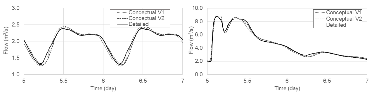
4.2. Level of Aggregation

For the Ottawa case study, the influence of the level of aggregation on model performance was evaluated. For the previously developed model (V1), it was ensured that catchments and sewer conduits were of similar size and that the aspect ratio of the catchments was not too elongated. To do so large catchments and sewers were further divided to avoid a large variation in size and shape. For the further aggregated model V2, this was not considered anymore. This means that, with model V2, the maximum level of aggregation for the chosen comparison points was attained. The resulting characteristics of the catchment and sewer sub-models of the two different aggregation levels are indicated in

Table 4. Comparison model V1 and V2. Characteristics of sub-catchments and sewer conduits and summary of model performance.

Indicator	Attribute	Model V1	Model V2
Catchments	Number of sub-catchments	52	22
	Average/median size	146/102 ha	289/192 ha
	Size range	26–435 ha	26–732 ha
Sewers	Number of conduits	33	17
	Average/median length	1480/1280 m	2580/1490 m
	Length range	100–3000 m	770–7720 m
Speedup factor	DWF (2 days)	15	24
	WWF (3 days)	49	81
Performance	NSE DWF calibration average	1.00	1.00
	NSE DWF calibration range	0.99–1.00	1.00–1.00
	NSE WWF calibration average	0.96	0.97
	NSE WWF calibration range	0.89–0.99	0.92–0.99
	NSE WWF validation average	0.95	0.81
	NSE WWF validation range	0.84–1.00	0.68–0.91

. The more aggregated model V2 has approximately half the number of sub-catchments and sewer conduits than model V1 and thus shows an increased range of size and length parameters.

Sample calibrations of model V1 and V2 in comparison to the detailed model are shown in Figure 7. A summary of both calibration and validation results is given in Table 4, while the full calibration and validation results are provided in Table A1. The validation results indicate that the performance of the model V2 is generally lower, but the validation objective for the NSE (NSE > 0.65) is met at all comparison points. The observation that the dynamics of the flow are generally a little less well represented in the model V2 makes sense, as the further aggregation results in a loss of resolution.

The results of the comparison of the simulation times between both levels of aggregation are also summarized in Table 4. As expected, the further aggregated model V2 is faster than V1, using approximately 2/3 of the simulation time of model V1.

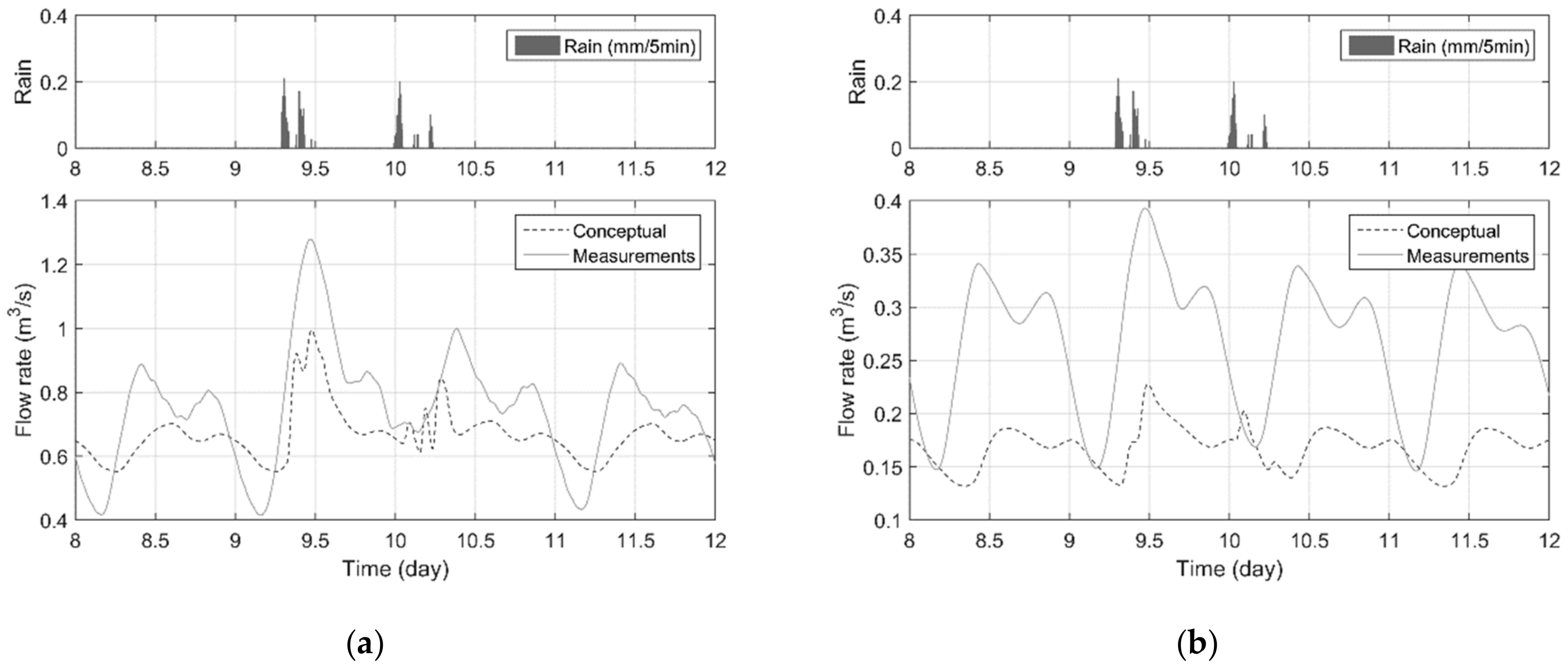
4.3. Comparison of Conceptual Model with Actual Flow Rate Data

As mentioned in Section 4.1, flow rate measurements are available for the Bordeaux case study. The model can thus be compared to actual measurement data and not only to simulation results of the detailed model. This was first done without any further model parameter adjustments after validation with the detailed model and is thus a true validation with respect to the model’s capability to represent reality. Figure 8 shows the total influent rate at the WRRF CdH inlet (a) and one of the four tributary branches (b) for 9–13 May 2017. From the left-hand side illustration, it can be concluded that the overall average DWF (DWF volume) is approximately correct, but that the dynamics are not well represented (dry weather day 8). The WWF, as such, seems underestimated (wet weather days 9–10) but this, as later will be demonstrated, is mainly due to the errors in the DWF. Furthermore, observations at one particular tributary to the WRRF CdH (right-hand side) shows that not only the dynamics do not match, but the average DWF flow for this tributary is clearly underestimated.

Table 5. Comparison of conceptual models with all available actual flow rate measurements. The location of the flow rate measurements is indicated in Figure 2. First the conceptual model built using the detailed model only is compared to the measurements and then the conceptual model with measurement based recalibrated DWF is compared to the measurements.

Comparison Point	Measured	Conceptual (Calibrated on Detailed Model Only)				Conceptual (DWF Recalibrated on Measurements)
	Vol.	Vol.	PVE	PEP	NSE	Vol.	PVE	PEP	NSE
	(103 m3)	(103 m3)	(%)	(%)	(-)	(103 m3)	(%)	(%)	(-)
CdH total	259	231	−11	−22	0.31	247	−5	−2	0.80
CdH Tributary 1	93	58	−37	−42	−2.47	92	−1	2	0.85
CdH Tributary 2	150	162	8	−10	0.59	139	−7	−3	0.69
CdH Tributary 3	9	8	−14	−25	−0.47	10	9	5	0.65
CdH Tributary 4	7	3	−56	−66	−1.99	6	−13	−24	0.72
Jourde Outflow	40	41	2	−16	0.70	38	−7	5	0.52
Jourde Overflow	0	3	n.a.	n.a.	n.a.	2	n.a.	n.a.	n.a.
Carle Vernet Outflow	48	61	26	−18	−0.10	46	−5	−18	0.67
Noutary Inflow	61	59	−2	−17	0.44	55	−10	−12	0.60

summarizes the comparison of the conceptual model results (developed solely based on the detailed model), with the available flow rate measurements, the location of which is indicated in Figure 2. While the overall percentage volume error (CdH total) lies almost within an acceptable 10% error, the errors for each of the individual tributary branches at the inlet of the CdH WRRF are mostly higher. The NSE values demonstrate that the dynamics are poorly represented. Visual analysis of the results indicates that this is mainly caused by the poorly calibrated DWF volume. Good performance under DWF conditions was however never the intention of the detailed model.

As the results indicate shortcomings under DWF conditions, the DWF flow generation in the catchment was recalibrated based on the available flow rate measurements. The parameters changed were the number of people equivalents per catchment and the hourly representation of the daily DWF profile. In addition, it was recognized that some WWF pumping capacities in the system were increased in the time period between the development of the hydrodynamic model (2012) and the collection of more recent flow measurements (2017). These modelled capacities were revised to reflect current maximum pumping capacities.

The results of the recalibrated DWF model are shown in Figure 9 for the same validation period as in Figure 8. The total inflow to the WRRF CdH is shown in (a) while the flows within one of the four tributary branches is depicted on (b). The example shows that both the average flow rate and the dynamics of the hydrograph are matching much better, even though shifts in time can be observed. This is due to the fact that the DWF profile in the conceptual model is now calibrated based on representative data, but the reality is that the system does not have such a consistent DWF pattern at all locations where it is applied in the model. With respect to the WWF response, one can observe that the measurements and the conceptual model simulation results match much better, even though no WWF parameters were changed.

The performance of the conceptual model with the recalibrated DWF contributions in comparison to the available flow measurements is also summarized in Table 5. It can be noted that the recalibration of the DWF greatly improved the performance. However, the conceptual model indicates a small overflow at Jourde, whereas the flow measurements show no such overflow. For this comparison point, the performance criteria could not be calculated (division by zero). However, the actual volume of the overflow reported by conceptual model is comparably small.

5. Discussion

5.1. Development of Conceptual Models

The proposed procedure has been successfully tested with two independent case studies. The results demonstrated that the conceptual models represent the detailed model with the desired level of accuracy and result in considerably shorter simulation times compared to the detailed models.

The question may arise why a conceptual model is better developed from a detailed model and not directly from information about the sewer system and flow rate measurements. The sewer system can be conceptualized with information about its physical properties only (see methods in Section 2.2), but the concentration and routing parameters in the catchment models need to be calibrated and validated on the basis of dynamic flow rate data (see the explanation in Section 3.2). Even though, in general, flow rate measurements can be available at several measurement points throughout the system, they are rarely available at every identified comparison point of the system. A detailed hydraulic model provides the best estimate for this non-existing data. In addition, the detailed model already and inherently contains a significant amount of characteristic data related to the catchment and the sewer system that are needed for the conceptualization, such as the people equivalents per catchment and the physical properties of the sewer pipes. Conceptualization is thus made more efficient by the fact that this data does not need to be collected from other sources.

5.2. Level of Aggregation

Comparing a less aggregated conceptual model (V1) to a maximally aggregated model (V2) for the Ottawa case study showed that model V2 was still able to represent the flow dynamics of the detailed model at the comparison points (Table 4) even though only about half the number of sub-catchments and conduits were used. This means that catchments and sewers can be aggregated to their maximum regarding the comparison points that are to be represented, as long as the special structures’ locations are taken into account. While the number of sub-models was halved, the calculation time dropped only by about one third. This is due to the fixed overhead calculations (e.g. reading input files or plotting), which are independent of the number of sub-models used.

Further model aggregation results in faster simulations and less work to be spent on calibration and validation of the model. However, it comes also at a loss of information at the intermediate points that are no longer simulated and comes with the potential loss of accuracy, if the model structure is oversimplified and rain gauge influence zones are no longer respected.

5.3. Comparison to Flow Rate Measurement Data

Comparing the performance of a conceptual model purely built from a detailed model with real flow rate measurements highlighted two important points. First, the performance of the conceptual model with respect to replicating flow measurements is limited by the performance that the detailed model has with respect to the same flow measurements. This highlights the importance of the project definition stage, where the limitations and assumptions of the detailed model are analysed (see Section 3.1). For the Bordeaux case study, the detailed model was built to evaluate the sewer system under WWF conditions for current and future scenarios (see Table 1). Therefore, average flow rate approximation under DWF conditions was deemed sufficient. The poor performance of the conceptual model with respect to flow rate measurements was therefore caused by the purposeful omission of a DWF calibration and validation of the detailed model. These findings highlight the different purpose for which the detailed model was developed. In addition, it should be noted that the detailed model was developed in 2012, whereas the conceptual model was validated with 2017 flow rate measurements. A part of the discrepancy under DWF conditions might therefore also be caused by additional housing and industrial developments in specific sub-catchments over these 5 years. It is important to note, however, that the sewer network itself was not substantially changed or upgraded during this period.

Second, if the limitations of the detailed model are accounted for and/or rectified (in this case, the recalibration of the DWF model), the conceptual model can perform well in comparison to flow rate measurements without any further adjustments (see Table 5). It can therefore more generally be concluded that if the purpose of the detailed and the conceptual model are not identical, one has to carefully identify the assumptions underlying the detailed model and compensate for them when developing the conceptual model. Nevertheless, the advantages of developing the conceptual model by leveraging the modelling efforts already invested in the development of the detailed model remain very strong.

6. Conclusions

A four-stage modelling procedure was established to develop conceptual catchment and sewer models by maximizing the reuse of information and efforts invested in the development of a detailed hydraulic model. It was applied by different modelers on independent case studies. The procedure resulted in the successful validation of conceptual models for both cases, providing a speed-up factor of 10 to 80 for all comparison conditions. Thus, the conceptual models provide similar results to the detailed models at the selected comparison points but at a simulation rate that is at least ten times faster. It can therefore be concluded that, by applying the procedure, a faster conceptual model can be developed in a structured way. At the same time, it can be concluded that the procedure is sufficiently generic and transportable for application to different case studies. The developed procedure follows similar stages as the Good Modelling Practice protocols reviewed for other disciplines, but is tailored to conceptualization, focusing on aggregation of catchments and sewers.

The study of additional aggregation showed the advantages and disadvantages of further aggregated models. A significant decrease in simulation time (33%) was obtained for an increased level of aggregation, but it was not found to be directly proportional to the level of aggregation. This can be expected for other case studies as well, but the reduction in simulation time is likely to depend on the modelling approach of the conceptual models and certainly also depends on the computational efficiency of the software chosen for both the detailed and the conceptual model.

From the validation of the conceptual model with actual flow rate measurements it could be concluded that the detailed and the conceptual model’s objectives, and with this the modelling assumptions, need to be aligned. If they differ, they reveal where recalibration on actual measurements may be useful. The challenge of the Bordeaux model with actual flow rate data, however, also demonstrated that, if the assumptions of the detailed model are corrected, the conceptual model performs very well without further adjustments.

It is overall concluded that the proposed procedure provides a structured way to use the detailed model to develop the conceptual model. The procedure helps modelers to systematize the modelling process. The suggested procedure therefore improves the current situation in conceptual modelling, for which such a generally applicable procedure was missing.

References

1. Wolfs, V.; Villazon, M.F.; Willems, P. Development of a semi-automated model identification and calibration tool for conceptual modelling of sewer systems. Water Sci. Technol. 2013, 68, 167–175. [Google Scholar] [CrossRef] [PubMed]
2. Achleitner, S.; Möderl, M.; Rauch, W. CITY DRAIN©—An open source approach for simulation of integrated urban drainage systems. Environ. Model. Softw. 2007, 22, 1184–1195. [Google Scholar] [CrossRef]
3. Rauch, W.; Bertrand-Krajewski, J.-L.; Krebs, P.; Mark, O.; Schilling, W.; Schütze, M.; Vanrolleghem, P.A. Deterministic modelling of integrated urban drainage systems. Water Sci. Technol. 2002, 45, 81–94. [Google Scholar] [CrossRef] [PubMed]
4. Gamerith, V.; Neumann, M.B.; Muschalla, D. Applying global sensitivity analysis to the modelling of flow and water quality in sewers. Water Res. 2013, 47, 4600–4611. [Google Scholar] [CrossRef] [PubMed]
5. Vanrolleghem, P.A.; Mannina, G.; Cosenza, A.; Neumann, M.B. Global sensitivity analysis for urban water quality modelling: Terminology, convergence and comparison of different methods. J. Hydrol. 2015, 522, 339–352. [Google Scholar] [CrossRef] [Green Version]
6. Mahmoodian, M.; Delmont, O.; Schutz, G. Pollution-based model predictive control of combined sewer networks, considering uncertainty propagation. Int. J. Sustain. Dev. Plan. 2017, 12, 98–111. [Google Scholar] [CrossRef]
7. Meirlaen, J.; Van Assel, J.; Vanrolleghem, P.A. Real time control of the integrated urban wastewater system using simultaneously simulating surrogate models. Water Sci. Technol. 2002, 45, 109–116. [Google Scholar] [CrossRef] [PubMed] [Green Version]
8. Weinreich, G.; Schilling, W.; Birkely, A.; Moland, T. Pollution based real time control strategies for combined sewer systems. Water Sci. Technol. 1997, 36, 331–336. [Google Scholar] [CrossRef]
9. Bauwens, W.; Vanrolleghem, P.A.; Smeets, M. An evaluation of the efficiency of the combined sewer-wastewater treatment system under transient conditions. Water Sci. Technol. 1996, 33, 199–208. [Google Scholar] [CrossRef]
10. Benedetti, L.; Langeveld, J.; van Nieuwenhuijzen, A.F.; de Jonge, J.; de Klein, J.; Flameling, T.; Nopens, I.; van Zanten, O.; Weijers, S. Cost-effective solutions for water quality improvement in the Dommel river supported by sewer-WWTP-river integrated modelling. Water Sci. Technol. 2013, 68, 965–973. [Google Scholar] [CrossRef]
11. Willems, P. Quantification and relative comparison of different types of uncertainties in sewer water quality modeling. Water Res. 2008, 42, 3539–3551. [Google Scholar] [CrossRef] [PubMed]
12. Maidment, D.R. Handbook of Hydrology; McGraw-Hill: New York, NY, USA, 1993. [Google Scholar]
13. Davidsen, S.; Löwe, R.; Thrysøe, C.; Arnbjerg-Nielsen, K. Simplification of one-dimensional hydraulic networks by automated processes evaluated on 1D/2D deterministic flood models. J. Hydroinform. 2017, 19, 686–700. [Google Scholar] [CrossRef] [Green Version]
14. Machac, D.; Reichert, P.; Albert, C. Emulation of dynamic simulators with application to hydrology. J. Comput. Phys. 2016, 313, 352–366. [Google Scholar] [CrossRef] [Green Version]
15. Vanrolleghem, P.A.; Kamradt, B.; Solvi, A.-M.; Muschalla, D. Making the best of two hydrological flow routing models: Nonlinear outflow-volume relationships and backwater effects model. In Proceedings of the 8th International Conference on Urban Drainage Modelling, Tokyo, Japan, 7–11 September 2009. [Google Scholar]
16. Guo, L.; Tik, S.; Ledergerber, J.M.; Santoro, D.; Elbeshbishy, E.; Vanrolleghem, P.A. Conceptualizing the sewage collection system for integrated sewer-WWTP modelling and optimization. J. Hydrol. 2019, 573, 710–716. [Google Scholar] [CrossRef]
17. Kroll, S.; Wambecq, T.; Weemaes, M.; Van Impe, J.; Willems, P. Semi-automated buildup and calibration of conceptual sewer models. Environ. Model. Softw. 2017, 93, 344–355. [Google Scholar] [CrossRef]
18. Muschalla, D.; Leimgruber, J.; Maier, R.; Tscheikner-Gratl, F.; Kleidorfer, M.; Wolfgang, R.; Ertl, T.; Kretschmer, F.; Sulzbacher, R.M.; Neunteufel, R. DATMOD—Rehabilitation and Adaptation Planning of Small and Medium-Sized Sewer Systems; Bundesministerium für Land- und Forstwirtschaft, Umwelt und Wasserwirtschaft: Wien, Österreich, 2015. (In German) [Google Scholar]
19. Wolfs, V. Conceptual Model Structure Identification and Calibration for River and Sewer Systems. Ph.D. Thesis, KU Leuven, Leuven, Belgium, 2016. [Google Scholar]
20. Muschalla, D.; Schütze, M.; Schroeder, K.; Bach, M.; Blumensaat, F.; Gruber, G.; Klepiszewski, K.; Pabst, M.; Pressl, A.; Schindler, N.; et al. The HSG procedure for modelling integrated urban wastewater systems. Water Sci. Technol. 2009, 60, 2065–2075. [Google Scholar] [CrossRef] [PubMed]
21. Wolfs, V.; Meert, P.; Willems, P. Modular conceptual modelling approach and software for river hydraulic simulations. Environ. Model. Softw. 2015, 71, 60–77. [Google Scholar] [CrossRef] [Green Version]
22. Gernaey, K.V.; van Loosdrecht, M.C.M.; Henze, M.; Lind, M.; Jørgensen, S.B. Activated sludge wastewater treatment plant modelling and simulation: State of the art. Environ. Model. Softw. 2004, 19, 763–783. [Google Scholar] [CrossRef]
23. Rieger, L.; Gillot, S.; Langergraber, G.; Ohtsuki, T.; Shaw, A.; Takacs, I.; Winkler, S. Guidelines for Using Activated Sludge Models. IWA Task Group on Good Modelling Practice; Scientific and Technical Report No. 22; IWA Publishing: London, UK, 2012. [Google Scholar]
24. Refsgaard, J.C.; Henriksen, H.J.; Harrar, W.G.; Scholten, H.; Kassahun, A. Quality assurance in model based water management-review of existing practice and outline of new approaches. Environ. Model. Softw. 2005, 20, 1201–1215. [Google Scholar] [CrossRef]
25. Scholten, H.; Kassahun, A.; Refsgaard, J.C.; Kargas, T.; Gavardinas, C.; Beulens, A.J.M. A methodology to support multidisciplinary model-based water management. Environ. Model. Softw. 2007, 22, 743–759. [Google Scholar] [CrossRef]
26. Pieper, L. Development of a Model Simplification Procedure for Integrated Urban Water System Models—Conceptual Catchment and Sewer Modelling. Master’s Thesis, Université Laval, Québec, QC, Canada, 2017. [Google Scholar]
27. Meirlaen, J. Immission Based Real-Time Control of the Integrated Urban Wastewater System. Ph.D. Thesis, Universiteit Gent, Ghent, Belgium, 2002. [Google Scholar]
28. Euler, G. A hydrological approximation for the calculation of waves in circular pipes. In Wasser und Boden; Heft 2, TU Darmstadt: Darmstadt, Germany, 1983; pp. 85–88. (In German) [Google Scholar]
29. Mehler, R. Combined Sewage Treatment—Process and Modeling; Heft 113; Mitteilungen des Institutes für Wasserbau und Wasserwirtschaft, TU Darmstadt: Darmstadt, Germany, 2000. (In German) [Google Scholar]
30. Vanhooren, H.; Meirlaen, J.; Amerlinck, Y.; Claeys, F.; Vangheluwe, H.; Vanrolleghem, P.A. WEST: Modelling biological wastewater treatment. J. Hydroinform. 2003, 5, 27–50. [Google Scholar] [CrossRef]
31. Hauduc, H.; Neumann, M.B.; Muschalla, D.; Gamerith, V.; Gillot, S.; Vanrolleghem, P.A. Efficiency criteria for environmental model quality assessment: A review and its application to wastewater treatment. Environ. Model. Softw. 2015, 68, 196–204. [Google Scholar] [CrossRef]
Figure 1. Map of the Ottawa case study. The map shows the central sewer area of Ottawa indicating rain gauges and key hydraulic structures as well as the catchments and sewer conduits of the developed conceptual model with the comparison points of the hydrodynamic and conceptual model, indicated by a Z-code (see Section 4.1).
Water 11 02000 g001
Figure 2. Map of the Bordeaux case study. The map shows the Clos de Hilde catchment of Bordeaux with combined (hatched) and sanitary (dotted) sub-catchments of the separate system, the pumping stations with flow rate measurements (Jourde, Carle Vernet and Noutary) as well as comparison points of the hydrodynamic and conceptual model, indicated by a code of two letters and a number (see Section 4.1).
Water 11 02000 g002
Figure 3. Catchment model. Extended KOSIM catchment model implemented in the software WEST (DHI, Horsholm, Denmark) with a dry weather flow (DWF) and wet weather flow (WWF) module. The extension includes the splitting of the WWF in a fast and a slow concentration component and the routing of the DWF.
Water 11 02000 g003
Figure 4. Proposed conceptual modelling procedure. Schema for the proposed procedure for the development of a conceptual model from its detailed counterpart.
Water 11 02000 g004
Figure 5. Conceptualization schema. Schema illustrating a detailed model and its conceptual counterpart with two comparison points resulting in a conceptual model of two catchments and one sewer (inspired by [18]). The labelling of the comparison points indicates the calibration order.
Water 11 02000 g005
Figure 6. Calibration order. Schema of the calibration order for one of the four inlets at the wastewater resource recovery facility (WRRF) of the Bordeaux case study.
Water 11 02000 g006
Figure 7. Sample flow results at selected location for DWF calibration (left-side) and WWF calibration (right-side) for the less aggregated conceptual model (V1) and the maximally aggregated model (V2).
Water 11 02000 g007
Figure 8. Comparison conceptual model with actual flow rate measurements. Comparison of the conceptual model built using the detailed model only with flow rate measurements for the total influent flow rate at the WRRF CdH (a) and one of the four tributary branches (b).
Water 11 02000 g008
Figure 9. Comparison of conceptual model with recalibrated DWF contributions with actual flow rate measurements. Actual flow rate measurements were used to recalibrate the conceptual model for comparison with measured influent flows for the total influent flow rate at the WRRF CdH (a) and one of the four tributary branches (b).
Water 11 02000 g009