Article

Coastal Flooding Hazard Due to Overflow Using a Level II Method: Application to the Venetian Littoral

ICEA Department, Padua University, v. Ognissanti 39, 35129 Padova, Italy
*
Author to whom correspondence should be addressed.
Water 2019, 11(1), 134; https://doi.org/10.3390/w11010134
Submission received: 19 November 2018 / Revised: 13 December 2018 / Accepted: 21 December 2018 / Published: 13 January 2019

Abstract

:
In recent years, marine flooding and its impacts have become a question of growing interest, since coastal areas are the most heavily populated and developed land zones in the world. This paper presents a rapid tool for mapping at regional scale the hazard associated with coastal flooding due to overflow. The tool merges a recently developed numerical model that solves a simplified form of the Shallow-Water Equations and is suited for Graphic Processing Unit (GPU) acceleration, with a Level II reliability method that allows producing hazard maps of inland flooding propagation. The procedure was applied to two stretches of the Venetian littoral, i.e., Valle Vecchia and Caorle, located in the northern Adriatic Sea. The application includes the site descriptions and the resulting hazard maps that show the probability of failure in each point of the coast for a given inland inundation level.

1. Introduction

The EU water flood directive (2007/60/EC) points out the importance of evaluating coastal flooding hazard maps. Under climate change, some authors predicted that sea-levels and subsidence will rise [1] and storm surge intensity will increase [2,3]. Therefore, it is possible that, in the near future, many human infrastructures will be affected by marine flooding and, assuming the coastal population will grow [4], tools for risk mitigations are deemed necessary.
Coastal flooding may be triggered by many causes, possibly in combination: (i) high sea level (and wave run-up) overtopping the artificial dikes/barriers or natural dunes; (ii) breaching of cliffs, dunes or more generally erosion of the coastal defence; (iii) river overflow; and (iv) rain excess or insufficient drainage system. However, it is very complex to account for all these mechanisms. In particular, breaching is very difficult to predict, since it reasonably depends on the (spatially distributed) geotechnical characteristics of the coastal dunes and, for instance, on the presence of vegetation or type of revetment.
In the absence of a complete framework for the assessment of coastal flooding hazard, the maps are frequently based on simple indexes that typically combine topographic information (usually available to the coastal managers within GIS database) to sea level and wave run-up. Many specific open-source tools and approaches have been developed to provide an assessment of the potential flood risk for coastal zone and to support decision-making processes [5,6]. For instance, the National Oceanic and Atmospheric Administration [7] developed a GIS awareness tool to display the resulting inundation from storm surges along the US coastal states vulnerable to hurricanes. Wadey et al. [8] presented a methodology for integrating existing models for the rapid simulation of coastal flood events across a large and varied case study area on the UK south coast. Spaulding et al. [9] developed flood inundation maps for Charlestown (RI) using state of the art, fully coupled high-resolution surge and wave models. In Italy, Aucelli et al. [10] recently studied the inundation hazard and risk in Volturno coastal plain in Campania (Italy). Di Luccio et al. [11] focused on the effect of different run-up lumped formulas on the index for coastal vulnerability assessment of a microtidal beach located along the southern Ionian coast of Calabria (Italy). Di Risio et al. [12] assessed coastal hazard to wave-induced flooding at the national scale. In other cases, the mapping of areas potentially exposed to inundation is carried out by a chain of models (e.g., [13,14]), solving the wave transformation problem in the sea area and the flow propagation in the inland area.
The issue is particularly relevant for the Venetian littoral, where local managers require (possibly GIS-integrated) rapid tools to simulate the coastal flood by means of wave overtopping in an urban area at regional scale. The northern Adriatic coast is subject to rapidly evolving pressures from a range of drivers, including natural and anthropogenic ones: for example, rapid morphological evolution of Po River Delta [15], human-induced subsidence caused by fluid withdrawal [16], and changing wave climate [2]. The study here presented originates from the practical need to fill a gap in the coastal flooding assessment in the Veneto region, until now studied with simplified approaches. The objective of this study was to develop a flood propagation model and to establish a methodology that has the ambition to help the coastal managers and stakeholders in producing flooding hazard maps required under the EU water floods directive.
For the evaluation of the coastal hazard, Lerma et al. [14] compared a traditional approach, based on the simulation of events with given return periods, to a novel empirical method that tries to better define, by analyzing the uncertainties of the hydraulic drivers, the real return period of the flooding event. In the work of Martinelli et al. [17], the failure probability is found following the Level II methodology. They defined in each location the combination of loads that induces a flooding depth larger than a given threshold. The final result is the actual probability that a specific failure mechanism (e.g., overflow) occurs, for an in-erodible topography (e.g., deterministic resistance). The results produced by such models are certainly more rigorous than the traditional approach for the selected failure mode, since they are statistically based. However, they cannot include the expert judgement of the coastal managers. It should be stressed that the maps proposed by this work require an integration before they may be used for coastal management purposes, for instance other failure mechanism and information on the exposed value. Mitigation measures against marine inundation include alert services [18], evacuation procedures [19,20], flood insurance programs [21], structural defences (e.g., dikes and breakwaters [22]), planning options [23], community information and participation [21,24,25], and protection of natural buffer zones (e.g., dunes [26,27]).
This paper includes two main sections and a concluding paragraph. First, the dynamic reduced-complexity model of coastal flooding is briefly described together with the procedure for mapping coastal flooding hazard. The method’s application to two stretches of coast belonging to the Venetian littoral is then presented (Valle Vecchia and Caorle). Lastly, conclusions are drawn.

2. Methodology

2.1. GPU-Based Swallow Water Equation Model

The propagation model is a raster-based inundation model, presented by Favaretto et al. [28,29], that solves for each cell of the domain a simplified form of the Shallow-Water Equations (Equations (1) and (2)) applied in the x and y directions to simulate two-dimensional flow over a raster grid.
w t + q x x + q y y = 0
q ξ t + ( q ξ 2 / w ) ξ = g h ( h ξ + j )
where ξ = x or y. In Equations (1) and (2), h = w + z (w = water depth, z = bed elevation) is the water surface elevation and q ( m 2 / s ) is the discharge per unit width assuming a rectangular channel.
In the momentum equation (Equation (2)), to simplify the equation and to speed up the model, only the more relevant terms are taken into account. The inertial terms are included to avoid overestimation of the fluxes between adjacent cells and to account for the flooding duration. The friction term j is important for the correct simulation of the flow propagation; however, it is linearized, with a coefficient K H that accounts for the linearized turbulent friction flow.
K H = 8 g 3 π Q M A X K s 2 w F 1 / 3
where w F is the maximum available depth through which water can flow between two adjacent cells and it is defined, following [30], as the difference between the highest water free surface in the two cells and the highest bed elevation. Q M A X is the maximum discharge during the sinusoidal oscillation. In practice, the value of Q M A X is assessed as the maximum discharge flowing through the cells.
Forces induced by the advection terms would dominate in presence of small scale features (which generate significant velocity spatial derivatives), but, in absence, bed friction dominates over the advection terms that may therefore be neglected [31].
The final formulation of the momentum equation, only valid where the flow advection is relatively unimportant, becomes:
q ξ t + g w F h ξ + K H q ξ w F 2 = 0
The discretization method implemented is first order in space and time (Euler scheme minimizes memory requirements), and a semi-implicit treatment is used for the friction term to improve stability. The domain coincides with the DTM (Digital Terrain Model), usually subdivided into square cells (area equal to Δ x Δ y ) forming a regular grid. The numerical model is subject to the Courant–Freidrichs–Levy ( C F L ) condition: C F L = V Δ t / Δ x < 1 . To avoid non-physical discontinuities in the flow and to reduce the dispersion error in the numerical scheme, a relaxation technique was used. The discharge q at time t is evaluated in two steps: first, q is obtained on the basis of the balance equation and then q is updated as a weighted average that accounts for the discharge of the neighbouring points. To preserve positivity, the maximum discharge that flows between adjacent cells is limited by a two-step approach. The positive preserving property is crucial when in part of the domain no water is present, or when the water depth is very small, and little oscillations may lead to negative depths, eventually resulting in the simulation to fail [32]. Specifically, if the depth variation Δ h evaluated in a cell is negative (namely, the cell is emptying too much due to a large time step), its absolute value must be less or equal to the current available depth. If it is not, the “negative” volume is subtracted from the spatially connected cells with positive balance to ensure continuity.
Computational efficiency is one of the key issues in the application of raster-based models (or more refined hydraulic models) with Δ x of order 1–5 m. Computational speed depends mainly on grid size and, in fact, dynamic models are often applied to coarse grid only ( Δ x > 100 m), whereas, in this study, the grid cell dimension is Δ x = 1 m. Furthermore, the inundated area evolves throughout the simulation in a manner that is rarely known a priori, meaning that the model domain must be very large to incorporate the flood uncertain extent.
To reduce the model runtime (as suggested in [33,34]), it was decided to write a code suitable for a GPU card to reduce the model run time through parallelization. The code was written in MATLAB and, using the Parallel Computing Toolbox with minimal code changes, the simulation can be run in parallel.
The GPU used to execute the simulation was a Nvidia Tesla K80 (4992 core, 12 GByte memory). GPUs achieve high performance by calculating many results in parallel since each computation is processed by a different core. For very large domains ( 10 8 cells, typical of a regional map), it was found that the GPU time is 2–3% of the CPU (Central Processing Unit) time [28,29].
The overall model consistency was successfully validated through a number of analytical and experimental benchmarks [28,29]. The behavior of the model for very large domains was checked against the analytical solution of the Shallow-Water Equations regarding an oscillatory flow in a parabolic bowl with friction. The numerical ability to simulate wet/dry transitions and the importance of the convective terms were evaluated through a set of comparisons with the experimental investigation of Synolakis [35] for a solitary wave run-up on a simple beach. The flow propagation in a three-dimensional domain was analyzed through a comparison with the experimental investigation of Briggs et al. [36] for solitary wave interaction around a circular island. To prove the model ability to simulate a real case of coastal flooding, an event that occurred at Caorle (VE) in December 2008, documented by videos and reports, was also analysed.

2.2. Procedure for the Assessment of Coastal Flooding Hazard Maps

In the following, a single mechanism is analyzed as responsible for coastal flooding: the overflow over an in-erodible bathymetry. Clearly, since the topography is in-erodible, the breaching mechanism is not possible and the methods is best suited to cases where coastal flood defence is artificial (e.g., road, dike). The approach of this work is based on the Level II methodology that is described in [37,38]. In short, the procedure aims at finding the p f of a system, i.e., the probability that it fails under certain conditions. In the coastal inundation analysis, it is the probability that a portion of inland is flooded under certain extreme conditions.
Mathematically, p f is the probability that the random variables X = ( X 1 , X 2 , , X N ) are in the unsafe region, defined by g ( X ) < 0 [39] ( g ( X ) is the performance function and g ( X ) = 0 is the limit state, see also Figure 1a). If the joint probability density function (joint pdf) of X is f x ( X ) , the probability of failure is evaluated as:
p f = P g ( X ) < 0 = g ( X ) < 0 f x ( X ) d X
One of the most commonly used analysis methods is the First Order Reliability Method (FORM [40]). The basic idea is to ease the computational difficulties through simplifying the integrand of f x ( X ) , achieved through transforming the random variables X to an equivalent independent standard normal random variable space U = ( U 1 , U 2 , , U N ) , and approximating the performance function g ( X ) with a linear approximation (Figure 1b). The point that has the highest probability density on the performance g ( U ) , called “design value”, is the one with the shortest distance from the limit state to the origin in the standard space. The minimum distance β is called reliability index and it is shown in Figure 1b. In conclusion, the probability of failure is given by p f = 1 Φ ( β ) .
The application of this method was carried out in an unconventional way. Only the uncertainties of two variables were considered, namely sea level and wave height, whereas the other variables were deterministically selected equal to the expected value, given that sea level and wave height are at “design value”. Some variables, such as wave period and direction, have a low sensitivity, i.e., their uncertainties do not significantly affect the final result. Other variables, such as the storm duration, were not deeply analyzed, since their joint statistics is uncertain.
In the following, the entire procedure for the assessment of coastal flooding hazard maps is described in four steps. First, the offshore marine loads X that contribute to the rise of the water level at the domain are identified. They need to be transformed into the standard space U . The second step shows how to select and transfer a set of offshore wave conditions ( X i ) to the boundary of the inundation domain. The third step shows how the coastal flood model, described in Section 2.1, is applied to find the value of the flood level, i.e., the performance function g ( X i ) in each point of the map. Finally, a method is described to define the limit state in each point of the domain.
(a) Definition of the offshore marine loads. The coastal flooding may be forced by a combination of several variables that contribute to the rise of the water level at the domain boundary. The rise of water level is due to: (1) the sea level ζ formed by the astronomical tide ( ζ A ) and the meteorological contribution (storm surge, ζ S ) caused by wind and pressure effects; and (2) the wave contribution, i.e., breaking waves contribute to the water level rise through wave run up and wave set-up Z, which mainly depend on wave height, period, and direction.
Extreme sea conditions X can be studied in terms of significant wave height ( H s ), peak period ( T p ), mean wave direction, sea level ζ (tide + surge) and storm duration. This information can be derived from direct measures (e.g., from buoys) or computed dataset (from numerical model such as WAM [41]). From these data, a homogeneous and independent sample can be derived by identification of sea storms.
The definition of “sea storm” is not unique and standardized since many methods can be applied to identify an extreme event from a wave dataset. The differences in each method are relative to the variables used for the analysis, the threshold fixed and the geographical configurations of the basin [42]. The common definition defines a storm event as a sequence of sea states during which the significant wave height is above a given threshold H c r i t and does not fall below it for a predefined time interval d c r i t [43,44]. Usually, the threshold H c r i t is related to the average significant wave height H s M e a n calculated from its time series in the considered zone, so that it depends on the characteristics of the recorded sea states (e.g., ∼ 1.5 H s M e a n [43,45]). Moreover, to guarantee the independence of the selected storms, a minimum time interval between two storms has to be set (e.g., 72 h proposed in [44]), hence two storms with time interval smaller than the minimum are considered as one storm event [46]. After the storm identification, all variables X can be analyzed to find their joint statistics. Note that the variations of some input variables, such as the wave period (or, better, the wave steepness) and the storm duration, induce low variability on the model output and the associated sensitivity is very low. Their mean value can be considered as model input. Therefore, the joint statistics is limited to wave height H s and sea level ζ . The final step is to transform these random variables X = [ H s , ζ ] to equivalent standard normal random variables, finding the transformation function U = F T ( X ) .
(b) Definition of the boundary conditions at the shoreline. A wave transformation model from offshore to onshore needs to be applied to a set of offshore conditions to estimate the value of the set-up Z and the residual wave height at the shoreline refereed to the Mean Sea Level (MSL). The wave transformation model used is the “Dally, Dean and Dalrymple model” [47] for breaker decay that is capable of describing wave transformation across beaches of irregular profile shape. It considers that the wave breaking starts when H > 0.78 d (d is the water depth) and continues until some stable wave height is attained (usually H > 0.4 d ). An example of its application is shown in Figure 2.
The final boundary condition is therefore composed by a constant value ζ T O T = ζ + Z and an irregular impulsive signal with height equal to H R E S and period equal to the offshore period T p (example in Figure 3).
(c) Coastal inundation modeling. The model for coastal flooding propagation, presented in Section 2.1, can be applied introducing the following essential data: the position of the shoreline refereed to the MSL (or the shoreline position in MSL condition); the inland topography; and the roughness K s . For each of the boundary conditions selected, the propagation model is run. The maximum water depth reached in each grid cell of the domain is saved and the obtained maps are flooding maps relative to each couple of H s and ζ .
(d) Reliability analysis. The probability of failure is defined as the probability that a portion of inland is flooded under certain values of wave height and sea level. Therefore, the limit state g ( X ) = 0 is evaluated through an interpolation with the obtained results. In each cell of the domain, the maximum water level reached during the simulation for a fixed value of ζ is plotted against different values of H s (Figure 4a). Then, two couples that correspond to a water level in the cell equal to h F (in Figure 4a h F = 0.5 m) are extrapolated. Finally, the transformation of the two couples from the physical space to the standard space is applied and the minimum distance β (and consequently the p f ) from the limit state to the origin of the standard space is computed (Figure 4b).
The last step is the fulfilment of the hazard maps in terms of return period T R = 1 / ( N y × p f ) , where N y are the number of extreme events recorded in each year of observation (based on the data available). The results are the exceedance probability values of a given inundation level for each pixel of the domain (i.e. DTM).

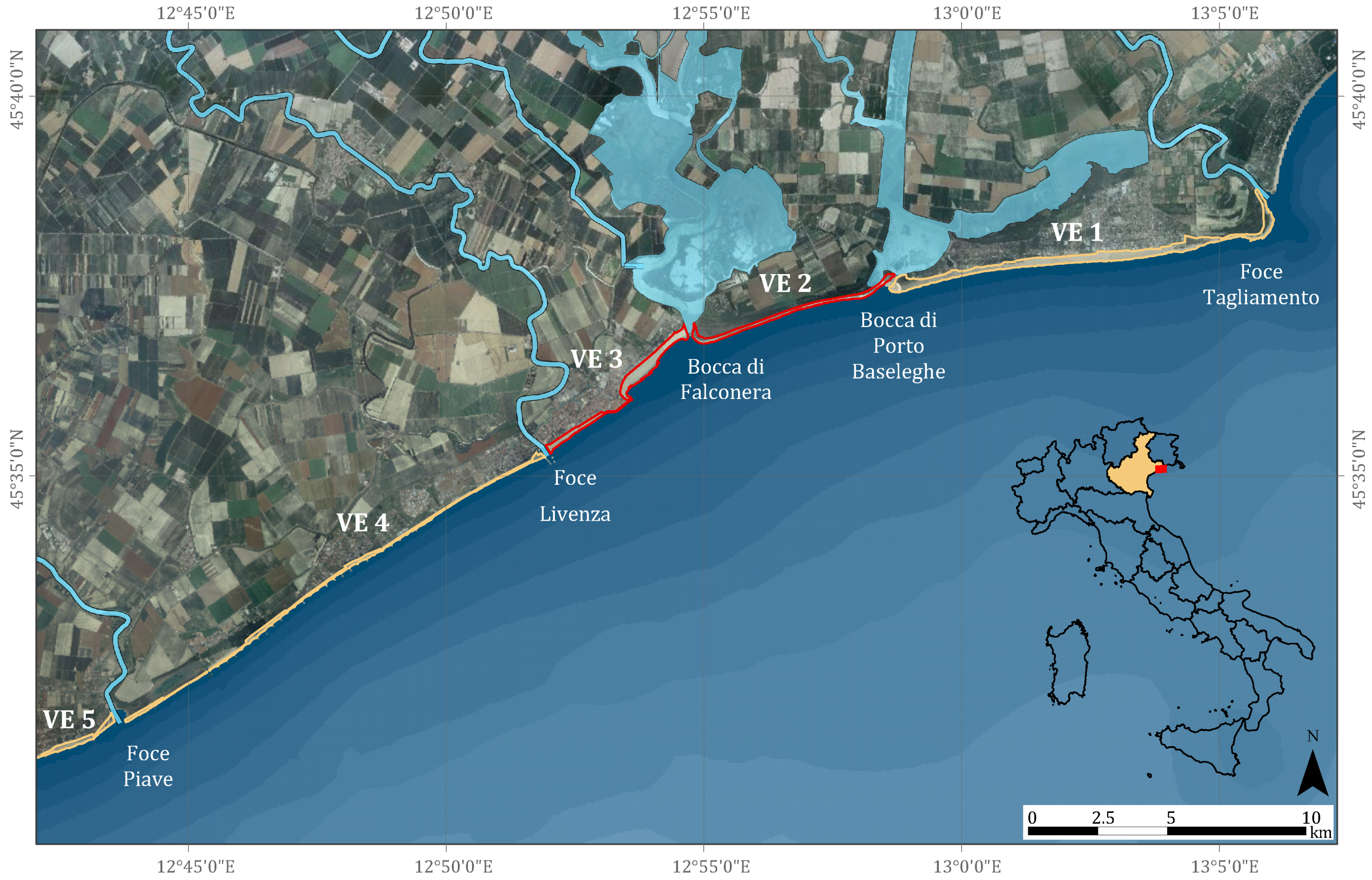
3. An Application to Two Stretches of the Venetian Littoral

The aim of this section is to present local inundation maps produced for two stretches of the Venetian littoral (Figure 5), which show the annual probability of exceedance for a given flood level. A detailed description of this littoral is given in [48] where, for a better understanding of sediment transport patterns, the coast of the Veneto region is subdivided into 20 homogeneous littoral cells separated by lagoon inlets or river mouths.
The Adriatic coast is plagued by a combination of high waves and storm surges, which are responsible for the flooding of coastal areas, in particular, Venice and its lagoon. The north Adriatic Sea is characterized by two main wind (and correspondingly wave) regimes, which are primarily influenced by local orography. The prevailing winds along the Venetian coastline are the Bora and the Scirocco, which blow from the northeast and southeast, respectively. In [49], information and data for the Venetian littoral are collected, harmonized and stored in a single geographical information system (called Coastal GIS).
This information comprises topographic and bathymetric surveys over a range of time (bathymetry: 2005, 2007/2008, 2010, and 2012/2014; DTM and DEM: 2008and 2012/2013) that are essential for both the wave transformation model and for the flooding model. The latest available information was used as input in the models. More in detail, DTM representing the inland topography have a grid size equal to 1 m. A common frame for vertical reference data was considered.
A wave dataset measured (1987–2017) at the oceanographic tower “Acqua Alta” situated on 16 m of water depth. (MLLW) in the Gulf of Venice (Lat 45 18’51.27” N, Lon: 12 30’29.93” E) allowed statistically analyzing the marine climate along this coast. Different wave gauges have been used since the start of the measurements at the Acqua Alta research tower and the instrument system has been progressively upgraded and repositioned during maintenance operations. The registered data include: significant wave height H s (m), maximum wave height H M A X , mean period T m and peak period T s (s), mean wave direction ( N), and sea level ζ (m ZMPS, where ZMPS is a reference level for Venice named Zero Mareografico Punta della Salute). Figure 6 shows the time series of the recorded significant wave height (black line).
The data sample, selected from the measurements following the aforementioned procedure and selecting H c r i t 1.5 H s M e a n = 1 m and d c r i t = 3 h, includes 974 wave storms recorded from 1987 to 2017 and it was also used to find some correlation among variables. The dots in Figure 6, together with the wave series, represent the maximum significant wave heights of the 974 storms; green dots are the peaks over threshold 1 m, while red dots are the peaks over threshold 2.5 m.
In Figure 7a, the wave heights H s of each storm are plotted against their corresponding wave periods and classified on the basis of their wave steepness ( H s / L 0 ), allowing to evaluate the dependency law between this two variable. Figure 7b shows the duration of the storm d, defined as the time interval in which the significant wave height exceeds the 50% of H s M A X and includes the maximum measured wave height H s M A X of the storm. Moreover, the transformation from the space of physical variables to the standardized variable space was applied to the data sample. The transformation applied (in the following F T ( H s , ζ ) ) was based on the Nataf transformation [50], which describes the joint probability density function of random variables based on their individual marginal distributions and the coefficients of correlation using a Gaussian copula.
Finally, twenty couples of wave heights H S and sea levels ζ were chosen as offshore input, as reported in Figure 8. The twenty resulting maps were considered sufficient to define the failure domain in detail. The wave steepness was chosen equal to 0.04, therefore the wave period T p was estimated as T p = 3.75 H s 0.554 and the typical total storm duration was assumed equal to the typical value of 4 h, with 30 min of ramping up and 30 min of ramping down.
Since maps of the land uses are not available, for all simulations, a uniform friction coefficient was applied K s = 33 m 1 / 3 s 1 .
The following subsections present the results obtained by applying the proposed methodology in two different littoral cells (visible in Figure 5): the Valle Vecchia coastline (littoral cell No. VE2) and the Caorle coastline (littoral cell No. VE3), characterized by very different land uses.

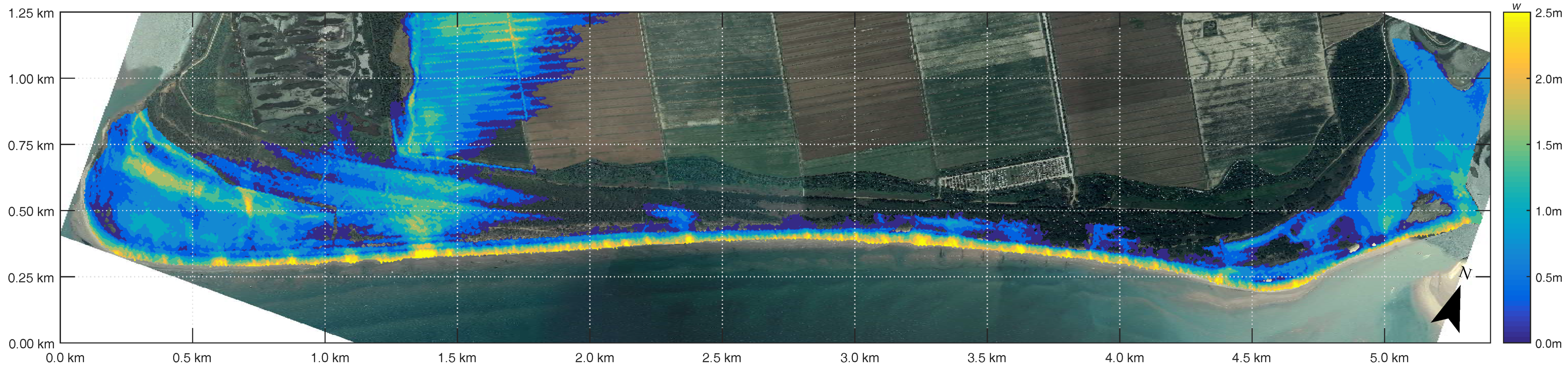
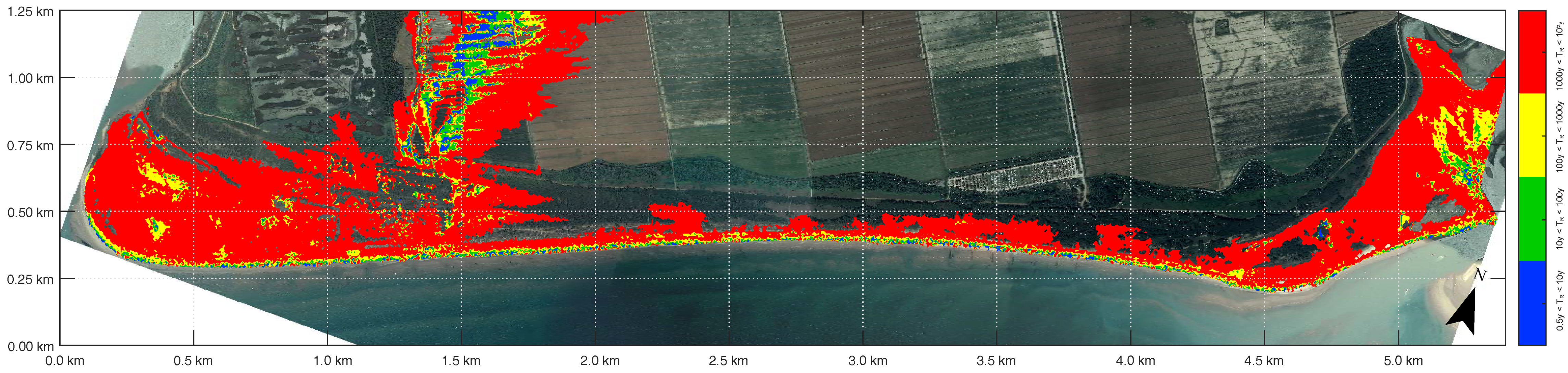
3.1. Valle Vecchia Littoral Cell

The Valle Vecchia coastline (VE2 cell) is 5.5 km long and confined by lagoon’s inlets of Baseleghe at the northeast and Falconera at the southwest. The entire cell is a major environmental area, protected and designated as Natura 2000 sites (SCI IT3250033 and SPA IT3250041), free of urban and tourist settlements and without any coastal defence structure. In the back-shore, a system of dunes is present. Behind the dunes, there are valleys and crop fields. The long-shore sediment transport, coming from the northern cell (VE1) is equal to ∼50,000 m 3 /year. Analyzing the recent evolution of the shoreline, it is possible to verify that the cell is substantially in accretion, even if dunes are subject to local erosion. In fact, the risk of coastal flooding is high and sometimes inundation occurred in the back-shore valley. The water has always entered through some gaps (mainly for pedestrian or vehicle paths) on the dunes. The topographic data highlight different dunes, with crest height in the range 2–5 m.
The aforementioned steps for the coastal flooding risk assessment were applied to the Valle Vecchia coastline. Figure 9 shows an example of flooding maps for H s = 6 m and ζ = 1.75 m ZMPS: some areas are inundated, mainly close to the lagoon’s inlet of Falconera.
From the 20 maps created, it is possible to extract, for every pixel, which couples of H s and ζ caused a level of inundation equal to 50 cm (limit state). The transformation F T ( H s , ζ ) , previously defined, was applied to every couple and, following the FORM methods, the probability of failure p f was evaluated in the whole littoral cell. Figure 10 shows this result, i.e., the present hazard map arranged with a chosen limit state equal to 0.5 m. The area characterized by a return period lower than 10 years is ∼0.1 km 2 .
Figure 11a shows a zoom of the hazard map and highlights that a portion of the valleys and crop fields located behind the dunes have a T R < 10 years. Therefore, the probability that these parts are inundated is very high.

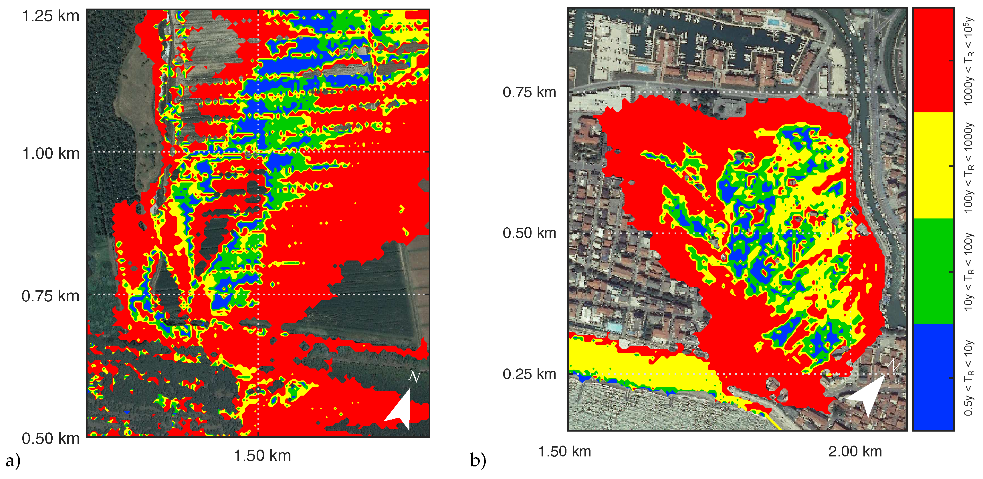
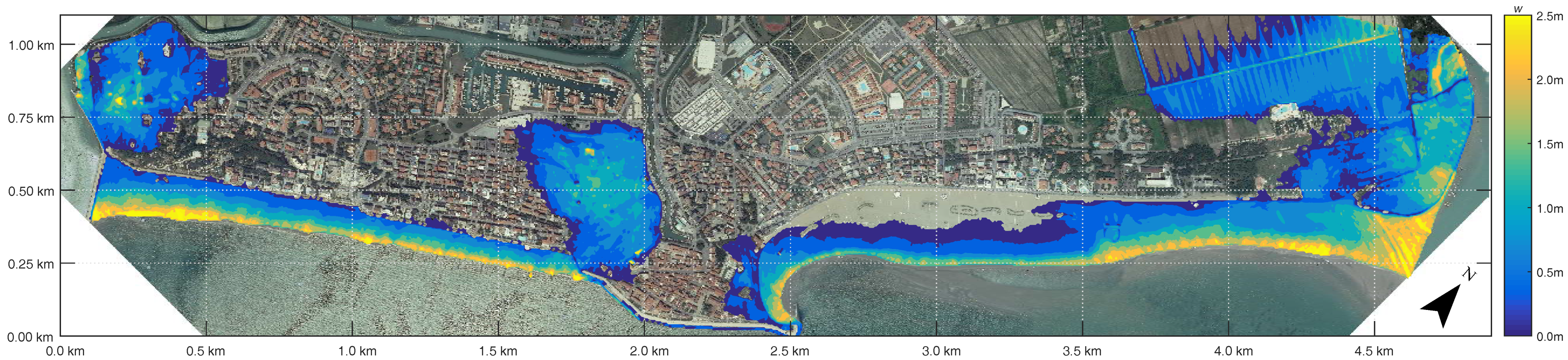
3.2. Caorle Littoral Cell

The Caorle coastline (VE3 cell in Figure 5) is 5 km long, its borders are the mouth of the lagoon’s channel Falconera to the north and the mouth of the River Livenza to the south, both armored with jetties. The economy is mainly based on tourism (∼4,500,000 visitors in 2017) and fishing.
The cell can be subdivided into three main parts: (i) “Spiaggia di Levante” at northeast; (ii) “Murazzi” in the central part; and (iii) “Spiaggia di Ponente” at southwest. The first stretch of this coast at northeast (named “Spiaggia di Levante”) has a normal shoreline direction equal to 140 N, very different from the adjacent ones. This coast is characterized by very fine sediments, with silty fraction that causes drainage problems and occasionally, during the most intense precipitation, the formation of puddles. The emerged beach is very wide and the submerged beach is characterized by gentle slopes. The long-shore sediment transport is ∼20,000 m 3 /year, directed from northeast to southwest.
The historic centre of Caorle is located in the central part. This stretch of coast (800 m long) is bordered at north by a cusp, where a church named “Chiesa della Madonna dell’Angelo” is located. To mitigate the risk to human health, economic activities and cultural heritage, the shoreline position in the central area is stabilized by a sea wall (named “Murazzi”).
In the southern part, the long-shore sediment transport remains approximately equal to 20,000 m 3 /year, again directed from northeast to the southwest. This sand partly nourishes the beach named “Spiaggia di Ponente”, partly deposits in the area next to the jetty of the mouth of the River Livenza and only a few thousand cubic meters go to the southern cell (VE4). Some portions of the town have ground elevations lower than 0.5 m and no system of dunes is present.
The aforementioned steps for the coastal flooding hazard assessment were applied to the Caorle coastline. Figure 12 shows the flooding maps for H s = 6 m, ζ = 1.5 m ZMPS: the historic town is partly flooded and the overtopping occurs at the southern bound of the seawall.
As for the previous stretch of coast, following the FORM methods, present hazard map was arranged with a chosen limit state equal to 0.5 m (Figure 13). The town centre, as expected, has some portions with a high probability of failure ( T R < 10 years). Moreover, the zones next to the two mouths (Falconera and Livenza) are partially exposed to coastal flooding hazard. More in general, the area characterized by a return period lower than 10 years is only ∼70,000 m 2 .
Figure 13. Hazard map (cell VE3): Probability that flooding level 0.5 m is exceeded, expressed as return period T R .
Water 11 00134 g013
Figure 11b shows a zoom of the hazard map and highlights that a portion of the historic city have a T R < 10 years.

4. Discussion

The obtained maps suffer from a number of limitations and simplifications of the hydrodynamic model used. However, the proposed probabilistic methodology has a wider perspective, since it allows drawing maps of coastal flooding vulnerability on the basis of a general flood inundation model.
The methodology can be easily coupled with other models to include other key aspects of the coastal flooding assessment. For example, the boundary conditions can be linked with meteorological models to include the effects of hurricanes, typhoons and cyclones and/or with riverine models. In fact, the combinations of multiple phenomena, not only related to sea conditions, frequently exacerbate the effect of marine inundation. For instance, the simultaneous occurrence of intense precipitations or river overflows (in areas such as deltas and estuaries) with extreme waves and sea levels could contribute to coastal flooding. Similarly, the presence of a drainage system could be less efficient than expected during sea storms, generating critical scenarios.
A single failure mechanism is taken into account in this study, i.e., the overtopping. This mechanism is suited to represent coastal flooding in areas with “rigid boundaries”, for example an area with concrete sea walls or with paved coastal roads that typically are not subject to local damage or collapse. In other cases, however, other features, can influence failure in the long term, for instance, local erosion and, more generally, morphological changes in the topography (for example, the breaching of a dune system or of a fragile coastal defence structure). The inclusion of this mechanism is not straightforward since it involves a deep knowledge of sea–dike/dune resistance and, in the long term, its maintenance strategy (e.g., nourishment and dunes reinforcement).

5. Conclusions

This paper presents a numerical model for the inland flood propagation and an approach for the assessment of coastal flooding vulnerability. The proposal is a novel 2D model that solves the shallow-water equations using a linearized friction term and assumes negligible advective accelerations. The formulation takes advantage of an appropriate vectorization method and a positivity preserving scheme. The key feature of this model is the fast computational speed obtained by means of a formulation suited to GPU cards, thus making it ideal for handling high-resolution maps on a regional scale.
An application to the Venetian coast was carried out, thanks to a wide geomorphological and hydraulic knowledge of this regional area. The statistical analysis of the main marine drivers acting on this coast was carried out to force the wave transformation model and to obtain the boundary condition to be imposed to the shoreline. Finally, a Level II reliability analysis was applied to the results gained through the flooding propagation model, establishing the desired hazard maps. Two hazard maps were produced, showing the probability that any point/pixel is flooded by at least 50 cm.
The methodology seems promising and meets the requirements of local stakeholders for a flexible tool that predicts coastal flooding and highlights the more exposed and vulnerable areas, as the hardware required (GPU) to run the model is certainly well within the financial and technical means of local administrations, unlike the large cluster of CPUs needed to run the existing operational dynamic models.
Finally, the produced hazard maps could be easily integrated with information on the exposed values in the coastal area (e.g., indicative number of inhabitants potentially affected, type of economic activity of the area potentially affected, and installation which might cause accidental pollution in case of flooding [51]) to prepare flood risk maps that show the potential adverse consequences for human health, the environment, cultural heritage and economic activity associated with coastal flooding.

Author Contributions

Conceptualization and Methodology, C.F., L.M. and P.R.; Investigation, C.F., L.M. and P.R.; Writing—Review and Editing, C.F., L.M. and P.R.; Supervision, C.F., L.M. and P.R.

Funding

The Agreement between Regione Veneto and University of Padova entitled “Gestione Integrata della Zona Costiera. Progetto per lo studio ed il monitoraggio della linea di costa per la definizione degli interventi di difesa dei litorali dall’erosione nella Regione Veneto” is gratefully acknowledged.

Conflicts of Interest

The authors declare no conflict of interest.

References

  1. Cazenave, A.; Cozannet, G.L. Sea level rise and its coastal impacts. Earth’s Future 2014, 2, 15–34. [Google Scholar] [CrossRef] [Green Version]
  2. Pomaro, A.; Cavaleri, L.; Lionello, P. Climatology and trends of the Adriatic Sea wind waves: Analysis of a 37-year long instrumental data set. Int. J. Climatol. 2017, 37, 4237–4250. [Google Scholar] [CrossRef]
  3. Rahmstorf, S. Rising hazard of storm-surge flooding. Proc. Natl. Acad. Sci. USA 2017, 114, 11806–11808. [Google Scholar] [CrossRef] [PubMed] [Green Version]
  4. Nicholls, R.J.; Cazenave, A. Sea-level rise and its impact on coastal zones. Science 2010, 328, 1517–1520. [Google Scholar] [CrossRef] [PubMed]
  5. Vafeidis, A.T.; Nicholls, R.J.; McFadden, L.; Tol, R.S.; Hinkel, J.; Spencer, T.; Grashoff, P.S.; Boot, G.; Klein, R.J. A new global coastal database for impact and vulnerability analysis to sea-level rise. J. Coast. Res. 2008, 24, 917–924. [Google Scholar] [CrossRef]
  6. Zanuttigh, B.; Simcic, D.; Bagli, S.; Bozzeda, F.; Pietrantoni, L.; Zagonari, F.; Hoggart, S.; Nicholls, R.J. THESEUS decision support system for coastal risk management. Coast. Eng. 2014, 87, 218–239. [Google Scholar] [CrossRef]
  7. Zachry, B.C.; Booth, W.J.; Rhome, J.R.; Sharon, T.M. A national view of storm surge risk and inundation. Weather Clim. Soc. 2015, 7, 109–117. [Google Scholar] [CrossRef]
  8. Wadey, M.P.; Nicholls, R.J.; Hutton, C. Coastal flooding in the Solent: An integrated analysis of defences and inundation. Water 2012, 4, 430–459. [Google Scholar] [CrossRef]
  9. Spaulding, M.L.; Grilli, A.; Damon, C.; Fugate, G.; Oakley, B.A.; Isaji, T.; Schambach, L. Application of state of art modeling techniques to predict flooding and waves for an exposed coastal area. J. Mar. Sci. Eng. 2017, 5, 10. [Google Scholar] [CrossRef]
  10. Aucelli, P.P.C.; Di Paola, G.; Incontri, P.; Rizzo, A.; Vilardo, G.; Benassai, G.; Buonocore, B.; Pappone, G. Coastal inundation risk assessment due to subsidence and sea level rise in a Mediterranean alluvial plain (Volturno coastal plain–southern Italy). Estuarine Coast. Shelf Sci. 2017, 198, 597–609. [Google Scholar] [CrossRef]
  11. Di Luccio, D.; Benassai, G.; Di Paola, G.; Rosskopf, C.; Mucerino, L.; Montella, R.; Contestabile, P. Monitoring and modelling coastal vulnerability and mitigation proposal for an archaeological site (Kaulonia, Southern Italy). Sustainability (Switzerland) 2018, 10, 2017. [Google Scholar] [CrossRef]
  12. Di Risio, M.; Bruschi, A.; Lisi, I.; Pesarino, V.; Pasquali, D. Comparative Analysis of Coastal Flooding Vulnerability and Hazard Assessment at National Scale. J. Mar. Sci. Eng. 2017, 5, 51. [Google Scholar] [CrossRef]
  13. Gallien, T. Validated coastal flood modeling at Imperial Beach, California: Comparing total water level, empirical and numerical overtopping methodologies. Coast. Eng. 2016, 111, 95–104. [Google Scholar] [CrossRef]
  14. Lerma, A.; Bulteau, T.; Elineau, S.; Paris, F.; Durand, P.; Anselme, B.; Pedreros, R. High-resolution marine flood modelling coupling overflow and overtopping processes: Framing the hazard based on historical and statistical approaches. Nat. Hazards Earth Syst. Sci. 2018, 18, 207–229. [Google Scholar] [CrossRef]
  15. Simeoni, U.; Corbau, C. A review of the Delta Po evolution (Italy) related to climatic changes and human impacts. Geomorphology 2009, 107, 64–71. [Google Scholar] [CrossRef]
  16. Carbognin, L.; Teatini, P.; Tosi, L. Eustacy and land subsidence in the Venice Lagoon at the beginning of the new millennium. J. Mar. Syst. 2004, 51, 345–353. [Google Scholar] [CrossRef]
  17. Martinelli, L.; Zanuttigh, B.; Corbau, C. Assessment of coastal flooding hazard along the Emilia Romagna littoral, IT. Coast. Eng. 2010, 57, 1042–1058. [Google Scholar] [CrossRef]
  18. Pescaroli, G.; Magni, M. Flood warnings in coastal areas: How do experience and information influence responses to alert services? Nat. Hazards Earth Syst. Sci. 2015, 15, 703–714. [Google Scholar] [CrossRef]
  19. Wolshon, B.; Urbina, E.; Wilmot, C.; Levitan, M. Review of policies and practices for hurricane evacuation. I: Transportation planning, preparedness, and response. Nat. Hazards Rev. 2005, 6, 129–142. [Google Scholar] [CrossRef]
  20. Jia, X.; Morel, G.; Martell-Flore, H.; Hissel, F.; Batoz, J.L. Fuzzy logic based decision support for mass evacuations of cities prone to coastal or river floods. Environ. Model. Softw. 2016, 85, 1–10. [Google Scholar] [CrossRef]
  21. Kunreuther, H.; Pauly, M. Rules rather than discretion: Lessons from Hurricane Katrina. J. Risk Uncertain. 2006, 33, 101–116. [Google Scholar] [CrossRef]
  22. Burcharth, H.F.; Zanuttigh, B.; Andersen, T.L.; Lara, J.L.; Steendam, G.J.; Ruol, P.; Sergent, P.; Ostrowski, R.; Silva, R.; Martinelli, L.; et al. Chapter 3—Innovative Engineering Solutions and Best Practices to Mitigate Coastal Risk. In Coastal Risk Management in a Changing Climate; Butterworth-Heinemann: Boston, MA, USA, 2015; pp. 55–170. [Google Scholar]
  23. Vanderlinden, J.P.; Baztan, J.; Coates, T.; Dávila, O.G.; Hissel, F.; Kane, I.O.; Koundouri, P.; McFadden, L.; Parker, D.; Penning-Rowsell, E.; et al. Chapter 5—Nonstructural Approaches to Coastal Risk Mitigations. In Coastal Risk Management in a Changing Climate; Butterworth-Heinemann: Boston, MA, USA, 2015; pp. 237–274. [Google Scholar]
  24. Kusumo, A.; Reckien, D.; Verplanke, J. Utilising volunteered geographic information to assess resident’s flood evacuation shelters. case study: Jakarta. Appl. Geogr. 2017, 88, 174–185. [Google Scholar] [CrossRef]
  25. Coastal Flooding Hazard—Community information and participation. Available online: https://coastalfloodinghazard.wordpress.com/community-information (accessed on 7 January 2019).
  26. Hoggart, S.; Hawkins, S.J.; Bohn, K.; Airoldi, L.; van Belzen, J.; Bichot, A.; Bilton, D.T.; Bouma, T.J.; Colangelo, M.A.; Davies, A.J.; et al. Chapter 4–Ecological Approaches to Coastal Risk Mitigation. In Coastal Risk Management in a Changing Climate; Butterworth-Heinemann: Boston, MA, USA, 2015; pp. 171–236. [Google Scholar]
  27. Gómez-Pina, G.; Muñoz-Pérez, J.J.; Ramírez, J.L.; Ley, C. Sand dune management problems and techniques, Spain. J. Coast. Res. 2002, 36, 325–332. [Google Scholar] [CrossRef]
  28. Favaretto, C.; Martinelli, L.; Ruol, P. A Model of Coastal Flooding Using Linearized Bottom Friction and its Application to a Case Study in Caorle, Venice Italy. Int. J. Off. Polar Eng. 2019, 29, 1–9. [Google Scholar]
  29. Favaretto, C.; Martinelli, L.; Ruol, P. Raster Based Model of Inland Coastal Flooding Propagation Using Linearized Bottom Friction and Application to a Real Case Study in Caorle, Venice (IT). In Proceedings of the 28th International Ocean and Polar Engineering Conference, Sapporo, Japan, 10–15 June 2018. [Google Scholar]
  30. Bates, P.D.; Horritt, M.S.; Fewtrell, T.J. A simple inertial formulation of the shallow water equations for efficient two-dimensional flood inundation modelling. J. Hydrol. 2010, 387, 33–45. [Google Scholar] [CrossRef]
  31. Hunter, N.M.; Bates, P.D.; Horritt, M.S.; Wilson, M.D. Simple spatially-distributed models for predicting flood inundation: A review. Geomorphology 2007, 90, 208–225. [Google Scholar] [CrossRef]
  32. Khorshid, S.; Mohammadian, A.; Nistor, I. Extension of a well-balanced central upwind scheme for variable density shallow water flow equations on triangular grids. Comput. Fluids 2017, 156, 441–448. [Google Scholar] [CrossRef]
  33. Brodtkorb, A.R.; Sætra, M.L.; Altinakar, M. Efficient shallow water simulations on GPUs: Implementation, visualization, verification, and validation. Comput. Fluids 2012, 55, 1–12. [Google Scholar] [CrossRef]
  34. Liang, W.Y.; Hsieh, T.J.; Satria, M.T.; Chang, Y.L.; Fang, J.P.; Chen, C.C.; Han, C.C. A GPU-based simulation of tsunami propagation and inundation. In Proceedings of the International Conference on Algorithms and Architectures for Parallel Processing; Springer: Berlin/Heidelberg, Germany, 2009; pp. 593–603. [Google Scholar]
  35. Synolakis, C. The runup of solitary waves. J. Fluid Mech. 1987, 185, 523–545. [Google Scholar] [CrossRef]
  36. Briggs, M.J.; Synolakis, C.E.; Harkins, G.S.; Green, D.R. Laboratory experiments of tsunami runup on a circular island. Pure Appl. Geophys. 1995, 144, 569–593. [Google Scholar] [CrossRef]
  37. Kottegoda, N.; Rosso, R. Probability, Statistics, and Reliability for Civil and Environmental Engineers; McGraw-Hill: New York, NY, USA, 1997. [Google Scholar]
  38. Madsen, H.O.; Krenk, S.; Lind, N.C. Methods of Structural Safety; Courier Corporation: North Chelmsford, MA, USA, 2006. [Google Scholar]
  39. Du, X. First order and second reliability methods. In Probabilistic Engineering Design; John Wiley & Sons Inc.: Hoboken, NJ, USA, 2005; pp. 1–33. [Google Scholar]
  40. Hasofer, A.M.; Lind, N.C. Exact and invariant second-moment code format. J. Eng. Mech. Div. 1974, 100, 111–121. [Google Scholar]
  41. Group, T.W. The WAM model—A third generation ocean wave prediction model. J. Phys. Oceanogr. 1988, 18, 1775–1810. [Google Scholar] [CrossRef]
  42. Armaroli, C.; Ciavola, P.; Perini, L.; Calabrese, L.; Lorito, S.; Valentini, A.; Masina, M. Critical storm thresholds for significant morphological changes and damage along the Emilia-Romagna coastline, Italy. Geomorphology 2012, 143, 34–51. [Google Scholar] [CrossRef]
  43. Boccotti, P. On coastal and offshore structure risk analysis. Excerpta Ital. Contrib. Field Hydraul. Eng. 1986, 1, 19–36. [Google Scholar]
  44. Mendoza, E.; Jimenez, J.; Mateo, J.; Salat, J. A coastal storms intensity scale for the Catalan sea (NW Mediterranean). Nat. Hazards Earth Syst. Sci. 2011, 11, 2453–2462. [Google Scholar] [CrossRef] [Green Version]
  45. Archetti, R.; Paci, A.; Carniel, S.; Bonaldo, D. Optimal index related to the shoreline dynamics during a storm: The case of Jesolo beach. Nat. Hazards Earth Syst. Sci. 2016, 16, 1107–1122. [Google Scholar] [CrossRef]
  46. Lin-Ye, J.; García-León, M.; Gràcia, V.; Ortego, M.I.; Stanica, A.; Sánchez-Arcilla, A. Multivariate hybrid modelling of future wave-storms at the northwestern Black Sea. Water 2018, 10, 221. [Google Scholar] [CrossRef]
  47. Dally, W.R.; Dean, R.G.; Dalrymple, R.A. Wave height variation across beaches of arbitrary profile. J. Geophys. Res. Oceans 1985, 90, 11917–11927. [Google Scholar] [CrossRef]
  48. Ruol, P.; Martinelli, L.; Favaretto, C. Vulnerability Analysis of the Venetian Littoral and Adopted Mitigation Strategy. Water 2018, 10, 984. [Google Scholar] [CrossRef]
  49. Ruol, P.; Martinelli, L.; Favaretto, C. Gestione Integrata Della Zona Costiera. Studio e Monitoraggio per la Definizione Degli Interventi di Difesa dei Litorali Dall’Erosione Nella Regione Veneto—Linee Guida; Edizioni Libreria Progetto; University of Padua: Padova, Italy, 2016. [Google Scholar]
  50. Nataf, A. Determination des Distribution don’t les marges sont Donnees. C. R. Acad. Sci. 1962, 225, 42–43. [Google Scholar]
  51. Prinos, P.; Kortenhaus, A.; Swerpel, B.; Jiménez, J.A. Review of Flood Hazard Mapping; Floodsite Report, No. T03-07-01,54; University of Athens: Athens, Greece, 2008. [Google Scholar]
Figure 1. (a) Joint probability density function in X-plane and performance function g ( X 1 , X 2 ) = 0 ; and (b) joint pdf in U-plane and performance function g ( U 1 , U 2 ) = 0 .
Water 11 00134 g001
Figure 2. Example of the wave transformation model results and definition of the boundary conditions at the isobath 0 m.
Water 11 00134 g002
Figure 3. Example of final boundary condition at the shoreline refereed to the Mean Sea Level (MSL).
Water 11 00134 g003
Figure 4. (a) Example of evaluation of the limit state in the physical space; and (b) limit state in standard space g(U) and evaluation of the distance β .
Water 11 00134 g004
Figure 5. The northern part of the Venetian littoral and its subdivision into coastal cells: VE1, Bibione; VE2, Valle Vecchia; VE3, Caorle; VE4, Porto Santa Margherita–Duna Verde–Eraclea; VE5, Jesolo.
Water 11 00134 g005
Figure 6. Time series of significant wave height H s (black line), where dots represent the 974 storms: green dots are peak over threshold 1 m, while red dots are peak over threshold 2.5 m.
Water 11 00134 g006
Figure 7. (a) H s , T p and steepness H s / L correlation; and (b) storm duration d vs. H s .
Water 11 00134 g007
Figure 8. Red dots are the couple H s ζ chosen as input for the models (ZMPS is a reference level for Venice).
Water 11 00134 g008
Figure 9. Flooding map (cell VE2): H s = 6 m, ζ = 1.75 m ZMPS.
Water 11 00134 g009
Figure 10. Hazard map (cell VE2): Probability that flooding level 0.5 m is exceeded, expressed as return period T R .
Water 11 00134 g010
Figure 11. (a) Zoom of the Valle Vecchia hazard map shown in Figure 10; and (b) zoom of the Caorle hazard map shown in Figure 13.
Water 11 00134 g011
Figure 12. Flooding map (cell VE3): H s = 6 m, ζ = 1.5 m ZMPS.
Water 11 00134 g012

