Article

Laboratory Investigation on the Evolution of a Sandy Beach Nourishment Protected by a Mixed Soft–Hard System

1
Department of Civil, Environmental, Building Engineering and Chemistry (DICATECh), Politecnico di Bari, Bari 70126, Italy
2
Department of Civil, Construction-Architectural and Environmental Engineering (DICEAA)—Environmental and Maritime Hydraulic Laboratory (LIam), University of L’Aquila, L’Aquila 67100, Italy
*
Author to whom correspondence should be addressed.
These authors contributed equally to this work.
Water 2018, 10(9), 1171; https://doi.org/10.3390/w10091171
Submission received: 30 July 2018 / Revised: 21 August 2018 / Accepted: 27 August 2018 / Published: 31 August 2018

Abstract

:
A new experimental campaign on a 2D movable-bed physical model, reproducing a typical nourishment sandy beach profile, is being carried out in the wave flume of the Laboratory of Coastal Engineering at Politecnico di Bari (Bari, Italy). The main aim is to assess the short-term evolution of a sandy beach nourishment, relying on a mixed solution built on the deployment of a Beach Drainage System (BDS) and a rubble-mound detached submerged breakwater. This paper aims at illustrating the experimental findings. Tests presented herein deal with both unprotected and protected configurations, focusing on the hydrodynamic and morphodynamic processes under erosive conditions. Results show that, with respect to the unprotected conditions, BDS reduces the shoreline retreat and the beach steepen within swash and surf zone as well. Moreover, a reduction of net sediment transport rate is observed. When BDS is coupled with the submerged sill, a reversal of the prevalent direction of the net sediment transport seaward occurs offshore the sheltered region. Less considerable positive effects on shoreline retreat are induced by the submerged structure, whereas the mean beach slope remains quite stable. Secondary effects of drain on the submerged sill performance are also highlighted. BDS reduces wave-induced setup on beach, by mitigating the mean water level raising, typically experienced by such structures.

1. Introduction

Coasts are naturally affected by erosion processes enhanced by climate changes, raising urbanisation and exploitation of coastal zones. Beach size is decreasing with unfavourable consequences for the environment, society and economy. Coastal defence and mitigation interventions appear to be essential and the timing for decisions dealing with coastal protection against climate change should be taken at the early stage [1,2,3]. In such a context, it was observed that upgrading coastal defences and nourishing beaches would reduce the impacts related to climate change roughly by three orders of magnitude [4].
Several methods, ranging from standard rubble mound breakwaters (e.g., [5,6]) up to low-environmental impact solutions (e.g., beach nourishments, artificial reefs and by-pass systems (e.g., [7,8,9,10])), are typically deployed to recover and protect beaches from erosion. However, effects of defence work are not always sustainable under both environmental and economical points of view. Hard structures often cause a shift of erosion process along neighbouring areas, whereas soft solutions demonstrate to be long-term unsustainable. Among the latter, beach nourishments constitute the most used method. They can be considered as examples of environment-friendly solution for beach restoration and coastal preservation, basically consisting of filling the near-shore region with new sediment to restore or maintain an adequate beach width and ensure an appropriate dune protection, without compromising coastal environment and tourism.
To limit sediment losses during intervention lifetime, nourishment works are frequently combined with hard coastal defence structures, since they reduce sediment spreading and lengthen the time span between periodic re-nourishments for coastal restoration. On the other hand, defence structures influence wave propagation and reduce the environmental sustainability of the intervention. To reduce such impacts on environment, submerged breakwaters are widely used as shore protection system aimed at preventing shoreline retreat. They dissipate the incident wave energy, hence reducing the wave hydrodynamic action on coasts [11,12] and extending the residence time of sediments in the sheltered region [13,14], depending on configuration parameters (i.e., freeboard, distance from the shoreline, and transmission coefficient), wave climate and nearshore seabed [15,16,17,18]. Moreover, they have a lower impact on both hydrodynamic processes and nearshore zone morphodynamics with respect to the emerged detached breakwaters and groins, since they are able to enhance the water circulation, its renovations rates [19,20] and biological biodiversity [21].
Past studies show that sandy beach stability could also be increased by the deployment of a Beach Drainage System (BDS), which is counted among soft-engineering systems aimed at contrasting erosion. Previous works [22,23,24] demonstrate the importance of the close link between the swash zone sediment transport and groundwater. In particular, they demonstrate that a lower position of groundwater with respect to mean sea level can affect morphodynamics, by inducing a sediment stabilisation when infiltration inside the beach occurs. The BDS is able to increase the apparent sand permeability, by inducing within the beach an artificial lowering of the saturation line and an increase in the thickness of the unsaturated area. In this way, up-rush flux is more easily absorbed by the beach, whereas sea-ward flow is significantly reduced.
Currently, drainage efficacy in restoring eroded beaches is not well defined. BDS can be considered as an auxiliary system in coasts management, such as combined with a beach nourishment to increase sediment stability and, hence, the nourishment lifetime [25]. Field installations deployed around the world (e.g., Denmark, USA, UK, Japan, Spain, Sweden, Holland, France, Italy, and Malaysia) were not supported by an adequate long-term monitoring to highlight a full scientific evidence of beach stabilisation, mainly due to both the erroneous management and the non-existent maintenance of the systems. However, in some cases, an overall reasonable performance in short-medium term (1–5 years), was reported [26]. Moreover, even though the BDS concept was initiated about fifty years ago and many BDSs have been installed worldwide since 1981 [27], the first experimental studies on BDS morphodynamic and hydrodynamic performances were carried recently [28,29]. In 2010, full-scale laboratory experiments were carried out to overcome the limitations of previous studies [30,31,32,33]. The already tested BDS configurations were shown to stabilise the beach for medium and low energy conditions, while for high energy wave attacks the drainage system seemed to be inadequate in giving any stabilisation effect [34,35].
Another important issue related to beach nourishment design is related to the retrieval of nourished sediments with specific characteristics, fully compatible with the existing grain size and composition (i.e., mineralogy). Both the choice of sediments and the sampling area influence not only the further evolution of coastline and the beach response [36], but also the impact on environment. In general, the material necessary for nourishments comes from dredging operations (of navigation channels, harbour entrances or basins) or from mining sites (land or submarine). In all cases, the compatibility between added and native sediments is fundamental to assess the suitability of mining sites and the sediment volumes required to ensure nourishment stability, manage subsequent periodic recharging operations and prevent the intervention area, which could suffer dramatic consequences due to high turbidity during the works [37,38,39].
Due to both the high costs of sediment recovery and dredging operations and the significant time required for large nourishment projects, beach scraping may represent an attractive option [40,41,42], being widely undertaken and often privately supported by beach managers. Such a kind of small periodical interventions could constitute a valid alternative with respect to traditional large nourishment projects for recovering beaches [43], since small sediment volumes are required, with consequent reduced costs, working time and minimal impacts on coastal natural cycles. The sediment could be easily mined from the active littoral zone, ensuring the compatibility of the sediment source [44].
Beach nourishments, as well as beach scraping, can indeed be recognised as able to counteract beach erosion and, hence, limit the effects of climate changes on coastal flood risk due to beach erosion [45]. Of course, the approach should be environmentally sustainable.
Our research aims at investigating a mixed approach, relying on both standard and innovative beach defence systems, by gaining insight on the cross-shore, short term morphodynamic response of a beach nourishment protected by a rubble-mound detached submerged breakwater and a BDS deployed together. Unique and definitive design guidelines on BDS are still missing, since previous field installation did not provide an adequate long-term monitoring and laboratory experiments were mainly focused on the study of the hydrodynamics, by neglecting the role of longshore gradients in the morphodynamics evolution. The novelty of our research lies in assessing the reliability of the mixed approach in beach stabilisation. The basic idea is to switch high energy sea states propagating from offshore to medium/low energy waves in the surf zone, by means of the submerged breakwater, to enhance the efficiency of BDS and improve sandy nourishment performance by increasing the intervention lifetime, without affecting its low-environmental impact.
A modelling campaign on a 2D physical small scale model of a typical nourished sandy beach profile is being carried out. The tests presented herein dealt with the investigation of the profile evolution forced by erosive waves, by focusing on its morphological development up to equilibrium and its hydrodynamics. The configurations comprised the unprotected beach, BDS protected and the coupled BDS-breakwater beach cases. Protection systems efficiency is here reported in terms of cross-shore profile evolution, shoreline displacement, submerged bar migration and sediment transport rate. Furthermore, wave parameters and groundwater behaviour inside the beach in the different tested configurations are reported and discussed.

2. Materials and Methods

2.1. Experimental Setup

The experimental tests were performed in the wave flume at the Laboratory of Coastal Engineering of the Department of Civil, Environmental, Building Engineering and Chemistry of the Politecnico di Bari (Bari, Italy). The 2D wave flume used for the experiments is about 50 m long, 2.5 m wide and 1.2 m deep. It is equipped with a piston-type wave maker provided by Wallingford (UK) able to generate regular and irregular wave trains and extreme wave heights of 0.3 m with a maximum water level of 0.8 m. The nourishment profile was reproduced inside the flume as a 2D physical bed movable model. It may be viewed as a Froude scaled typical intervention with a prototype-to-model ratio equal to 1:10. However, as the results are intended to be general, model dimensions are illustrated and discussed as well hereinafter.
In Figure 1, a sketch of the model geometry adopted for the experiments is shown. The initial sandy profile began about 20 m from the wave paddle with a mean slope of 1 / 30 for 9 m, followed by a 1 / 8 sloped foreshore for 5.2 m and a horizontal emerged berm 2.5 m long, + 0.15 m above the mean water level. The total sand volume was of about 18 m 3 .
The adoption of a unique coordinate system was appropriate to analyse measurements derived from different instruments. The x-axis was aligned with the cross-shore direction, pointing to the wave paddle with the origin ( x = 0 ) set at the onshore limit of the sandy beach profile at the flume centreline. The z direction was aligned with the vertical direction, pointing upward with z = 0 at the mean water level. The y-axis was aligned with the long-shore direction.
Sand grain size curve was obtained at LIC, according to A.S.T.M. standard [46], whereas both permeability and water content were measured on reconstituted sand samples at the Geotechnical Engineering Laboratory of Politecnico di Bari. According to Wentworth grain size classes [47], the sand used was an almost uniform medium-fine sand with a D 50 equal to 0.227 mm and D 10 and D 90 equal to 0.177 mm and 0.322 mm, respectively. The sand was characterised by a permeability of 4.1 × 10 5 m/s and a mean water content of about 27 % .
The drainage system was constituted of a drain pipe placed inside the beach, at 0.165 m below the static groundwater level, parallel to the shoreline, covering the total model width (about 2.5 m). Two drain pipes ( D 1 and D 2 in Figure 1) were installed to preliminarily evaluate the drainage performances at different distances from the initial shoreline ( 1 m and 1.5 m, respectively). Drains were 0.07 m diameter PVC pipes, with rectangular holes uniformly distributed along the side surface, allowing the water drainage. Moreover, to avoid the obstruction of the aforesaid holes by the sand, the pipes were covered by a geotextile membrane. The drains were connected through a blind pipe to a manifold well from which the water was removed by means of a pumping system and then fed back into the water circulation system. The on/off drains switch was made possible by means of two valves installed at the end of each pipe, outside the flume, before the connection with the blind pipes.
The dimensions of the rubble-mound submerged breakwater were chosen to switch high energy sea states propagating from offshore to medium/low within the surf zone, for which drainage seems to show a better efficiency [35]. This was achieved by testing a submerged breakwater characterised by a freeboard higher than conventional submerged defence structures. The breakwater was constructed of one layer of natural stones with a median diameter equal to 5 cm in model scale. The landward side of the structure was 2.4 m from the shoreline with a 0.6 m wide crest and a freeboard equal to 0.18 m below the mean water level. Both landward and seaward slopes were 1:2. Other significant dimensions (i.e., sea/landward water depths) are reported in Figure 1.
A constant JONSWAP wave spectrum with peak enhancement factor 3.3 and characterised by nominal significant wave height H s and peak period T p of 0.2 m and 1.5 s, respectively, was reproduced in the flume. The cross-shore nourishment evolution was investigated in both unprotected and protected conditions to compare the effects of the mixed configuration on both hydrodynamics and morphodynamics, forced by the same wave attack, reproducing erosive conditions. The empirical criteria proposed by [48,49,50,51] were used for the scope.
After testing beach profile evolution in unprotected conditions, each drain was tested without the submerged breakwater. Then, the mixed solution constituted by the coupled system of the drain D 1 and the rubble-mound detached submerged breakwater was tested. Each test was subdivided in steps, in accordance with the bottom measurements time-intervals, chosen to follow the quick bed variations occurring in the early stage. Accordingly, surveys were performed every 15 min in the first hour (Steps 1–4) and every 30 min for the second hour (Steps 5 and 6). Then, the profile was surveyed every hour until the fourth hour of test (Steps 7 and 8), every 2 h until the tenth and every 3 h up to equilibrium. In Table 1, tests are reported as performed in chronological order, with the relative reference name ( T e s t I D ). Moreover, the wave bulk parameters (significant wave height H s , zero-order moment wave height H m o , peak period T p and zero-order moment m 0 ) estimated from the offshore wave gauge ( W G 1 ) for each test are reported as mean values of those calculated for each step. Tests were run until beach equilibrium condition was reached, approximately when variations in profile measurements were almost negligible.

2.2. Measurements

Wave transformations along the flume were investigated by means of seven resistive wave gauges placed in the flume central section ( W G 1 W G 7 in Figure 1) by measuring water surface elevations with an acquisition frequency of 20 Hz. Wave parameters were calculated for each test step at wave gauge locations by means of standard zero-crossing and spectral analyses. The offshore wave gauge placed near the wave paddle ( W G 1 ) and gauges W G 2 W G 3 in the unprotected conditions (Figure 1) were used to check the pseudo-random wave trains generated in the flume, since no active absorption system was deployed. In the protected tests B D S 1 , B D S 2 , B D S 1 - B W (Table 1), wave gauges W G 2 W G 4 were moved and located at the foreshore toe in order to estimate the beach reflection coefficients by separating reflected from incident components by means of the method proposed by [52].
Water surface elevations measured from the gauges W G 4 W G 7 and W G 5 W G 7 in unprotected and protected conditions, respectively, were used to evaluate waves propagation along the nearshore. In particular, during tests performed with the submerged sill and the drainage system deployed together ( B D S 1 - B W ), three gauges were placed just seaward ( W G 5 ), landward ( W G 7 ) and over ( W G 6 ) the submerged structure to investigate the influence of the structure on waves energy exchange and propagation. Offshore wave spectra generated for all tests were compared, demonstrating that wave boundary conditions were almost the same in all configurations, since no differences in wave generation were observed. Moreover, wave reflection analysis was performed from the free surface elevation measured by W G 1 , W G 2 and W G 3 , placed near the paddle in the unprotected configuration. A mean reflection coefficient overall the U N P test was estimated about 0.08 , confirming that despite no active absorption system was deployed, the wave generation was only slightly affected by re-reflected waves.
Instantaneous local velocities were measured by means of two Acoustic Doppler Velocimeters ( A D V s ) located in the surf zone with an acquisition frequency of 20 Hz. The locations of A D V s , fixed for all tests, are reported in Figure 1, where V e c S refers to the Vectrino side-looking, whereas P r o f indicates the location of the Vectrino Profiler. The former measured the velocity components in x, y and z directions in a point. Velocity profiles were then obtained by moving the instruments along the vertical direction at 1 cm-spaced intervals for a total water column investigated of 3 cm, at about 6 cm above the bottom level, since during the first unprotected test, sediment accretion was observed in the area where both A D V s were placed. A lower distance from the bottom would foreclose the velocity measurements during submerged bar formation. Every measurement was performed for 1 min at each vertical location (three points) and the time-averaged values were considered for deriving velocity profiles, for a total duration of measurement equal to 4 ÷ 5 min. This allowed obtaining comparable results at each vertical location along the measurement section and neglect any bottom variation during each measurement, which could lead to erroneous analyses. V e c S measurements were performed at the beginning, at the end and at t / 2 of each test step (where t indicates the duration of the test step), for steps not exceeding 1 h and every 30 min for test steps longer than 1 h. The P r o f , located as depicted in Figure 1, continuously measured the x, y and z velocity components within a 3.4 cm high water column, with a vertical spatial resolution of 1 mm, from around 3.5 cm above the (varying) bed level at the beginning of each step.
To investigate the infiltration processes inside the porous medium and the effects of drainage on beach saturation degree (groundwater level) as well as on the swash zone hydrodynamics, an array of piezo-resistive pore pressure transducers ( P T ) and piezometers ( P Z ) were placed inside the beach (Figure 1). Six pore pressure transducers ( P T 1 P T 6 ) were placed below the drain pipe along the flume centreline, up to the initial shoreline position. A transducer was also placed inside each drain ( P T 8 P T 10 ) to investigate the hydraulic behaviour inside the drain pipes. Two more P T s were placed near each drains on the same side (positive y), as in Figure 1, to verify groundwater regime around the pipe, by comparing the water head inside and outside drains. Moreover, the P T 11 was located in the pumping well in order to measure the average drained flow during drained tests, according to the procedure described in [30]. The transducers acquired at a frequency of 20 Hz. The static oscillations of water table were measured by means of nine piezometers ( P 1 P 9 in Figure 1). Each of the piezometers was made of a brass filter covered by a geotextile layer placed inside the sand at the same elevation of the pore pressure transducers at the flume centreline, connected through high pressure PVC pipe (nominal diameter equal to 11 mm) to a cylindrical glass pipe placed outside the flume. The water level oscillations inside the glass pipes were measured by using water level gauges and manually recorded every 5 min for the entire duration of each test. Measurements from both instruments P T s and P Z s were used to investigate the saturation line lowering in drained conditions and its raising in undrained configuration.
Considering both the different response times of P T and P Z instruments and the objective of analysing the slow oscillations of the water tables under the influence of wave groups, an averaging procedure of the P T values was conducted. The time window used for the procedure was 5 min around the acquisition datetime of P Z . Figure 2 highlights an example (without limitations) of the hydraulic pressure heads oscillations ( Δ h ) induced by the external wave motion during swash cycles for configuration B D S 1 with both initial (red circles) and final (gray circles) points used for averaging the time series, for the first 15 min long time step. A very fast decrease of signal at the D 1 opening, in the range of 1– 2 s, was noticeable. Specifically, P T 2 , P T 3 , P T 7 , and P T 8 then exhibited slight fluctuations following wave groups motions. Meanwhile, P T 4 P T 6 , P T 9 and P T 10 showed a lower decrease, followed by higher oscillations, with remarkable distinction of single wave influence, due to their closer position to the swash zone.
In Figure 3, an example of the spatial variability of saturation lines ( Δ h ) with respect to the initial groundwater level (equal to the mean water level in the flume) is reported for all configurations, referring to the first temporal step ( 15 min). Circles refer to static (mean) groundwater level measured by the P Z , whereas inverted triangles correspond to the mean values derived from the dynamic pore pressure variations, measured by P T . For the U N P tests P Z s derived measurements are not reported since no measurements were available due to problems which occurred with P Z s .
Wave-induced run up on the beach (R) was derived by means of a high-resolution visible camera Sony Lens G (3D EYE camera, 18.2 MPX, lens-style DSC-Qx30). Timestack images for wave run up measurements [53] were generated in correspondence of each time step and configuration, from video with a duration of 30 min and a frame-rate frequency of 30 Hz.
The routines applied for projecting, as well as pre- and post-processing the recorded images and videos, were derived from [54,55] and suitably adapted for the experiments. Firstly, a geometrical correction for the lens distortion was applied by using the parameters derived from the intrinsic calibration procedure, carried out at the beginning of the extensive laboratory set-up. A perspective transformation matrix, 3 × 4 using homogeneous coordinates, for geo-referencing the camera [56,57] was calculated employing a set of Ground Control Point ( G C P s ), distributed in the F o V of the camera. The support of the G C P s , recorded by both the laser beam of the Total Station used for beach surveys and the camera, was built by means of a plastic spherical target placed on top of a steel pole. The perspective matrix was used to retrieve the image coordinates to be sampled from the frame, given the beach real-world coordinates of the transect. Then, pixel intensities were extracted along a selected central cross-shore transect from each frame during video progressions by means of Python scripting and OpenCV libraries.
The timestack processing was basically performed by a procedure coded in Matlab and Fiji (Java). The step-by-step procedure was the following: (i) contrast enhancement with histogram equalisation; (ii) filter made of a Bi-Exponential Edge-Preserving Smoother (BEEPS, [58]); (iii) filter to reduce the effect on a non-uniform illumination by fast recursive Gaussian filters; Gabor filters on the gray-channel using five scales and eight orientations to enhance and localise major edges (output based on maximum intensity over the 40 images); (iv) despeckle and outliers filters; (v) an edge detector based on structured random decision forest [59]; and (vi) a final smoothing median filter on the edges detected, useful since the backwash is typically less distinguishable than the up-rush.
The evolution of beach profile was investigated by measuring the bottom elevations at the flume centreline, by means of a Leica FlexLine TS06plus Total Station with a uniform spatial resolution of 0.05 m for both emerged and submerged beach for a total number of measurement points equal to 295. According to time discretisation of tests previously described, at the end of each test step, bottom survey was performed, from which sediment transport rates, shoreline location, mean foreshore slope and bar position were derived.

3. Results and Discussion

3.1. Hydrodynamics

Free surface elevations time series collected by wave gauges were analysed in order to investigate wave transformations along the flume and compare the significant wave heights cross-shore distribution. Figure 4 reports the spatial variation of the mean significant wave height H s in both protected and unprotected conditions calculated by means of the standard zero crossing method. At each wave gauge location the temporal variabilities of H s are also reported for each configuration as error bars.
In the unprotected configuration, H s slightly decreased landward due to the interaction with the seabed up to the sand bar location and a raise of the significant wave height is recorded by the last gauge ( W G 7 ) in all steps, closer to the breakpoint. In fact, as observed in [60], an estimation of the breakpoint location can be determined at the maximum relative wave height, γ = H s / d , where d is the local water depth, expected in the inner surf-zone and confirmed by the increasing γ spatial trend with the maximum at the W G 7 (time-averaged overall test steps γ m a x = 0.653 ). Moreover, an increasing of the maximum relative wave height at the last wave gauge is observed over time in the range 0.50 0.87 , demonstrating the coherent offshore movement of the breakpoint as the sand bar migrates offshore. Indeed, at the beginning of the tests (i.e., γ 0.5 ) the fraction of breaking waves could be argued to be very small (hence, the breakpoint is far from the location of W G 7 ), whereas at the end of the tests (i.e., γ 0.8 ) the fraction of breaking waves highly increased, hence the breakpoint moved offshore to the location of WG7. The same behaviour was observed in drained conditions ( B D S 1 and B D S 2 ), whereas differences could be highlighted in the presence of the submerged sill. The sill induced the breaking of the highest waves, leading to a substantial reduction of the significant wave height, with maximum values of γ evaluated at W G 6 location, over the submerged sill.
In Figure 5, power amplitude spectra evolution along the profile is reported for all configurations at significant wave gauge locations (as reported in Figure 1), after 10 h of wave action, at sandbar equilibrium condition.
Consistent with the H s spatial variation observed in unprotected condition ( U N P ) (Figure 4), wave spectra showed an energy decay around the peak frequency ( f p ), without any substantial modification of the spectral bandwidth until the location of the bar toe, except for higher harmonics components arising at about 2 f p due to the sandbar-induced breaking. Wave energy dissipation in drained conditions is slightly more pronounced, whereas no variation in peak frequency or other energy components is observed.
The submerged structure induces further noticeable effects on wave spectra spatial evolution, since well-known wave damping occurs when waves propagate over the sill. In particular, the Probability Density Functions derived from the short-term statistics of wave heights identified by zero-crossing analysis at both seaward and landward wave gauges location near the submerged sill, showed for all steps a decreasing of the wave heights ( H i ) higher than 1.4 H m (where H m indicates the mean wave height at the toe of the structure). Being the mean ratio between the significant wave height at W G 5 and W G 1 calculated equal to 0.85 and the mean ratio between the significant and the mean wave height at the toe of the structure ( W G 5 ) of 0.65 ( 0.64 0.68 ), the breaking conditions occurred for wave heights H i > 0.76 H s o , with H s o the offshore significant wave height.
To analyse the swash zone behaviour, herein the wave setup ( η ) and run up (R) variations over time in all configurations are shown in Figure 6, derived from time-stacks processing. As highlighted in [31], the drainage system influenced the groundwater, leading to a reduction in η elevation on beach. A decreasing trend in time was clearly evident, and highlighted by the linear trend shown. The differences between the configurations were small. The influence of the B D S 1 on the reduction of η could be observed, B D S 1 exhibited smaller values at the first time steps, the linear trend then remained the lowest among the configurations, as well. The performance of B D S 2 was poor, with results very similar to those observed in U N P , whereas the B D S 1 - B W highlighted, despite the submerged sill effect on wave momentum losses occurring during wave breaking and, hence, on onshore mass transport [61], a good efficiency in reduction of the η with respect to the unprotected conditions.
The vertical oscillations of R are analysed in terms of bulk parameters R 2 % and R m a x . It should be noted the maximum run up (either R 2 % or R m a x ) was limited by the elevation of the horizontal emerged berm (i.e., + 0.15 m). All the sill-unprotected cases (drained and undrained) showed time steps characterised by low values of both quantities, due also to a scarp formation at the shoreface. This condition was also due to the very steep profile (typical of artificial nourishment post-damping) and high-energy waves, which led to small beach scarp formation [62]. In these cases, the formation of the scarp did not allow the waves to reach the horizontal emerged berm. Swash waves steepened the beachface, subsequently they focused on the foot inducing its undercutting or removal. On the contrary, the B D S 1 - B W 1 behaviour was characterised by high and almost constant values over the test duration. This was due to the morphodynamic differences highlighted, and the absence of the scarp formation at the shoreface, which highly influences the swash dynamics.
In view of investigating the potential contribution of the wave-induced setup in the cross-shore return currents, the temporal evolution of cross-shore component (v) velocity profiles are here reported as measured by the Vectrino Profiler, P r o f (Figure 1) close to the breaker zone and compared in different configurations. During waves breaking at the A D V s sections, air bubbles penetrated into the water column, generating the large part of spike noises in recorded signals, by causing sometimes unreliable estimates of velocities. Few signal drop-outs were also found in correspondence to measuring points above the water level. The quality of P r o f velocity data, estimated in terms of Signal-to-Noise Ratio ( S N R ), were first used to discard values less than 15 dB. Then, the quasi 3D phase-space threshold method was used for the filtered data, according to the procedure described in [63,64]. Specifically, if any component of velocity u, v, or w was identified as a spike noise, all three components were eliminated from the dataset. The percentage of removed data was typically less than 14 % out of the whole dataset. Beam velocities were recorded into the A D V s orthogonal coordinate system, divided in long-shore u (y-axis), cross-shore v (x-axis) and vertical w velocities (z-axis), according to the reference system introduced in Section 2.1.
The location of the A D V s was suitable for assessing the magnitude of the undertow currents, flowing in the lower section of the water column under breaking waves. The influence of the investigated defence systems on velocities field in the surf zone is here investigated, focusing the analyses on comparing time evolution of v components of velocity vectors, acquired by the P r o f , whose results are in line with those of V e c S , not reported here.
In Figure 7, light to dark profiles refer to the time evolution of the undertow currents, positive seaward, averaged in temporal intervals of 15 or 30 min, for all the configurations studied. The vertical axes z b of each plot refers to distances from the bottom, positive upward, which varied over time due to morphological changes of the bed elevation. Few profiles were recorded at higher distances from the bottom, due to some inaccuracies in manual positioning of the instrument.
The undertow currents generally tended to decrease significantly, and after around 6 h their range of variability over the depth was less then 0.02 m/s. More specifically, drained configurations B D S 1 were characterised by a very slight tendency in reduction with respect to U N P and B D S 2 . The phenomenon could be considered consistent with the observations in [31], where, for high-energy conditions, velocity profiles did not show any substantial variations. On the contrary, the configuration B D S 1 - B W exhibited a different behaviour. An increase of seaward currents was observed over time within the investigated depth, with a variability range at the later time steps of up to 0.04 m/s, followed by a lowering trend after 8 h, without reaching values less than 0.05 m/s. The authors related these results to differences of morphological response in presence of the sill, at its shoreward side, to be attributed to the feedback between breaking induced undertow and the location of the bar, its formation and migration (see Section 3.2).
The drains efficacy in increasing sea-water infiltration inside the beach during swash cycles was investigated by means of pore-pressure heads measured by both P Z and P T . As partly expected, all drained configurations showed a maximum water table lowering close to the drain. The effects on saturation degree decreases as the distance from the drain increases, so that the water table tended to the undisturbed groundwater level landward and to the mean water level seaward.
Figure 8 reports the groundwater behaviour at selected test steps in both unprotected and protected configurations. Moreover, beach profiles are reported as measured at the end of the same selected tests-steps. The groundwater dynamics, influenced by beach morphodynamics, for all configurations tested varied particularly in the first 120 min of the processes. The decrease was less than about 2 cm overall in this window. The process then proceeded slowly. Results highlighted that the drain with higher efficiency in water table lowering was the D 1 due to its relative distance with respect to the shoreline, within the active infiltration zone [30,65]. The drain D 2 , closest to the shoreline, is able to intercept both the vertical infiltration flux through the porous sand and partly the water waves directly from the sea. Such effect is more evident as the beach profile evolves, since shoreline moves back and the drain D 2 position is closer to the shoreline, so ineffective in reducing beach saturation degree. In such a condition, no reduction in backwash flow occurs.

3.2. Morphodynamics

High spatial as well as temporal resolution profile data were derived from the measurement of bed elevations in all tested configurations. In Figure 9, an example of the cross-shore time variation of the nourished beach, measured at the beginning of the test and at the end of each test step up to equilibrium condition is reported for test U N P . As expected, the morphological evolution of beach profile was faster in the first hours, whereas it tended to become slower up to the equilibrium condition, in correspondence of which any substantial variation in sediment transport was observed.
In Figure 10, the final profiles (Figure 10a) and the bottom changes with respect to the initial bed elevations (Figure 10b) are reported. Since the initial profiles were slightly different at the beginning of each test, the origin of the horizontal axes coincides with the initial shoreline location at the beginning of each test, in order to make final profiles comparable. In unprotected conditions temporal profile evolution showed a shoreline retreat since seaward sediment transport occurred along both swash and surf zones (Figure 10). Sediments moved offshore within the active zone with the formation of two submerged bars which evolved during tests until both equilibrium position and shape were reached. Such a behaviour was observed in unprotected and only drained conditions. The presence of the sill together with the drain D 1 induced the submerged bar formation in the first stage of profile evolution, until the bar migrates near the structure landward toe and sediments accumulation occurred with a final S-shaped beach profile.
The high resolution bed elevation data in both spatial and temporal domains allowed the sediment transport rate (m 3 /s·m) to be analysed by applying Exner’s equation (e.g., [12,66]). The sediment transport rate spatial variation ( q s ( x i ) ) is then expressed as a function of temporal bed elevation evolution ( z / t ) and the material porosity (p). Assuming the porosity constant along the profile since the sediment grain size was almost uniform without any variation of the mean diameter ( D 50 ), Exner’s equation can be written at each location x i as follows (Equation (1)):
q s ( x i ) = q s ( x i 1 ) Δ z Δ t Δ x
Mass balance equation was solved on x i locations of a regular grid with a spatial Δ x equal to 0.01 m, interpolated from the bed elevation measurements acquired every 0.05 m, and a temporal Δ t equal to the duration of each test step. During bed elevation measurements, some small errors in volumes calculation were found, with consequent unreliable values of q s at boundaries. As discussed in [67], indeed, boundary conditions at both sides of the flume imposes that sediment flux has to be equal to zero at the beach toe and close to the run-up limit as well. Due to errors in bed elevation measurements (i.e., over the ripples), the intrinsic accuracy of the instruments ( 2 ÷ 3 mm), a not-perfect uniformity of profiles in long-shore direction and small sand losses in the flume, a correction on volumes calculation was needed. Accordingly, since it is not possible to determine where the mismatch occurs [67], a uniform redistribution of the closure errors calculated at the beach toe was applied across the profile where sediment transport rates were not zero.
In Figure 11, the corrected net sediment transport rates for unit length q s ( x i ) (m 3 /s·m) are reported for all configurations at selected time steps to highlight the cross-shore variation of q s ( x ) over time and the differences induced by the defence system deployed. According to Equation (1) and local coordinate system with the x-axis positive seaward, negative values refer to onshore sediment transport, whereas positive values stand for offshore prevalent transport. Information about the net sediment transport fluxes at each location can be retrieved by considering the derivative of q s ( x ) with respect to x, which measures the change in the transport rate per unit increase in x along the curves. Therefore, an increasing of q s ( x ) in both positive or negative quadrants of the graphs indicates bottom erosion, mainly concentrated in the swash and surf zones, whereas negative derivatives can be observed at the sandbar location, where sediments settle.
Figure 11 shows that in unprotected conditions the sediment transport was mainly seaward. In B D S 1 and B D S 1- B W configurations, both systems affect this trend, by reversing the direction of the net sediment transport onshore, in the area close to the sand bar and the sill, respectively. Such effect is more pronounced when the submerged sill is coupled with the drain. Sediment transport tended to an equilibrium condition in the first hour for all configurations.
The presence of the B D S 1 mainly affected the morphodynamics in the first stage of these changes, whereas any substantial differences are highlighted with B D S 2 . During the first 15 min, a reduction of eroded sediments along the emerged beach in presence of B D S 1 was observed, whereas any substantial difference occurred within the surf zone. The sediments moved offshore with the formation of the submerged bar at about the same position reached in the unprotected case. Moreover, positive effects were highlighted since sediment transport rate became negative in the seaward zone close to the sand bar. In presence of the B D S 2 , the erosion of the foreshore was comparable with that in unprotected conditions, since as beach eroded and shoreline moved back, the drain was completely submerged and, indeed, not suitable for reducing the beach saturation degree. After 60 min of wave exposure, transport rate was low in all configurations and sediments tended to be quite stable. Profile global shape remained quite constant and modifications were mainly due to the gradual redistribution of sediments from the emerged beach to shallow waters (swash and surf zones) and in correspondence of the offshore submerged bar.
As an example, in Figure 12, the comparison between q s and the measured relative spatial variation of z b within the active zone, at 15 min (Figure 12a), 90 min (Figure 12b), and 16 h (Figure 12c) are reported as representative of beach profile evolution for U N P test. Once the quasi-equilibrium condition after 1 h of test (Figure 12b) was reached, small q s variations were observed along the emerged beach, within the swash zone and at bar location, dominated by slow seaward sediment transport. The redistribution of sand along the profile, indeed, induced a decrease of the mean foreshore slope with a consequent shoreline retreat, whereas the submerged bar migrated seaward, until it reached its local equilibrium under waves action (Figure 12c).
Figure 13 show the temporal variation of shoreline ( Δ x at 0 m depth isoline, solid line) and mean foreshore slope ( β ), respectively, for each configuration. In the Figure 13a the temporal variation of depth-lines 0.03 m and + 0.03 m, with respect to the mean water level ( z = 0 m) are reported (dotted lines). Results are presented with reference to the initial shoreline position up to the end, according to the time discretisation of profile measurements, evaluated as the intersection of each measured beach profile with the static water level in the flume. Meanwhile, the mean foreshore slope was calculated as the mean beach slope from the beach berm to the section where submerged bar formed.
As stated for profiles evolution, shoreline retreat and beach steepening were both faster at the beginning, for all configurations, since after 180 min the shoreline retreated about 50 % of its final location. U N P and B D S 2 configurations showed the maximum Δ x at z = 0 m, demonstrating that the location of D 2 was not useful and that beach behaviour was comparable with natural one. Corresponding to the sediment transport rate decrease, both shoreline onshore displacement and beach foreshore slope velocities decreased, even if both processes persisted. Even though a lower sediment transport rate was observed (Figure 11), shoreline did not stabilise, since slow sediments redistribution along the swash zone led to a decrease of beach slope (Figure 13a). When the drain D 1 was activated, the shoreline recession was lower with and without the submerged sill, slightly lower in B D S 1 configuration.
The temporal variation of the depth-lines around the shoreline reported in Figure 13a shows that the redistribution of sediment occurring after the early stage, induced a higher change of beach slope within the swash zone in unprotected conditions, with respect to the other configurations, as confirmed by the higher differences in depth-lines 0.03 m and 0.03 m retreats. In B D S 1 and B D S 1 - B W configurations, temporal evolution of + 0.03 m depth-lines shows that positive effects of both defence system could be also observed along the emerged beach, close to the shoreline, where higher sediment volumes with respect to unprotected conditions accumulated.
In Figure 14, the defence systems effects on profile evolution are analysed in terms of submerged bar behaviour. The bar is here sketched by means of its representative parameters reported in Figure 14a, where x b a r indicates the cross-shore distance of the bar crest elevation from the initial shoreline position, h b a r is the water column height over the crest bar and z b a r represents the maximum bar height with respect to the initial profile at x b a r . In Figure 14b, the bar migration ( x b a r ) over time is reported for U N P , B D S 1 , B D S 2 and B D S 1 - B W configurations. To analyse bar evolution, a dimensionless bar crest height is introduced, ranging from 0 to 1, defined as follows (Equation (2)):
ζ b a r = z b a r z b a r + h b a r
Figure 14b provides evidence of quite similar behaviours of the breaker bars evolution over time under the wave condition tested for all cases, although some differences should be discussed. Results demonstrate that offshore bar migration velocity was higher in the first 3 h for all configurations. With respect to U N P , B D S 1 and B D S 2 conditions where sediments began to settle quite at the same water depth, the submerged sill induced the initial bar formation in the section closest to the shoreline. During such a phase the sand offshore movement from the swash zone also induced a timely increase of the bar height, more pronounced in unprotected conditions, as the temporal variation of ζ b a r shows. After the third hour, the bar migration showed a slow-down phase for around 40 % , comparable for both natural and drained conditions. This was observed for the h b a r behaviour as well.
In presence of the submerged breakwater, bar formation only occurred in the early stage of the profile evolution. After about 3 h of test, as the bar moved offshore, the sediment began accumulating near the submerged sill and the bar parameters are not suitable for the analysis since the bar cannot be properly defined. For this reason, in Figure 14, temporal evolution of bar parameters for B D S 1 - B W is reported until 180 min of waves exposure. As the bar moved offshore, the bar height continuously increased until near a quasi-equilibrium condition. After 10 h, the bar position was almost stable.
The slight increase in x b a r was mainly due to the bar crest height arise together with a redistribution of sediments. The final location of the bar was almost the same for U N P , B D S 1 and B D S 2 tests. In U N P , with respect to the other cases, the sandbar height is slightly higher and the sharpening of its shape was observed. Notably, in unprotected conditions, an evident increase of ζ b a r was observed at the end of U N P test, against a lower increase of x b a r . This demonstrates that the increase of h b a r is not due to the offshore migration at greater depths, but to properly raise the bar crest height ( z b a r ).

4. Concluding Remarks

This paper presents a new experimental campaign aimed at assessing the cross-shore short-term evolution of a sandy beach nourishment in presence of an alternative mixed defence system, constituted by a Beach Drainage System and a submerged detached rubble-mound breakwater deployed together. The submerged sill is characterised by high freeboard and its purpose is twofold. It aims at improving BDS efficacy, by switching high energy sea states to medium low energy waves, since past studies [30] demonstrated BDS efficacy in stabilising sediments on beach for medium and low energy conditions, whereas any positive effects were observed under erosive wave conditions. Moreover, the submerged structure intercepts offshore sediment transport, resulting in a sediment accretion in the shallow waters and favouring the possibility of periodic interventions of beach scraping, with a consequent reduction of sand volumes, costs and working time, with a minimal impact on littoral natural cycles.
The experiments were performed at the Laboratory of Coastal Engineering of the Politecnico di Bari (Bari, Italy) on a 2D movable-bed physical model. A constant JONSWAP wave spectrum representative of erosive condition was used as forcing boundary wave conditions. To assess the performance of the proposed protection system, hydrodynamics and beach profile evolution up to equilibrium were firstly analysed in unprotected and only drained (without the submerged sill) conditions. Two different distances of drain pipe with respect to the initial shoreline position were tested. Wave transformation along the beach profile and over the submerged structure, surf zone velocities, beach groundwater as well as beach profile evolution, spatial and temporal sediment transport rates, shoreline, bar and mean foreshore slope evolution are presented and discussed.
Results show that, under tested conditions, both BDS and submerged sill affected hydrodynamics and morphodynamics along the surf and swash zones, with respect to the unprotected configuration. The general efficiency of the drain system mainly depends on its hydraulic regime, pipes characteristics, porous medium behaviour which influences flow resistance, and groundwater head. Beyond the full-scale experiments of [30], the comparison between the P T s placed inside both drains ( P T 8 and P T 10 ) and those very close to their contour inside the sand ( P T 7 and P T 9 ) allowed to state that a seamless hydraulic regime develops in the system sand-drain. No gaps between local pressure head inside both the pipe and the low transmissivity porous medium were observed, thus leading to a steep cone of depression. In such conditions, drains mainly worked under pressure. Such an outcome suggests the possibility of improving BDS efficacy in collecting sea-water by enhancing both design characteristics and porous medium infiltration capability and inserting, for example, a gravel layer around the pipe acting as a filter which can guarantee a stepwise increasing of permeability from sand to pipe.
The higher capability of the beach in absorbing run up flows in presence of the drain D 1 induced lower shoreline retreat, a decrease of beach slope within the swash as well as surf zone and a reduction of net sediment transport rates. Moreover, the different form of sandbar visible in both B D S 1 and B D S 2 with respect to U N P tests justifies differences in wave energy dissipation over the sand bar.
Besides BDS effects on both hydrodynamics and morphodynamics observed when the system was tested alone, interesting outcomes were found in the jointly configuration with the submerged sill. The structure induced an evident wave energy reduction within the surf zone due to the wave breaking and a reversal of the prevalent direction of the net sediment transport seaward, offshore the sheltered region. However, the role of the structure in inducing further improvements in drainage efficacy is still doubtful, whereas the secondary effects of drain on the submerged sill performance were more clear. Results point out that BDS influenced swash zone hydrodynamics also in presence of the submerged breakwater, as the reduction of wave-induced setup with respect to unprotected tests demonstrated. It is widely accepted, indeed, that such submerged structures experiences mean water level raising on the shoreward side, which increases as structure freeboard ( R c ) reduces [61,68]. Experiments showed that the drainage is able to mitigate such raising of the mean water level, even if further analyses are needed, since any influence on seaward undertow currents in the sheltered region was observed.
Different submerged sill and drains configurations (i.e., distance from the shoreline, berm width, freeboard, and presence of a gravel layer around the drain pipe) are planned for new experiments to clarify the mutual influence and dependency. Accordingly, these tests also represent a highly detailed database in space and time for further goals of developing numerical solutions useful for parameterisation of the main drainage parameters for a beach protection scheme which could potentially include a nourished beach profile protected by a breakwater.

Author Contributions

Conceptualization, A.S., N.V., M.D.R.; Methodology, A.S., N.V., M.D.R., D.P., L.D.; Software, A.S., N.V., M.D.R., D.P.; Validation, A.S., N.V., M.D.R., D.P.; Formal Analysis, A.S., N.V., M.D.R., D.P.; Investigation, A.S., N.V., M.D.R., D.P.; Resources, A.S., N.V., M.D.R., D.P.; Data Curation, A.S., N.V., M.D.R., D.P.; Writing—Original Draft Preparation, A.S., N.V.; Writing—Review & Editing, A.S., N.V., M.D.R., D.P., L.D.; Visualization, A.S., N.V.; Supervision, L.D.; Project Administration, A.S.; Funding Acquisition, A.S., L.D.

Funding

This research and the costs to publish in open access were funded by the Development Fund and Cohesion 2007–2013—APQ search Apulia Region Regional program in support of smart specialization and social and environmental sustainability—Future In Research and by Fondazione Puglia.

Conflicts of Interest

The authors declare no conflict of interest and that the founding sponsors had no role in the design of the study; in the collection, analyses, or interpretation of data; in the writing of the manuscript, and in the decision to publish the results.

References

  1. Tsvetanov, T.G.; Shah, F.A. The economic value of delaying adaptation to sea-level rise: An application to coastal properties in Connecticut. Climat. Chang. 2013, 121, 177–193. [Google Scholar] [CrossRef]
  2. Ruol, P.; Martinelli, L.; Favaretto, C. Vulnerability analysis of the Venetian littoral and adopted mitigation strategy. Water 2018, 10, 984. [Google Scholar] [CrossRef]
  3. Pasquali, D.; Di Risio, M.; De Girolamo, P. A simplified real time method to forecast semi-enclosed basins storm surge. Estuar. Coast. Shelf Sci. 2015, 165, 61–69. [Google Scholar] [CrossRef]
  4. Intergovernmental Panel on Climate Change. Climate Change 2014–Impacts, Adaptation and Vulnerability: Regional Aspects; Cambridge University Press: New York, NY, USA, 2014. [Google Scholar]
  5. Lamberti, A.; Archetti, R.; Kramer, M.; Paphitis, D.; Mosso, C.; Di Risio, M. European experience of low crested structures for coastal management. Coast. Eng. J. 2005, 52, 841–866. [Google Scholar] [CrossRef] [Green Version]
  6. Celli, D.; Pasquali, D.; De Girolamo, P.; Di Risio, M. Effects of submerged berms on the stability of conventional rubble mound breakwaters. Coast. Eng. J. 2018, 136, 16–25. [Google Scholar] [CrossRef]
  7. Bohnsack, J.A.; Sutherland, D.L. Artificial reef research: A review with recommendations for future priorities. Bull. Mar. Sci. 1985, 37, 11–39. [Google Scholar]
  8. Capobianco, M.; Hanson, H.; Larson, M.; Steetzel, H.; Stive, M.; Chatelus, Y.; Aarninkhof, S.; Karambas, T. Nourishment design and evaluation: Applicability of model concepts. Coast. Eng. J. 2002, 47, 113–135. [Google Scholar] [CrossRef]
  9. Vieira da Silva, G.; Toldo, E.; Klein, A.; Short, A.; Tomlinson, R.; Strauss, D. A comparison between natural and artificial headland sand bypassing in Santa Catarina and the Gold Coast. In Proceedings of the Australasian Coasts & Ports 2017 Conference, Cairns, QLD, Australia, 21–23 June 2017; pp. 1111–1117. [Google Scholar]
  10. Becker, A.; Taylor, M.D.; Folpp, H.; Lowry, M.B. Managing the development of artificial reef systems: The need for quantitative goals. Fish Fish. 2018, 19, 740–752. [Google Scholar] [CrossRef]
  11. Pilarczyk, K.W. Design of low-crested (submerged) structures: An overview. In Proceedings of the 6th COPEDEC (International Conference on Coastal and Port Engineering in Developing Countries), Colombo, Sri Lanka, Citeseer, 19 September 2003. [Google Scholar]
  12. Di Risio, M.; Lisi, I.; Beltrami, G.; De Girolamo, P. Physical modeling of the cross-shore short-term evolution of protected and unprotected beach nourishments. Ocean Eng. 2010, 37, 777–789. [Google Scholar] [CrossRef]
  13. Chiaia, G.; Damiani, L.; Petrillo, A. Evolution of a Beach with and without a Submerged Breakwater: Experimental Investigation. In Proceedings of the 23rd International Conference on Coastal Engineering, Venice, Italy, 4–9 October 1992; pp. 1959–1972. [Google Scholar]
  14. Creter, R.E.; Garaffa, T.; Schmidt, C.J. Enhancement of beach fill performance by combination with an artificial submerged reef system. In Proceedings of the 7th National Conference on Beach Preservation Technology, Tallahassee, FL, USA, 9–11 February 1994; pp. 69–89. [Google Scholar]
  15. Calabrese, M.; Vicinanza, D.; Buccino, M. Large-scale experiments on the behaviour of low crested and submerged breakwaters in presence of broken waves. In Coastal Engineering 2002: Solving Coastal Conundrums; World Scientific: Sinapore, 2003; pp. 1900–1912. [Google Scholar]
  16. Armono, H.; Hall, K. Laboratory study of wave transmission on artifical reefs. In Proceedings of the Canadian Coastal Engineering Conference, Kingston, ON, Canada, 15–17 October 2003; Canadian Society for Civil Engineering: Kingston, Canada, 2003. [Google Scholar]
  17. Stauble, D.K.; Tabar, J.R. The use of submerged narrow-crested breakwaters for shoreline erosion control. J. Coast. Res. 2003, 19, 684–722. [Google Scholar]
  18. Wamsley, T.; Hanson, H.; Kraus, N.C. Wave Transmission at Detached Breakwaters for Shoreline Response Modeling; Technical report No. ERDC/CHL-CHETN-II-45; Engineer Research and Development Center Vicksburg MS Coastal and Hydraulics Lab: Vicksburg, MS, USA, 2002. [Google Scholar]
  19. Malcangio, D.; Melena, A.; Damiani, L.; Mali, M.; Saponieri, A. Numerical study of water quality improvement in a port through a forced mixing system. In Water Resources Management IX; WIT Press: Southampton, UK, 2017; pp. 69–80. [Google Scholar]
  20. Mali, M.; Malcangio, D.; Dell’Anna, M.M.; Damiani, L.; Mastrorilli, P. Influence of hydrodynamic features in the transport and fate of hazard contaminants within touristic ports. Case study: Torre a Mare (Italy). Heliyon 2018, 4, e00494. [Google Scholar] [CrossRef] [PubMed]
  21. Sánchez-Arcilla, A.; Alsina, J.; Cáceres, I.; González-Marco, D.; Sierra, J.; Pena, C. Morphodynamics on a beach with a submerged detached breakwater. In Coastal Engineering 2004; World Scientific: Sinapore, 2005; pp. 2836–2848. [Google Scholar]
  22. Bagnold, R. Beach formation by waves: Some model experiments in a wave tank. J. Inst. Civ. Eng. 1940, 15, 27–52. [Google Scholar] [CrossRef]
  23. Grant, U. Influence of the water table on beach aggradation and degradation. J. Mar. Res. 1948, 7, 655–660. [Google Scholar]
  24. Cartwright, N.; Baldock, T.E.; Nielsen, P.; Jeng, D.S.; Tao, L. Swash-aquifer interaction in the vicinity of the water table exit point on a sandy beach. J. Geophys. Res. Ocean. 2006, 111. [Google Scholar] [CrossRef] [Green Version]
  25. Saponieri, A. Beach Drainage. In Encyclopedia of Coastal Science, 2nd ed.; Finkl, C.W., Makowski, C., Eds.; Springer International Publishing: New York, NY, USA, 2018; pp. 1–4. [Google Scholar] [CrossRef]
  26. Ciavola, P.; Vicinanza, D.; Fontana, E. Beach drainage as a form of shoreline stabilization: Case studies in Italy. In Coastal Engineering 2008; World Scientific: Sinapore, 2009; Volume 5, pp. 2646–2658. [Google Scholar]
  27. Masria, A.; Iskander, M.; Negm, A. Coastal protection measures, case study (Mediterranean zone, Egypt). J. Coast. Conserv. 2015, 19, 281–294. [Google Scholar] [CrossRef]
  28. Horn, D.P.; Baldock, T.E.; Li, L. The influence of groundwater on profile evolution of fine and coarse sand beaches. In Proceedings of the Sixth International Symposium on Coastal Engineering and Science of Coastal Sediment Process, New Orleans, LA, USA, 13–17 May 2007; pp. 506–519. [Google Scholar]
  29. Damiani, L.; Petrillo, A.F.; Saponieri, A. Near shore Morphodynamic of drained beaches. Coast. Eng. Proc. 2011, 1, 8. [Google Scholar] [CrossRef]
  30. Damiani, L.; Aristodemo, F.; Saponieri, A.; Verbeni, B.; Veltri, P.; Vicinanza, D. Full-scale experiments on a beach drainage system: Hydrodynamic effects inside beach. J. Hydraul. Res. 2011, 49, 44–54. [Google Scholar] [CrossRef]
  31. Damiani, L.; Vicinanza, D.; Aristodemo, F.; Saponieri, A.; Corvaro, S. Experimental investigation on wave set-up and nearshore velocity field in presence of a BDS. J Coast. Res. 2011, SI 64, 55–59. [Google Scholar]
  32. Aristodemo, F.; Ciavola, P.; Veltri, P.; Saponieri, A. The influence of a Beach Drainage System on wave reflection and surf beat processes. J Coast. Res. 2011, SI 64, 455–459. [Google Scholar]
  33. Saponieri, A.; Damiani, L. Numerical analysis of infiltration in a drained beach. Int. J. Sustain. Dev. Plan. 2015, 10, 467–486. [Google Scholar] [CrossRef]
  34. Ciavola, P.; Vicinanza, D.; Aristodemo, F.; Contestabile, P. Large-scale morphodynamic experiments on a beach drainage system. J. Hydraul. Res. 2011, 49, 523–528. [Google Scholar] [CrossRef]
  35. Contestabile, P.; Aristodemo, F.; Vicinanza, D.; Ciavola, P. Laboratory study on a beach drainage system. Coast. Eng. 2012, 66, 50–64. [Google Scholar] [CrossRef]
  36. Lisi, I.; Molfetta, M.; Bruno, M.; Di Risio, M.; Damiani, L. Morphodynamic classification of sandy beaches in enclosed basins: The case study of Alimini (Italy). J. Coast. Res. 2011, SI 64, 180–184. [Google Scholar]
  37. Krumbein, W.C.; James, W.R. A Lognormal Size Distribution Model for Estimating Stability of Beach Fill Material; Army Coastal Engineering Research Center: Washington, DC, USA, 1965. [Google Scholar]
  38. Lisi, I.; Di Risio, M.; De Girolamo, P.; Gabellini, M. Engineering Tools for the Estimation of Dredging-Induced Sediment Resuspension and Coastal Environmental Management. In Applied Studies of Coastal and Marine Environments; IntechOpen: London, UK, 2016; pp. 55–83. [Google Scholar]
  39. Di Risio, M.; Pasquali, D.; Lisi, I.; Romano, A.; Gabellini, M.; De Girolamo, P. An analytical model for preliminary assessment of dredging-induced sediment plume of far-field evolution for spatial non homogeneous and time varying resuspension sources. Coast. Eng. 2017, 127, 106–118. [Google Scholar] [CrossRef]
  40. Bruun, P. Beach scraping—Is it damaging to beach stability? Coast. Eng. 1983, 7, 167–173. [Google Scholar] [CrossRef]
  41. McNinch, J.; Wells, J. Effectiveness of beach scraping as a method of erosion control. Shore Beach 1992, 60, 13–20. [Google Scholar]
  42. Henry, R. Preliminary Investigations into the Possible Effects of Beach Scraping on Wooli Beach With Specific Reference to Intertidal Macro-Infauna Diversity and Abundance. Bachelor’s Thesis, Deakin University, Victoria, Australia, 1999. [Google Scholar]
  43. Baldock, T.E.; Alsina, J. Impact of beach scraping on near shore sediment transport and bar migration. In Proceedings of the Coasts and Ports 2013: 21st Australasian Coastal and Ocean Engineering Conference and the 14th Australasian Port and Harbour Conference, Sydney, Australia, 11–13 September 2013; pp. 1–6. [Google Scholar]
  44. Dare, J.L. Alternative Shore Protection Strategies: Innovative Options and Management Issues. Master’s Thesis, Oregon State University, Corvallis, OR, USA, September 2003. [Google Scholar]
  45. Di Risio, M.; Bruschi, A.; Lisi, I.; Pesarino, V.; Pasquali, D. Comparative analysis of coastal flooding vulnerability and hazard assessment at national scale. J. Mar. Sci. Eng. 2017, 5, 51. [Google Scholar] [CrossRef]
  46. Allen, R. Standard test methods for determining average grain size (F112). In Annual Book of ASTM Standards, Metal-Mechanical Testing; Elevated and Low Temperature Tests; Metallography; ASTM International: West Conshohocken, PA, USA, 1999; Volume 3. [Google Scholar]
  47. Wentworth, C.K. A scale of grade and class terms for clastic sediments. J. Geol. 1922, 30, 377–392. [Google Scholar] [CrossRef]
  48. Dean, R.G. Heuristic models of sand transport in the surf zone. In First Australian Conference on Coastal Engineering, 1973: Engineering Dynamics of the Coastal Zone; Institution of Engineers: Australia, 1973; p. 215. Available online: https://search.informit.com.au/documentSummary;dn=971703171672500;res=IELENG (accessed on 28 August 2018).
  49. Kriebel, D.; Dally, W.; Dean, R. Undistorted Froude model for surf zone sediment transport. In Proceedings of the 20th International Conference on Coastal Engineering, Taipei, Taiwan, 9–14 November 1986; pp. 1296–1310. [Google Scholar]
  50. Kraus, N.C.; Larson, M. Beach Profile Change Measured in the Tank for Large Waves 1956–1957 and 1962; Technical report; Coastal Engineering Research Center: Vicksburg, MS, USA, 1988. [Google Scholar]
  51. Dalrymple, R.A. Prediction of storm/normal beach profiles. J. Water. Port Coast. Ocean Eng. 1993, 119, 473–474. [Google Scholar] [CrossRef]
  52. Mansard, E.P.; Funke, E. The measurement of incident and reflected spectra using a least squares method. In Proceedings of the 17th International Conference on Coastal Engineering, Sydney, Australia, 23–28 March 1980; pp. 154–172. [Google Scholar]
  53. Salmon, S.A.; Bryan, K.R.; Coco, G. The use of video systems to measure run-up on beaches. J. Coast. Res. 2007, 50, 211–215. [Google Scholar]
  54. Valentini, N.; Saponieri, A.; Damiani, L. A new video monitoring system in support of Coastal Zone Management at Apulia Region, Italy. Ocean Coast. Manag. 2017, 142, 122–135. [Google Scholar] [CrossRef]
  55. Valentini, N.; Damiani, L.; Molfetta, M.G.; Saponieri, A. New coastal video-monitoring system achievement and development. Coast. Eng. Proc. 2017, 1, 11. [Google Scholar] [CrossRef]
  56. Vousdoukas, M.I.; Velegrakis, A.F.; Dimou, K.; Zervakis, V.; Conley, D.C. Wave run-up observations in microtidal, sediment-starved pocket beaches of the Eastern Mediterranean. J. Mar. Syst. 2009, 78, S37–S47. [Google Scholar] [CrossRef]
  57. Valentini, N.; Saponieri, A.; Molfetta, M.G.; Damiani, L. New algorithms for shoreline monitoring from coastal video systems. Earth Sci. Inform. 2017, 10, 495–506. [Google Scholar] [CrossRef]
  58. Thévenaz, P.; Sage, D.; Unser, M. Bi-exponential edge-preserving smoother. IEEE Trans. Image Proc. 2012, 21, 3924–3936. [Google Scholar] [CrossRef] [PubMed]
  59. Dollár, P.; Zitnick, C.L. Structured forests for fast edge detection. In Proceedings of the IEEE International Conference on Computer Vision, Sydney, NSW, Australia, 1–8 December 2013; pp. 1841–1848. [Google Scholar]
  60. Eichentopf, S.; Cáceres, I.; Alsina, J.M. Breaker bar morphodynamics under erosive and accretive wave conditions in large-scale experiments. Coast. Eng. 2018, 138, 36–48. [Google Scholar] [CrossRef]
  61. Calabrese, M.; Vicinanza, D.; Buccino, M. 2D wave setup behind submerged breakwaters. Ocean Eng. 2008, 35, 1015–1028. [Google Scholar] [CrossRef]
  62. Larson, M.; Hanson, H.; Kraus, N.C.; Newe, J. Short-and long-term responses of beach fills determined by EOF analysis. J. Water. Port Coastal Ocean Eng. 1999, 125, 285–293. [Google Scholar] [CrossRef]
  63. Goring, D.G.; Nikora, V.I. Despiking acoustic Doppler velocimeter data. J. Hydraul. Eng. 2002, 128, 117–126. [Google Scholar] [CrossRef]
  64. Meftah, M.B.; Malcangio, D.; De Serio, F.; Mossa, M. Vertical dense jet in flowing current. Environ. Fluid Mech. 2018, 18, 75–96. [Google Scholar] [CrossRef]
  65. Cartwright, N.; Nielsen, P.; Jessen, O.Z. Swash zone and near-shore watertable dynamics. In Coastal Engineering 2002: Solving Coastal Conundrums; World Scientific: Singapore, 2003; pp. 1006–1015. [Google Scholar]
  66. Baldock, T.; Birrien, F.; Atkinson, A.; Shimamoto, T.; Wu, S.; Callaghan, D.; Nielsen, P. Morphological hysteresis in the evolution of beach profiles under sequences of wave climates-Part 1; observations. Coast. Eng. 2017, 128, 92–105. [Google Scholar] [CrossRef]
  67. Baldock, T.; Manoonvoravong, P.; Pham, K.S. Sediment transport and beach morphodynamics induced by free long waves, bound long waves and wave groups. Coast. Eng. 2010, 57, 898–916. [Google Scholar] [CrossRef]
  68. Loveless, J.; Debski, D.; MacLeod, A. Sea level set-up behind detached breakwaters. In Proceedings of the 26th International Conference on Coastal Engineering, Copenhagen, Denmark, 22–26 June 1998; pp. 1665–1678. [Google Scholar]
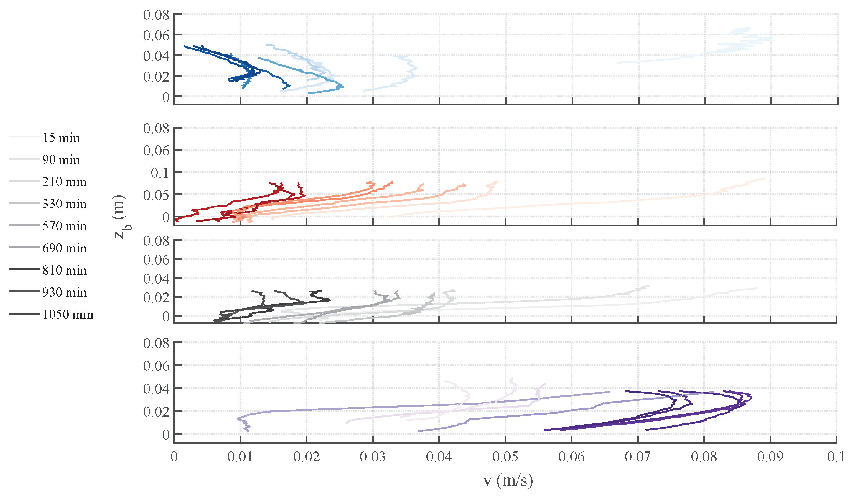
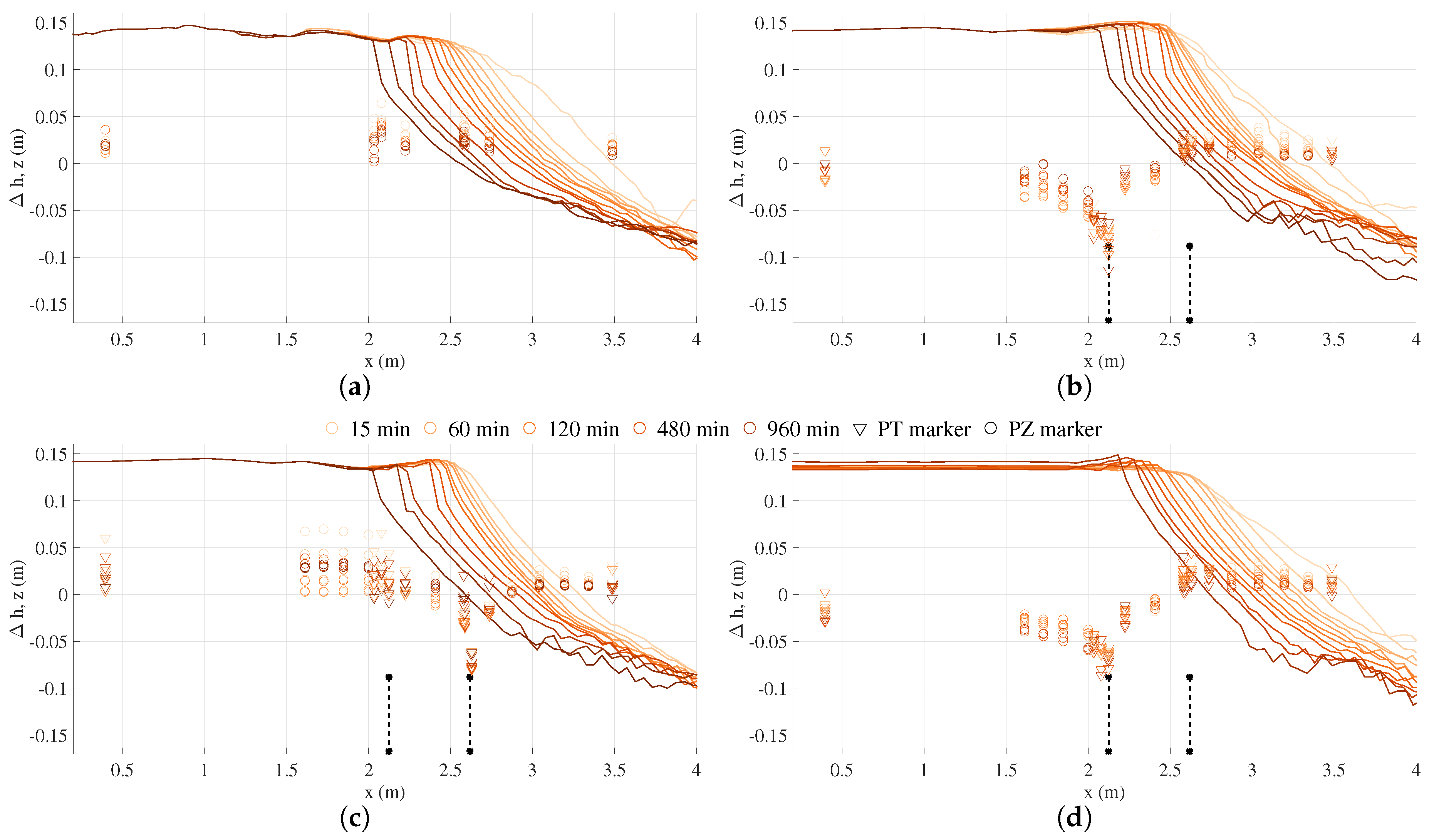
Figure 1. (a) Cross-section of the physical model built in LIC 2D flume with overlapped the plan view of the instruments and drains locations on the shoreface (Detail A.1); (b) detail of drain pipes, piezometers ( P Z ), pore pressure transducers ( P T ) placed inside the sand (Detail A.2); (c) detail of the submerged sill (Detail B); (d) perspective picture of drain pipes and instruments, during installation, with magnification of P Z and P T ; and (e) lateral view of submerged sill, ADVs and wave gauges.
Water 10 01171 g001
Figure 2. Time variation of P T during first time step ( 15 min) for configuration B D S 1 . Circle markers defines the initial (red-filled) and final (grey-filled) points used for signals averaging. Different ordinates limits are used to catch the time evolution of the signals.
Water 10 01171 g002
Figure 3. Spatial variation of water tables at the first step ( 15 min).
Water 10 01171 g003
Figure 4. Significant wave height H s spatial distribution.
Water 10 01171 g004
Figure 5. Power amplitude spectra variation for U N P , B D S 1 , B D S 2 and B D S 1 - B W configurations.
Water 10 01171 g005
Figure 6. Bulk statistics of swash oscillations over time. (a) Wave runup R 2 % (top), R m a x (bottom); (b) Wave setup ( η ).
Water 10 01171 g006
Figure 7. Time evolution of v-component of the velocity vectors for U N P ( Water 10 01171 i001); B D S 1 ( Water 10 01171 i002); B D S 2 ( Water 10 01171 i003); and B D S 1 - B W ( Water 10 01171 i004) tests. z b refers to distances from the bottom, positive upward.
Water 10 01171 g007
Figure 8. Spatial and temporal variation of groundwater table with the relative profiles measured at the end of the selected test step: (a) U N P ; (b) B D S 1 ; (c) B D S 2 ; and (d) B D S 1 - B W .
Water 10 01171 g008
Figure 9. (a) Time-evolution of beach profile measured at the centreline (z, blue gradient lines). (b) Spatial and temporal evolution of bottom elevation changes ( Δ z ) with respect to the initial profile.
Water 10 01171 g009
Figure 10. Comparison between final profiles (a) and bottom changes (b) for unprotected ( U N P ) and protected ( B D S 1 , B D S 2 , and B D S 1 - B W ) cases. The origin of the horizontal axis coincides with the location of the initial shoreline.
Water 10 01171 g010
Figure 11. Sediment transport rates over time for the different configurations.
Water 10 01171 g011
Figure 12. Sediment transport rates ( q s ) and measured profiles ( z b ) at 15 min (a), 90 min (b) and at the submerged bar equilibrium (c) in unprotected conditions.
Water 10 01171 g012
Figure 13. Temporal variation of depth-lines 0.03 m, 0 m, + 0.03 m locations (a) and mean foreshore slope (b) for each configuration from the beginning of each test.
Water 10 01171 g013
Figure 14. (a) Sketch of the main parameters useful for bar description. (b) Temporal variation of crest bar location, x b (left panel) and dimensionless bar crest height, ζ b (right panel).
Water 10 01171 g014
Table 1. Test ID and main bulk parameters of wave attacks.
TestTest ID H s (m) H m 0 (m) T p (s) m 0
UnprotectedUNP0.1870.2061.470.0027
Drain 1BDS10.1830.2061.470.0027
Drain 2BDS20.180.2031.470.0026
Drain 1 + Submerged BreakwaterBDS1-BW0.190.2121.470.0028

