Article

Modelling Spatiotemporal Dynamics of Large Wood Recruitment, Transport, and Deposition at the River Reach Scale during Extreme Floods

by
Andreas Paul Zischg
1,*,
Niccolo Galatioto
1,
Silvana Deplazes
1,
Rolf Weingartner
1 and
Bruno Mazzorana
2
1
Oeschger Centre for Climate Change Research, Institute of Geography, University of Bern, Bern CH-3012, Switzerland
2
Faculty of Sciences, Instituto de Ciencias de la Tierra, Universidad Austral de Chile, Valdivia 5090000, Chile
*
Author to whom correspondence should be addressed.
Water 2018, 10(9), 1134; https://doi.org/10.3390/w10091134
Submission received: 22 June 2018 / Revised: 23 August 2018 / Accepted: 23 August 2018 / Published: 25 August 2018
(This article belongs to the Section Hydraulics and Hydrodynamics)

Abstract

:
Large wood (LW) can lead to clogging at bridges and thus cause obstruction, followed by floodplain inundation. Moreover, colliding logs can cause severe damage to bridges, defense structures, and other infrastructure elements. The factors influencing spatiotemporal LW dynamics (LWD) during extreme floods vary remarkably across river basins and flood scenarios. However, there is a lack of methods to estimate the amount of LW in rivers during extreme floods. Modelling approaches allow for a reliable assessment of LW dynamics during extreme flood events by determining LW recruitment, transport, and deposition patterns. Here, we present a method for simulating LWD on a river reach scale implemented in R (LWDsimR). We extended a previously developed LW transport model with a tree recognition model on the basis of Light Detection and Ranging (LiDAR) data for LW recruitment simulation. In addition, we coupled the LWD simulation model with the hydrodynamic simulation model Basic Simulation Environment for Computation of Environmental Flow and Natural Hazard Simulation (BASEMENT-ETH) by adapting the existing LW transport model to be used on irregular meshes. The model has been applied in the Aare River basin (Switzerland) to quantify mobilized LW volumes and the associated flow paths in a probable maximum flood scenario.

Graphical Abstract

1. Introduction

Riverine floods in many parts of the world are a threat to people, settlements, and infrastructure and thus a major cause of significant losses [1]. Analyzing flood events is therefore a prerequisite for risk management. Floods are triggered by precipitation events of high intensity or long duration. However, the local flood magnitude also depends on catchment characteristics, land use, river morphology, and the status of flood defense measures [2,3,4]. Especially in mountainous areas, the impacts of floods can be accentuated by sediment transport or large wood (LW) transport. Both sediment and LW transport can lead to bridge clogging with subsequent channel outbursts [5]. Concomitantly, bridges may be severely damaged and flood magnitude may be increased in the floodplain [5,6,7,8,9]. If sediment deposition in the river channel and subsequent riverbed aggradation or LW jam formation potentially occur in a specific site, obstruction of bridges due to these processes has to be considered in the prediction of flooded areas and the associated adverse consequences [10]. In addition, the destruction of flood defenses or other infrastructure due to colliding trunks plays a relevant role in flood consequence analysis. The factors influencing the process magnitude and the course of a flood event are often considered in risk analyses by defining different scenarios that potentially lead to an aggravation of the flood and related consequences [11,12,13]. Hence, the amount of sediment or LW is an important aspect in scenario definition and thus risk analysis. These estimations are a prerequisite for the design of flood mitigation measures. Furthermore, it is important to know which processes can occur at a specific point of interest and how these processes will evolve spatially and temporally under different circumstances. Considering sediment dynamics during floods is becoming more frequent in flood risk analysis. In recent years, various simulation models have been developed for modelling this process [14,15,16]. In contrast, methods and simulation models for assessing the recruitment, transport, and deposition of LW during floods still need to be substantially improved. The topic of in-stream LW has been extensively investigated within the domains of ecology, geomorphology, and hydromorphology. Here, the focus is placed on the relevance of wood for river habitats and river morphology [17,18,19,20,21,22,23,24], wood budgets [25,26,27,28], wood storage [29,30], and wood transport rates in rivers [23,31,32] in the long term. Only a few studies describe methods for quantifying LW volumes and fluxes in rivers in the short term [33,34,35,36,37], e.g., by remote sensing [38,39,40], radio frequency identification (RFID) and Global Positioning System (GPS) techniques [36,41], time-lapse photography [34], or video monitoring [42,43,44]. On the other hand, the spatiotemporal dynamics of LW in rivers has been analyzed from the risk management perspective with a focus on extreme floods only in recent years. Comiti et al. [45] stated that the current knowledge of LW dynamics (LWD; i.e., recruitment, transport, and deposition) during high-magnitude floods is still limited since extreme floods are, by definition, rare events and thus the opportunity to study these processes in reality is very limited. Practically, during extreme weather events, observing and monitoring hazardous processes is logistically complex and temporally challenging. Another reason for these knowledge limitations is that these highly complex processes differ substantially across river basins [23,27,45,46,47,48]. Due to remarkable variability of catchments in terms of land use, geology, forested area, and river hydromorphology, empirical estimations of LW volumes during large floods are uncertain. Furthermore, other geomorphologic processes play an important role in wood recruitment. The flood hydrograph is one of the main factors influencing LW volume [49]. Thus, transferring the analysis from one catchment to others is questionable. In addition, the recruitment of trees and entrainment into the river flow is influenced by riverbank erosion, landslides in forested areas near the riverbed, and debris flows bringing eroded trees from tributary catchments into the main river channel [45,50,51,52,53]. Moreover, small mountain torrents, wide gravel-bed rivers, and regulated rivers exhibit pronounced differences in LW dynamics [45].
In summary, LWD are complex and consist of different subprocesses. Different models for simulating LW transport and deposition have been developed so far. Abbe et al. [54] described LW patterns and processes of LW and woody debris at the micro scale, with a focus on jam formation. Amicarelli et al. [55] and Albano et al. [56] modeled LWD with a smoothed particle hydrodynamics approach. Bragg et al. [57] modeled the ecological disturbance in riparian forests at the single tree scale. Bocchiola et al. [58] presented a simplified numerical approach to model LW transport in one dimension (1D). Models that consider the movement of single trees on the basis of a hydrodynamic two-dimensional (2D) model have been proposed by Mazzorana et al. [59] and Ruiz-Villanueva et al. [60]. The latter is, to our knowledge, the most complex model for simulating LW transport, deposition, and jamming at bridges or other obstacles. The model is implemented in a 2D hydraulic model (Iber) that solves the shallow water equations with a finite volume method [61,62]. The LW transport model simulates incipient motion of single pieces of wood, performing a balance of the forces acting on it. Interactions between logs and the channel configuration and among the logs themselves, with subsequent influence on the hydrodynamics, are also taken into account. The logs are represented by cylindrical objects. This model is the most advanced in terms of process representation at the micro scale. However, the LW fluxes at the upper boundary condition have to be estimated. In contrast, Mazzorana et al. [59] presented an approach that also considers the recruitment process. The erosion of standing trees is considered by analyzing the hydrodynamic forces. The transport of the logs is coupled with a 2D hydrodynamic model and the dynamics of single floating wood are computed on the basis of flow forces [63,64,65]. However, the coupling is of unidirectional type and therefore the influence of wood jams on the hydrodynamics is neglected. The logs are represented by points and the interaction between the logs and obstacles and among the logs themselves is more generalized than in the approach of Ruiz-Villanueva et al. [60]. However, this approach is, to our knowledge, the only one that considers the whole process chain of LW recruitment, transport, and deposition. The approach of Mazzorana et al. [59] requires the locations of standing trees or lying trees or logs as input data. Thus, the trees in floodplains have to be localized and classified, and their volume must be estimated. For this task, some approaches have only recently been developed. Besides the interpretation of aerial images [66] or geographic information system (GIS) analysis [26,59], a number of approaches for single-tree detection and classification on the basis of Light Detection and Ranging (LiDAR) data have been published [67,68,69,70,71,72,73,74,75]. These approaches significantly facilitate the preprocessing of the input data needed for LW transport models.
In summary, if risk management options have to be designed at a specific point of interest where LWD are expected to significantly influence the flood process, engineers can use simulation models explicitly dedicated to analyzing the clogging of LW at bridges while considering the interactions between the logs and a two-way coupling with the hydrodynamic model (i.e., [60]). Regarding the estimation of upper boundary conditions for simulations of the clogging process, there is a lack of methods for (a) estimating potential LW volume standing in the flood influence zones upstream of the object at risk, (b) assessing the spatiotemporal dynamics of LW within a flood event (i.e., a time series of wood fluxes), and (c) identifying the most relevant recruitment areas that deliver LW to the point of interest (e.g., a planned bridge or weir). The latter includes the transport and deposition processes along the river reach. However, a single tool for answering all these questions is still missing. In particular, estimating wood load in terms of LW volume during extreme floods is difficult, because statistical methods are not feasible due to the rarity of observation data.
The main goal of this work was therefore to develop a tool for quantifying incoming LW fluxes at a specific point of interest in a river network as a basis for the design of wood-retention structures in a river basin. This requires the full consideration of LWD—from recruitment to transport and deposition—along the river reach upstream of the point of interest. Apart from the approach of Mazzorana et al. [59], there are no applicable or extendable models to cover the full “process cascade” at the required spatial scale. However, the latter approach is implemented in raster-based software. As modelling LWD requires high spatial resolution, the raster approach limits the application of the model to restricted sizes of the study area. The approach of Mazzorana et al. [59] does not allow simulating LWD at the river reach scale with the required spatial resolution.
Thus, the main research question here relates to the applicability of a full model chain to simulate LWD during an extreme flood at river reach scale. Our hypothesis is that implementing the model in a vector-based, object-oriented modelling approach on the basis of irregular triangular computational meshes allows simulating LWD at the required scale and spatial resolution. Consequently, this requires modelling LW as objects (floating logs). Hence, the secondary research question relates to the development of a tree detection and volume estimation approach.
Accordingly, this paper first describes the general framework for LW recruitment and transport modelling. Second, the model is evaluated by comparing the simulation results with well-documented flood events. After this evaluation, a model application for assessing LWD during an extreme flood event is described. Finally, the results are discussed and conclusions on the use of the proposed model in flood risk management are drawn from the model evaluation and application.

2. Methods

The presented approach is based on the following steps: detection and characterization of trees, hydraulic modelling, modelling of the recruitment of LW, and modelling of the transportation and deposition processes. Hence, this section is structured along this concept (Figure 1). First, we present the overall modelling approach. Herein, an introduction to the basic framework of LWD simulation is given. Second, the method for identifying single trees in forested areas and classifying the vegetation is described. After an explanation of the procedure for simulating hydrodynamics with Basic Simulation Environment for Computation of Environmental Flow and Natural Hazard Simulation (BASEMENT-ETH), we describe the implementation of the relevant processes of LW dynamics, i.e., recruitment, mobilization, transport, deposition, and entrapment at bridges. Herein, the basic idea and the implementation of the model are explained. The whole procedure was implemented in a set of functions programmed in R (LWDsimR (see Supplementary Materials)). The software was developed in the framework of the present study.

2.1. Basic Framework of LWD Modelling

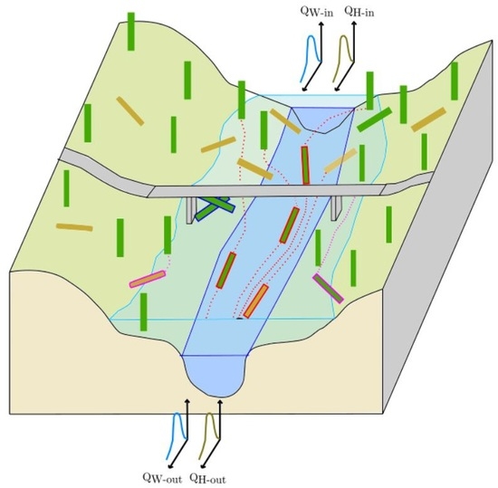
The basic concept of LWDsimR follows the approach of Mazzorana et al. [59] and was extended with a tree recognition and classification module. LWD during a flood is simulated in a spatially (upper, lower, and lateral boundaries) and temporally (duration of the event) delimited system. Water flow entering the system at the upper system boundary and leaving it at the lower system boundary is simulated by a two-dimensional hydrodynamic model. The vegetated area in the system is represented in single-tree resolution. The trees are extracted from LiDAR data and classified on the basis of forest inventory data. Single trees are represented as cylindrical objects, which may have rootstock in the form of a disc and a specific diameter. Branches, crown, and rejuvenation are neglected. Every tree is considered by the model as a point feature in space with certain attributes describing its characteristics and status during the simulation time. During the simulation, every tree has a “status” that defines whether it is rooted, lying, transported, or jammed at a bridge. Under given conditions at every time step, standing trees can therefore be recruited (eroded and mobilized) and transported into the channel. The lying trees (greenwood and deadwood) can be transported by the flood, depending on the hydrodynamic conditions. During the simulation, the trees can be deposited, remobilized, or entrapped at bridges, or can leave the system at the lower system boundary (LSB). Only trees that are standing in the influence zone of the flood (flooded areas) and are directly influenced by hydrodynamic forces are considered for recruitment. All trees outside of the flooding perimeter are neglected or have to be inserted into the system border (e.g., contributions of tributaries or provided by hillslope processes). The main input data needed for simulation are hydrographs at the upper boundary conditions, digital surface and elevation models, and data about local forest characteristics (forest inventory). While the hydrodynamic simulation is done with BASEMENT-ETH, LWD simulation and postprocessing are performed with LWDsimR.

2.2. Identification and Classification of Trees

The detection of single trees in the forested areas is based on digital surface models (DSMs) and digital elevation models (DEMs) with a spatial resolution of 0.5 m [76]. A normalized surface model (NSM) is calculated by subtracting the DEM from the DSM. The forested area is defined by a predefined vegetation mask extracted from the land cover map LK25 of the Federal Office for Topography (SWISSTOPO). It is assumed that tree crowns are represented as local maxima in the NSM [77]. Therefore, they can be detected using a moving window approach. Here, we used a window of 3.5 × 3.5 m. A grid cell is defined as a local maximum if all of its neighbors in the window have a lower height value. To be identified as a tree, a cell has to exceed a predefined minimum height, in our case 3 m. This approach is sensitive to the size of the window. A small window generally leads to the detection of more local maxima, which can cause erroneous multidetections of large trees with big crowns and several smaller tops. With an increasing window size, the risk of multidetection decreases, but smaller and dense standing trees might be neglected. Hence, the size of the window must be chosen carefully and with regard to the prevalent vegetation structure. We used sample areas for calibration in which we measured the location and height of each tree.
After detecting the trees, the necessary attributes of every tree, namely diameter at breast height (DBH), tree height, diameter of rootstock, forest structure [78,79], and slope, are determined. The height of the trees can be directly derived from the NSM, whereas DBH has to be calculated on the basis of height using a regional tariff function [80]. The diameter of the rootstock can be defined as a multiple of DBH with a factor between 2 and 3 [38] or 5 [59]. The attribute “structure” represents the vegetation structure concerning the age and density according to [59]. The tree density (443 trees with a DBH ≥ 12 cm per hectare) was delineated from the forest inventory of the region “Northern Alps, West” [78,79]. Moreover, it is necessary to determine whether a tree is standing in an area unit with predominant young vegetation and if the tree density in this area unit is above or below a predefined threshold. The attribute “slope” determines, over a threshold, whether a tree is standing in a steep or rather flat area. The threshold for defining steep slopes is 25°. Subsequently, we estimated the volume of every tree according to the function proposed by Denzin [81] (Equation (1)). We used a form factor f of 0.5. l is the tree height.
v o l =   π 4   ×   D B H 2   ×   f   ×   l
The location of deadwood is generated as a set of random points within the forested area. The amount of deadwood (i.e., the point density for the study region) can be estimated on the basis of forest inventories. In our study, we used a density of 24 trees/hectare. We deduced the length and diameter of the deadwood from the relative frequency distribution of samples from field studies in the riparian forests of Belp, Elfenau, Rubigen, and Uttigen (n = 149). Finally, the generated greenwood and deadwood are merged into a point shapefile with a unique ID and the corresponding attributes.

2.3. Hydrodynamic Simulation

For the hydrodynamic simulation, the freely available BASEMENT-ETH software was used [14]. BASEMENT-ETH consists of 2 numerical subsystems: BASEchain for 1-dimensional numerical simulations of river reaches based on cross-section and BASEplane for 2-dimensional numeric simulation of river reaches and flood plains based on an unstructured mesh. In both subsystems, sediment transport can be considered [14]. This tool basically solves shallow water equations. The topography is represented in an unstructured flexible mesh, whereas single triangles have an assigned roughness represented by Strickler values. During the simulation, flux takes place on the edges between 2 elements in finite volume methods and the water level and velocity in the x and y directions are calculated. This hydraulic model has been extensively used and validated in the study area [82,83,84,85,86,87]. The calculated flow variables for different time steps form the basis for the subsequent simulation of LW dynamics.
The simulation on the basis of an unstructured mesh offers some benefits for LWD modelling. In comparison to approaches based on regular grids, the size of the study area can be extended without losing too much detail within the river channel. Thus, the approach of irregular meshes is expected to be more adaptable, especially at locations with relevant discontinuities [56]. In contrast, the approach of Mazzorana et al. [59] for LWD simulation is based on regular grids. Hence, there is a trade-off between the spatial resolution of the grid and the extent of the study area. As a consequence of increased grid size, a loss in the robustness of in-stream LW transport simulation has to be expected. Therefore, here we adapted the original approach of Mazzorana et al. [59] for LWD simulation to be used on irregular meshes.

2.4. LWD Simulation

The following section explains the functionality of LWDsimR in detail. The program was written in the R programming language [88]. The transport simulation was extended with capabilities for input generation (tree identification and classification). The results of hydrodynamic simulations were used as the basis for the LWD simulation. The 2 models were unilaterally coupled and the influence of LW on the hydrodynamics was neglected. However, a simplified approach for considering the retention of LW volume by bridges was implemented.
Basically, the simulation of LWD is calculated in 2 nested loops. The function of the outer loop is to load the results of the different time steps from the hydrodynamic simulation (flow depth and velocity in the x and y directions) into the model. The function of the inner loop is to calculate the processes of LWD in a specific number of time steps during one time step of the hydrodynamic simulation. Hence, the number of iterations of the inner loop defines the number of time steps and therefore the temporal resolution of the LWD simulation. This procedure allows LWD to be simulated with a higher temporal resolution than the hydrodynamics.
During every time step of the inner loop, the following procedure is executed to calculate the LWD processes:
  • Localization: For every tree, its closest 3 mesh-nodes of the hydrodynamic model are identified. On these nodes, the hydrodynamic conditions of the particular time step are read out. The conditions are interpolated at the position of the tree using the inverse distance weighting interpolation method.
  • Recruitment and mobilization: Whether standing trees are standing or have fallen into the channel is checked. For standing trees, the hydrodynamic forces are analyzed to estimate the recruitment. For uprooted trees, the recruitment analysis is not needed and the flow conditions are analyzed; only recruitment processes from soil erosion in the influence zone of the flood are considered. Lateral erosion of river banks and subsequent river widening or other changes of the channel morphology are not considered. Since there is still a lack of detailed knowledge with respect to possible recruitment mechanisms, a probabilistic approach is considered. Depending on the hydrodynamic forces acting on a tree, a recruitment probability is determined on the basis of the vegetation structure and the local slope according to [59]. In a first step, the hydraulic impact C is calculated on the basis of flow depth h and flow velocity U (Equation (2)).
    C = h   ×   U 2 2 g
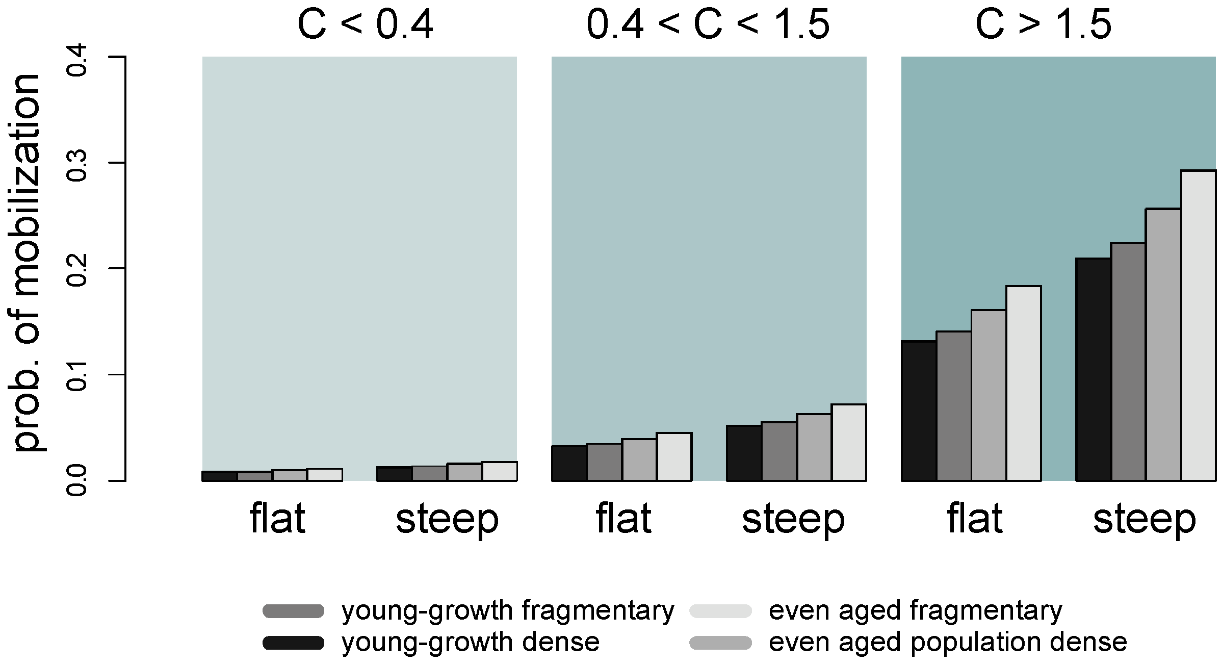
  • On the basis of the classified hydraulic impact, the wood structure, and the slope, a probability factor of recruitment is assigned (Figure 2). The probability of mobilization is calculated for each time step, divided by the total number of time steps. For each tree, it is randomly defined if the status of the tree changes from “standing” to “recruited,” depending on the assigned probability. A “recruited” tree is defined as an uprooted tree that has fallen due to hydrodynamic forces.
  • Entrainment, transport, and deposition: For all lying trees (uprooted greenwood and deadwood), it is checked whether the conditions for entrainment are fulfilled. For simplicity, it is assumed that the density of all trees is lower than 1 and their orientation is parallel to the flow. Interactions between trees and breaking of logs are neglected. The transport process can take place under floating or rolling/sliding conditions [89]. Depending on these conditions, the transport velocity differs from a velocity equal to the streamflow for floating trees to reduced velocity for sliding or rolling trees. For a comprehensive description of the physical foundations of the transport dynamics, we refer to the literature [59]. Using the information about velocity and flow direction, the new positions for every transported log are calculated for every time step. A transported log can be deposited at a particular time step if the conditions for transportation are not fulfilled anymore, and it can be remobilized at a later time step. Transported trees that are not deposited or entrapped at a bridge reach the lower system boundary (LSB) and are not considered in the further simulation.
  • Bridge clogging: Bridges can optionally be considered in the model as polygon geometries with information about their height above the riverbed and length. If 1 or more of the 3 closest mesh-nodes of a transported tree lies within such a polygon, it is assumed that the tree is passing a bridge. In this case, it can collide with 1 or more piers or interact with the bridge deck and cause clogging [90]. As a simplification, the specific bridge structure and the flow conditions are neglected. Furthermore, if log jams are formed, they do not interact with other trees and cannot break. With regard to the randomness of this process and the lack of physical knowledge, a probabilistic approach is applied. According to [90], the probability of a log being jammed at a bridge is the sum of all blocking probabilities on single bridge elements. The blocking probability for the piers is calculated following [91] since only the bottom width and log length are considered in the equation. The clogging probability at the bridge piers is calculated according to [92] (Equation (3)) and at the bridge deck according to [93] for trees with (Equation (4)) and without (Equation (5)) rootstocks. The total blocking probability of a tree at a bridge is the sum of the single probabilities. A random generator is used to determine, with the given probability, whether a tree is jammed or passes the bridge normally. For a detailed description of the clogging probabilities, we refer to [91]. This feature considering LW retention by clogging is optional.
    p r o b p i e r   =   1 15 +   2 l 15   ×   B m i n
    p r o b d e c k   l o g   =   3.5 + 2.56   ×   h + d R 2 H
    p r o b d e c k   r o o t   =   0.074 + 0.88   ×   l B m i n   ×   h +   d 2 H
Where l is the log length; Bmin is the minimal distance between bridge piers; h is the flow depth; H is the distance between river bed and lowermost edge of the bridge; dR is the diameter of rootstock; d is the diameter of log.
The results are saved and the LWD processes are calculated again for the next time step. The final result consists of a 3-dimensional array showing the status and location (x, y coordinates) of each log. From this, the tracking of the logs during the simulation, a video of the simulation, or the analysis of the LWD dynamics along the river reach can be derived. The volume of LW is quantified in solid form, i.e., considering the wood mass only.

2.5. Model Test

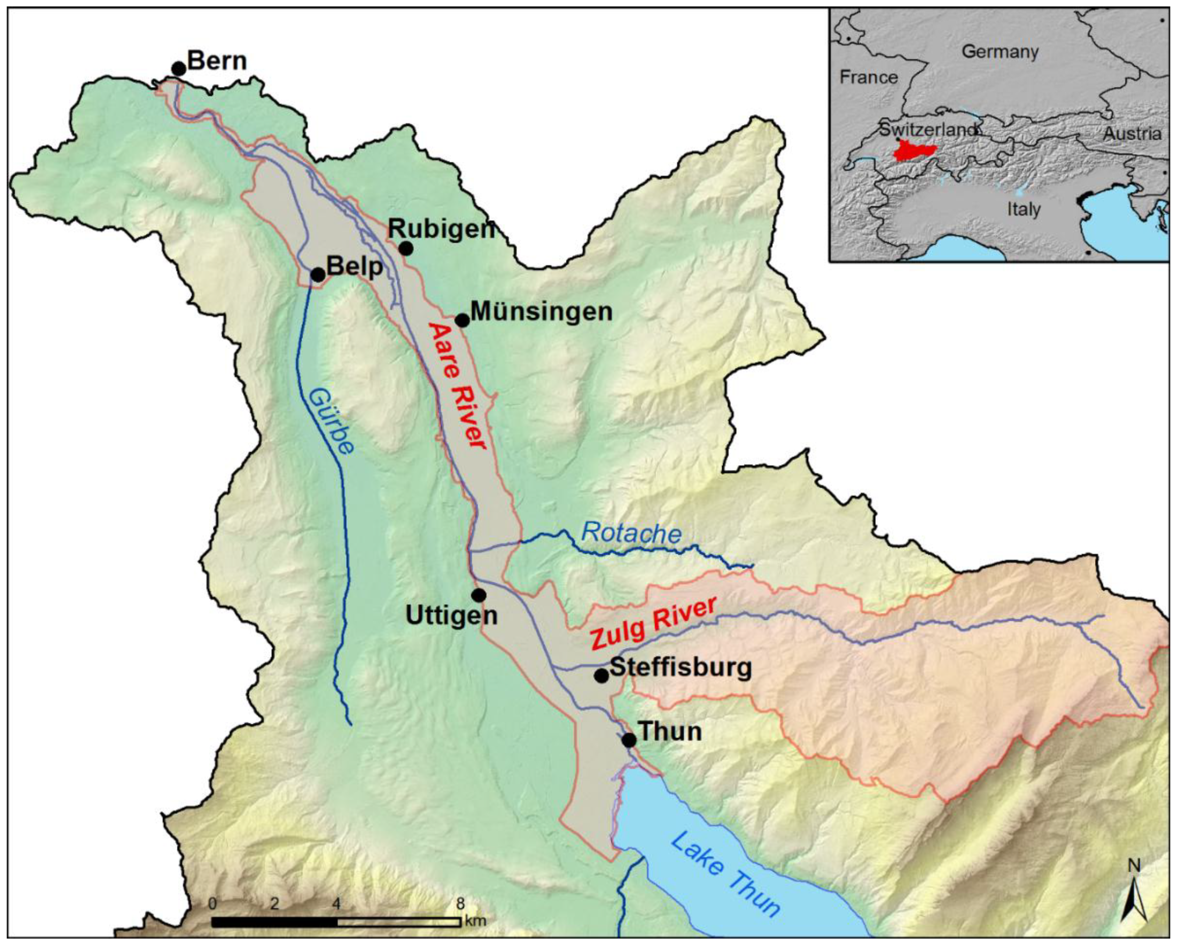
To test and validate LWDsimR, we compared model runs with observations. We reconstructed 2 well-documented flood events with the model. The first test was done in the Aare River reach from Thun to Bern, Canton of Bern, Switzerland (see Figure 2). We reconstructed the flood event of August 22, 2005, and compared the simulated LW volume at the lower system boundary with the observed volume. During this flood event, the Aare River had a peak discharge of 605 m3/s and an estimated return period of >150 years [94]. Approximately 2300 m3 of loose and 600–900 m3 of solid woody material blocked the weir [95]. The flood event led to inundation of the Matte district, generating 50 × 106 Swiss Francs of damages [96]. Second, we tested whether the LW input delivered from the tributary Zulg River in the flood event of June 7, 2015, could be transported toward Bern as documented. Here, we first modelled recruitment and transport within the Zulg River catchment. Subsequently, we used the LW volume coming from the tributary as input to the main river and modelled the transport of LW along the Aare River toward Bern.

2.6. Modelling LWD during an Extreme Flood

Large quantities of LW transported by the Aare River to Bern pose a severe problem, since clogging of the Mattenschwelle weir can lead to severe inundation of the Matte district in the city of Bern due to backwater effects. This happened during the flood event in 2005. For sound risk management, knowledge about LWD in the Aare River and an estimation of the maximum volumes of woody material in the worst case scenario are paramount. Therefore, the focus of our attention in modelling an extreme flood scenario that explicitly takes into account LWD is the city of Bern (see Figure 3). The main LW recruitment areas are located in the floodplain of the river Aare between Thun and Bern. In this floodplain, we considered LW recruitment due to erosion of root wads by hydrodynamic forces. Hence, we simulated LW dynamics in the Aare between Thun and Bern during an extreme flood event. This is a flood scenario of a probable maximum precipitation event [97], with a peak discharge of 1100 m3/s and a duration of 40 h. The outcome of the hydrodynamic model has a temporal resolution of 20 min and the time step of LWDsimR is set to 5 s. Bridge clogging in the upstream river reaches is neglected, because only pierless and high bridges span the Aare River. The Zulg River tributary can potentially deliver relevant LW quantities to the main river. The confluence of the Zulg and Aare rivers is in Steffisburg, 3 km downstream of Thun. It is considered an important source of woody material and therefore was modelled separately first. Logs transported from the upper Zulg catchment to Steffisburg were used as input for the simulation of LWD in the Aare River. The other tributaries of the river downstream of Lake Thun do not have any relevant forests in the flood influence zones and thus do not deliver LW to the main river. LW delivered by the tributaries upstream of Lake Thun is entrapped by the lake and thus is not relevant to the point of interest.

3. Results

The reconstruction of the flood event in August 2005 resulted in a LW volume of 1774 m3 at the lower boundary condition in Bern. This is remarkably higher than the observed volume of 600–900 m3. However, the latter takes into account clogged wood only. The volume of LW that passed the weir during the flood is unknown. In contrast, the simulated volume represents the volume of LW that passed the LSB. Thus, the results of simulated LW volume must be above the observed value.
The second model test showed that during the 2015 flood in the Zulg River, an LW volume of 343 m3 was recruited in the catchment and transported to the confluence with the Aare River. This is in line with the estimation of <<600 m3 that was observed and documented by public authorities [98]. In contrast to our simulation, landslides also contributed to LW during this flood in the Zulg River catchment. Here, we do not consider the recruitment of LW by landslides, therefore the simulated volume has to be lower than the observed volume. Logs coming from the Zulg tributary follow the thalweg of the Aare River and no implausible deposition of LW along the river banks was simulated. Along its flow in the Aare River, LW coming from the Zulg River was dispersed into a more or less dense layer. From the total LW volume of the Zulg River, 98.5% was transported to Bern in this test case. Only a small volume of LW was deposited in the confluence between the Zulg and Aare rivers. This is in line with observations along the Aare River after this flood event.
Applying the model to an extreme flood event gives the expected LW volume at the point of interest, in our case the Matteschwelle weir in Bern. An overview concerning the volume of the simulated LWD is shown in Table 1. From the alluvial forests between Thun and Bern, with a total stock of 112,661 m3 in the direct flood influence zone, 11,841 m3 was recruited in the simulation; 7288 m3 was deposited within the system and did not reach Bern, whereas 3933 m3 was transported through the system toward the LSB, including the 343 m3 from the Zulg River catchment.
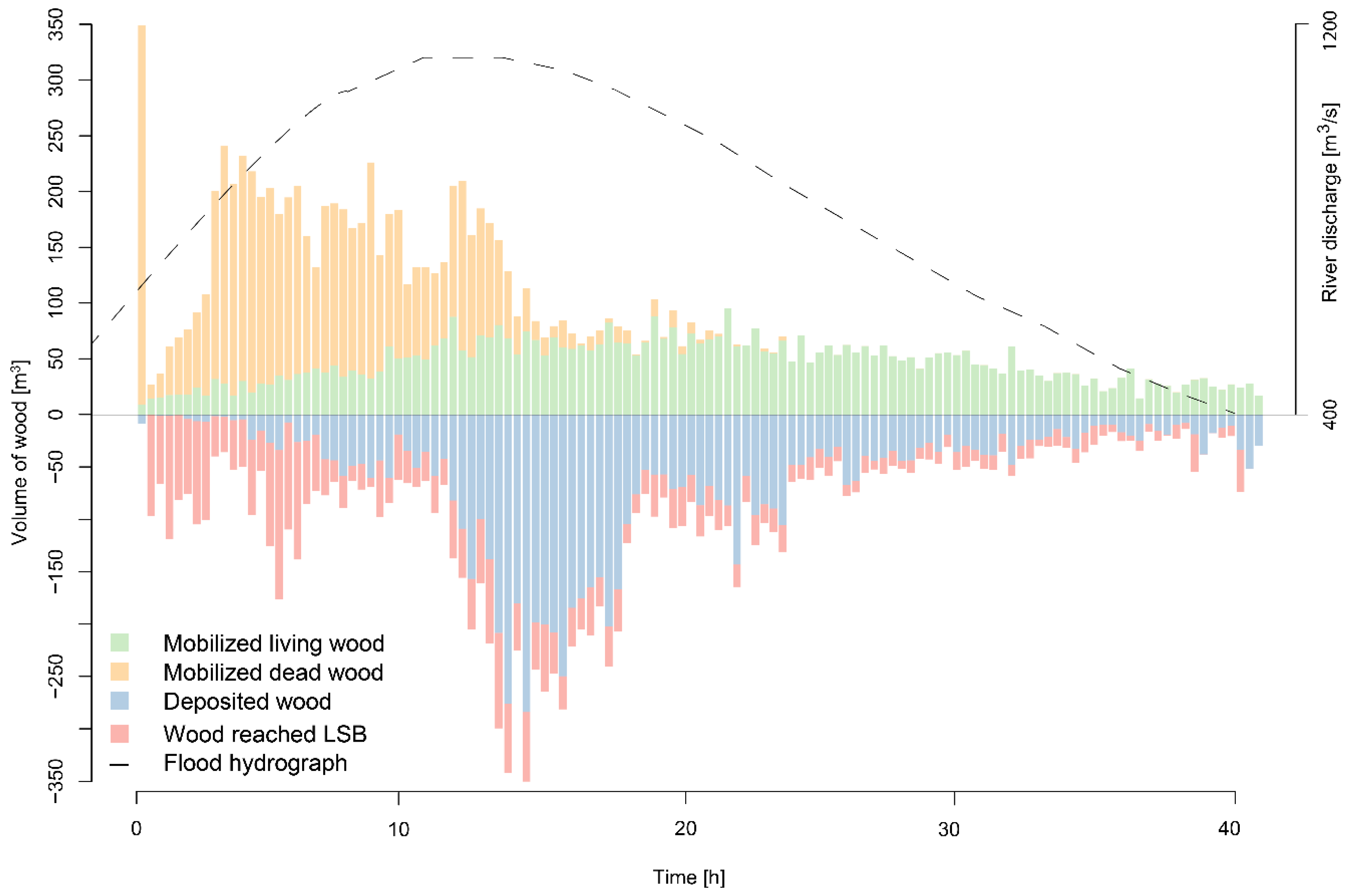
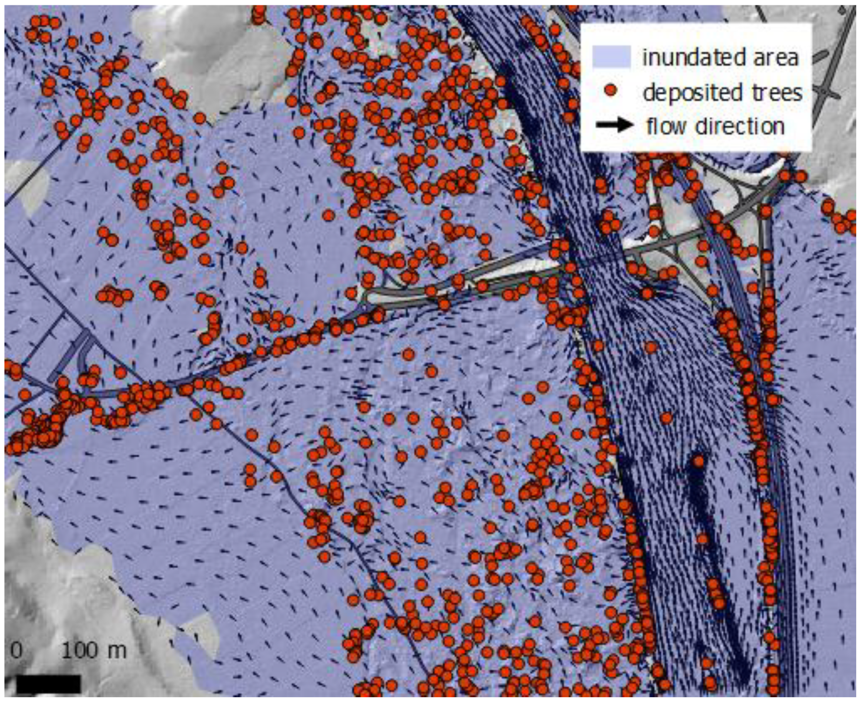
The temporal distribution of the simulated LWD in the Aare River is shown in Figure 4. The hydrodynamic simulation starts with a bankfull discharge and partially flooded alluvial forests within the river bed as the initial condition. Thus, the initial recruitment rate is very high and there is a high share of deadwood. The mobilization rate soon falls to 25 m3/20 min and then increases again with the rising limb of the hydrograph. The share of greenwood increases, whereas the recruitment of deadwood is reduced constantly over time. The mobilization rate peaks at 250 m3/20 min after 5 h with flooding of the alluvial forests in the floodplain. The mobilization rate drops after the peak discharge is reached after 14 h. LW reaches Bern in 2 pulses; the first pulse occurs 5 h after the simulation start. A decrease of the rate follows before it starts to increase again around peak discharge and peaks a second time at hour 13. After a further peak, it decreases strongly. In all, 61% of the mobilized wood is deposited within the system, mostly on spots close to artificial buildings in the floodplains, such as driveways to the road that bridge over the Aare River. These hydraulic obstacles that perpendicularly cross the floodplain also act as an obstacle for LW, as well as the highway that is partially built on an earth dam (Figure 5).
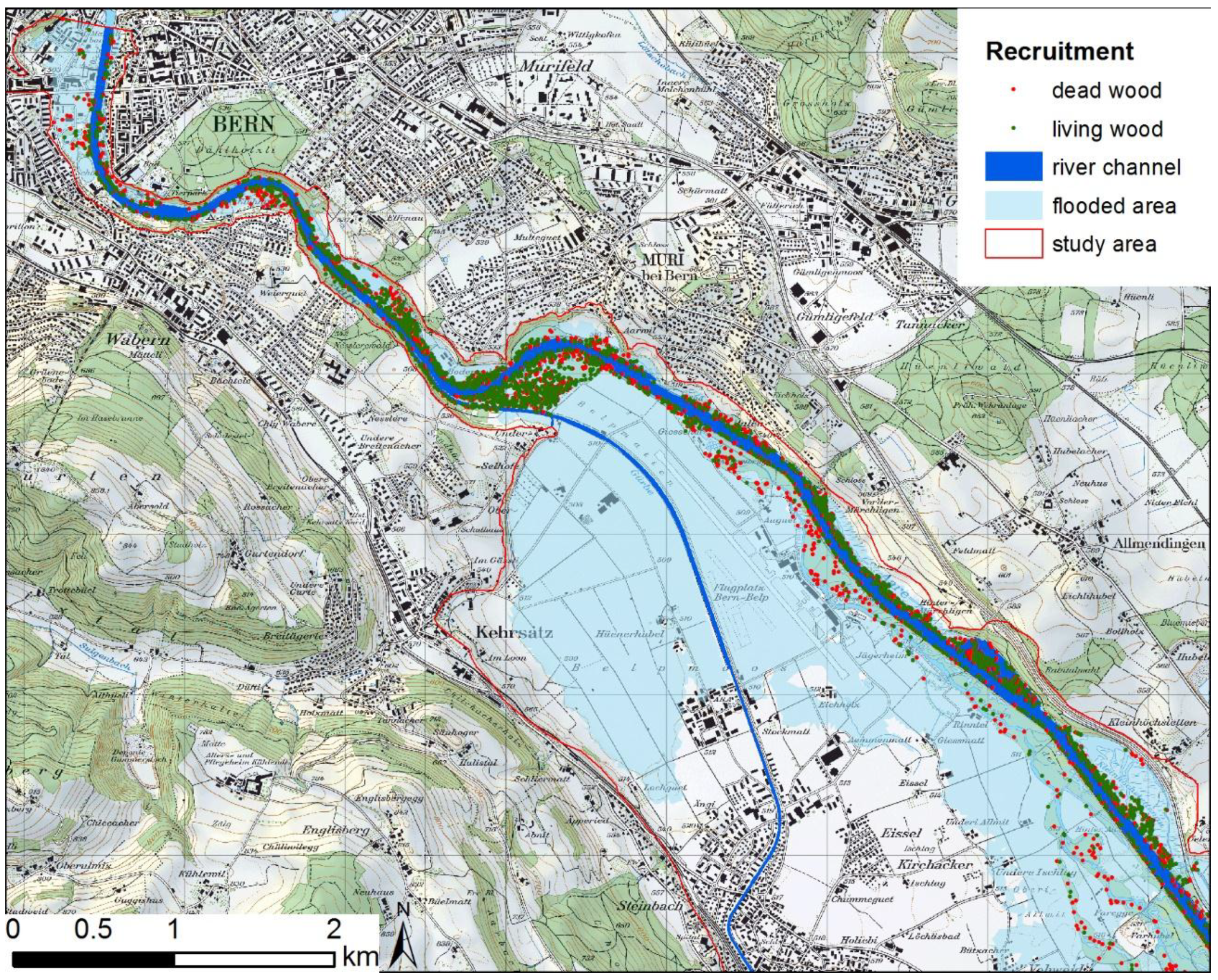
The recruited trees are mostly located along the banks and dams and close to the main channel. This is especially valid for the recruitment areas of LW that reach Bern (Figure 6). Trees located on banks, islands, and areas close to the main channel are most exposed to the hydrodynamics. Once LW reaches the main channel, it can be transported over long distances without being deposited. Only a few selected alluvial forests (Elfenau, Zopfen, Raintalau, and Vorder Jaberg) deliver LW that reaches the LSB. The LW delivered by the Zulg River is transported to Bern.
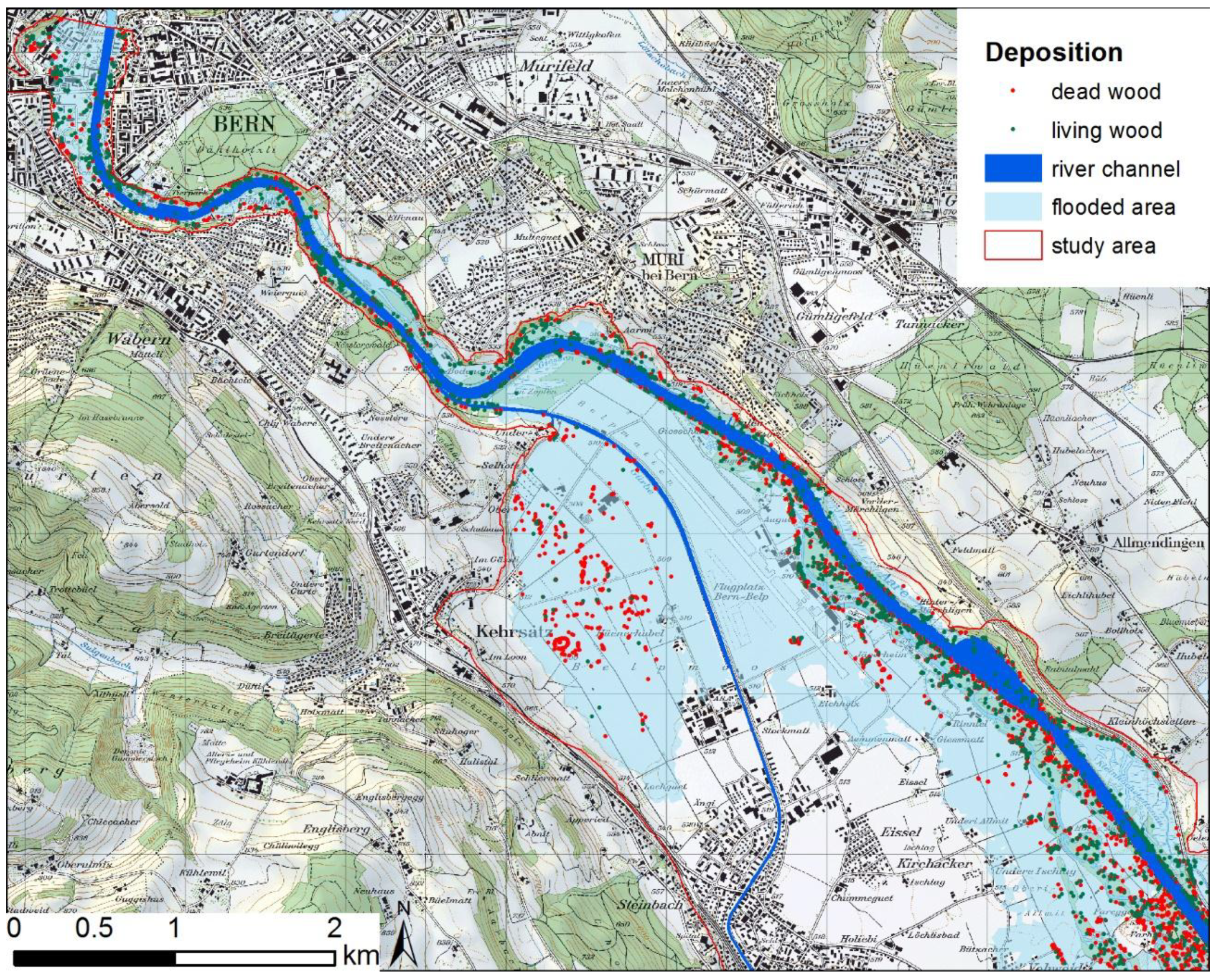
The spatial pattern of the deposition process is different from that of the recruitment process, although deposition is also simulated along the whole river reach. The simulation of LW deposition reveals much more scattered and spotty patterns, with relevant depositions in particular areas. This can be clearly seen in the deposition map in Figure 7. Important locations for deposition of LW within the floodplain are the Aare River bridge near Rubigen (see Figure 5), the heightened highway between Rubigen and Münsingen, the railway bridge near Uttigen, and several spots mostly along the banks or edges of the wetted area. Major depositions are simulated mainly on 2 spots along the highway north and south of the bridge with different deposition patterns. North of the bridge, the woody material was deposited along a zone 400 m in length with shallow water depth, whereas south of the bridge the deposition accumulated on a single spot on the highway. Other specific deposition spots can be found on the left- and right-hand sides of the bridge in the upstream direction. Deposition of smaller volumes occurred in the entire floodplain.

4. Discussion and Conclusions

Comiti et al. [45] raised the question of whether we are able to reliably and quantitatively predict LW recruitment, transport, and deposition within a given river basin during a selected flood scenario of a given magnitude/frequency. In this paper, we presented the LWDsimR modelling tool, which enabled us to answer this question quantitatively to a certain extent in the Aare River basin upstream of Bern, Switzerland.
With the presented approach, it is possible to quantify LW dynamics as a better-informed guess. The procedure could help to estimate the amount of LW volume at a specific point in a river system, especially in areas where no flood events occurred, which helps to assess LW volume empirically by analyzing past events. Implementing the simulation model on an irregular computational mesh allows the simulation of LWD in larger areas, i.e., at a river reach or basin scale. In comparison, a raster-based approach would be limited by the trade-off between spatial resolution and extent of the study area.
The comparison between the simulated and observed volumes of LW at Bern during the flood event of 2005 shows that the model may overestimate predicted LW volume. Despite the uncertainties in the observation, the model tests showed that the approach is applicable to river reaches up to 30 km in length. Moreover, the model correctly simulated the transport path of LW delivered by tributaries in the main river.
In comparison to the LW volume that obstructed the weir in Bern during the flood of 2005, the LW volume to be expected in a worst case flood is considerably higher. A flood event of a probable maximum precipitation scenario produces threefold more LW than the hitherto known most extreme flood. However, it can be assumed that the simulated LW volume transported to the LSB in Bern is rather an upper limit for several reasons. First, the total amount of recruited trees in the floodplains is likely to be overestimated due to high flow depths but relatively low flow velocities. The implemented recruitment algorithm gives large weight to flow depth. Second, a significant part of the recruited wood is not deposited within the system and therefore reaches the lower system boundary at Bern. Standing trees often function as flow obstacles for floating trees. This is not considered here. Moreover, if one flood event occurs, a share of the forest stock will be transported out of the floodplains. A subsequent flood of the same magnitude will have less LW available for recruitment. This leads to the presented approach being sensitive to the date of the forest inventory, i.e., the date of the LiDAR scan. Regarding the recruitment areas, it must furthermore be considered that the Zulg tributary likely plays a considerably more important role than in the simulation results because of the highly probable activity of landslides during an extreme flood.
Nevertheless, the simulation allows the identification of areas prone to recruitment processes of LW due to soil erosion by hydrodynamic forces and shows the ability to transport recruited logs from source areas over long distances to the LSB. Therefore, from a forest management point of view, it may be worthwhile to closely inspect the identified areas, especially those in the upstream vicinity of the point of interest, and to consider preventing massive recruitment of LW.
However, the validation and application of LWDsimR showed some limitations of the tool. The recruitment process is based on a probabilistic approach. Future developments should implement physical-based approaches that fully consider the hydrodynamic forces on vegetation and the resistance of vegetation. Furthermore, we cannot validate the number of recruited trees, because only LW volumes are given in the observation data. Moreover, the clogging process at bridges could not be validated at the time of the study. In LWDsimR, this process is considered only for the purpose of LW budgeting along the river reaches. The modelling of the clogging process has to be improved in the future. Recently, some experiments showed possible ways to improve the modelling of this process [99,100,101,102]. For this question, we recommend using more detailed and fully coupled models, i.e., those in [60].
Another open question is the transferability of the model to smaller alpine rivers and torrents. In rivers with a width on the order of a tree length or less, the transport module may overestimate the deposition and underestimate the transportation of logs toward the lower system boundary. Underestimation may also be caused by neglecting other processes like sediment transport and morphology changes during the flood. Furthermore, it has to be noted that the model neglects the input of LW into a river reach by debris flow from tributaries, by landslides, or by bank erosion and the remobilization of LW that was deposited in the channel during previous floods. These recruitment processes play an important role [52,103,104,105] and have to be implemented in future versions. Thus, future developments should focus on modelling LW recruitment by these geomorphic processes. Moreover, the uncertainties in the model and the sensitivity against input data and model parameters should be analyzed thoroughly in the future. For this, implementing a parallelization scheme in the model is a prerequisite. Another limitation of the model is the requirement of reliable input data, i.e., single trees with their locations and different characteristics. These data are lacking in many regions, and hence transferability may be limited to regions with available data.
Overall, the simulation results of the LW dynamics, both the temporal and spatial dynamics, in a river reach during an extreme flood event provide important information for flood risk management. LWDsimR allows the expected volume of LW on a certain point in the river basin to be assessed by considering the actual conditions of vegetation and a specific flood scenario. This provides a basis for the design of bridges or wood-retention structures and for quantitatively assessing LWD during a worst case flood. Thus, model experiments with LWDsimR could provide a range of values of LW delivery under different flood magnitudes, providing a basis for assessing catchment behavior in terms of LW delivery and dynamics.
Analyzing the trade-off between the ecological benefits of wood in rivers and flood risk management [106], another reason was found for using LWDsimR. With the presented model, one can identify the areas from which LW is recruited and transported toward the lower system boundary and those from which the recruited LW is not transported downstream. With this, areas that are important for ecology and for flood discharge improvement can be prioritized on the basis of a transparent and reproducible method. Therefore, the unnecessary use of wood cuts as a flood prevention measure can be avoided.

Supplementary Materials

The code of LWDsimR used in this paper and a user manual are available at https://zenodo.org/record/1296733. The code used to simulate the case study is available at https://github.com/zischg/LWDsimAare. The data of the case study are available at http://dx.doi.org/10.17632/kchsr5tjw5.1.

Author Contributions

Conceptualization: all; methodology: all; software: N.G.; validation: N.G. and A.Z.; writing—original draft: A.Z.; writing—review and editing: all.

Funding

This research was funded by the Mobiliar Lab for Natural Risks and partially by the Swiss National Foundation (Grant No. IZK0Z2_170478/1).

Acknowledgments

The authors are grateful to Philipp Mösch, who provided insightful expertise and data for tree classification.

Conflicts of Interest

The authors declare no conflict of interest.

References

  1. Desai, B.; Maskrey, A.; Peduzzi, P.; De Bono, A.; Herold, C. Making Development Sustainable: The Future of Disaster Risk Management, Global Assessment Report on Disaster Risk Reduction; United Nations Office for Disaster Risk Reduction (UNISDR): Geneva, Switzerland, 2015. [Google Scholar]
  2. Weingartner, R.; Barben, M.; Spreafico, M. Floods in mountain areas—An overview based on examples from Switzerland. Mt. Hydrol. Water Resour. 2003, 282, 10–24. [Google Scholar] [CrossRef]
  3. Zischg, A. Floodplains and Complex Adaptive Systems—Perspectives on Connecting the Dots in Flood Risk Assessment with Coupled Component Models. Systems 2018, 6, 9. [Google Scholar] [CrossRef]
  4. Zischg, A.P.; Hofer, P.; Mosimann, M.; Röthlisberger, V.; Ramirez, J.A.; Keiler, M.; Weingartner, R. Flood risk (d)evolution: Disentangling key drivers of flood risk change with a retro-model experiment. Sci. Total Environ. 2018, 639, 195–207. [Google Scholar] [CrossRef] [PubMed]
  5. Ruiz-Villanueva, V.; Wyżga, B.; Mikuś, P.; Hajdukiewicz, M.; Stoffel, M. Large wood clogging during floods in a gravel-bed river: The Długopole bridge in the Czarny Dunajec River, Poland. Earth Surf. Process. Landf. 2017, 42, 516–530. [Google Scholar] [CrossRef]
  6. Kim, H.J.; Lee, J.W.; Yoon, K.S.; Cho, Y.S. Numerical analysis of flood risk change due to obstruction. KSCE J. Civ. Eng. 2012, 16, 207–214. [Google Scholar] [CrossRef]
  7. Ruiz-Villanueva, V.; Bodoque, J.M.; Díez-Herrero, A.; Eguibar, M.A.; Pardo-Igúzquiza, E. Reconstruction of a flash flood with large wood transport and its influence on hazard patterns in an ungauged mountain basin. Hydrol. Process. 2013, 27, 3424–3437. [Google Scholar] [CrossRef]
  8. Ruiz-Villanueva, V.; Bodoque, J.M.; Díez-Herrero, A.; Bladé, E. Large wood transport as significant influence on flood risk in a mountain village. Nat. Hazards 2014, 74, 967–987. [Google Scholar] [CrossRef]
  9. Hajdukiewicz, H.; Wyżga, B.; Mikuś, P.; Zawiejska, J.; Radecki-Pawlik, A. Impact of a large flood on mountain river habitats, channel morphology, and valley infrastructure. Floods Mt. Environ. 2016, 272, 55–67. [Google Scholar] [CrossRef]
  10. Loat, R.; Petraschek, A. Consideration of Flood Hazards for Activities with Spatial Impact; Federal Office for the Environment (FOEN): Bern, Switzerland, 1997. [Google Scholar]
  11. Mazzorana, B.; Fuchs, S. Fuzzy Formative Scenario Analysis for woody material transport related risks in mountain torrents. Environ. Model. Softw. 2010, 25, 1208–1224. [Google Scholar] [CrossRef]
  12. Mazzorana, B.; Comiti, F.; Scherer, C.; Fuchs, S. Developing consistent scenarios to assess flood hazards in mountain streams. J. Environ. Manag. 2012, 94, 112–124. [Google Scholar] [CrossRef] [PubMed]
  13. Schmocker, L.; Weitbrecht, V. Driftwood: Risk Analysis and Engineering Measures. J. Hydraul. Eng. 2013, 139, 683–695. [Google Scholar] [CrossRef]
  14. Vetsch, D.; Siviglia, A.; Ehrbar, D.; Facchini, M.; Gerber, M.; Kammerer, S.; Peter, S.; Vonwiler, L.; Volz, C.; Farshi, D.; et al. BASEMENT—Basic Simulation Environment for Computation of Environmental Flow and Natural Hazard Simulation; Eidgenössische Technische Hochschule (ETH) Zurich: Zurich, Switzerland, 2017. [Google Scholar]
  15. Horton, P.; Jaboyedoff, M.; Rudaz, B.; Zimmermann, M. Flow-R, a model for susceptibility mapping of debris flows and other gravitational hazards at a regional scale. Nat. Hazards Earth Syst. Sci. 2013, 13, 869–885. [Google Scholar] [CrossRef] [Green Version]
  16. Coulthard, T.J.; Neal, J.C.; Bates, P.D.; Ramirez, J.; de Almeida, G.A.M.; Hancock, G.R. Integrating the LISFLOOD-FP 2D hydrodynamic model with the CAESAR model: Implications for modelling landscape evolution. Earth Surf. Process. Landf. 2013, 38, 1897–1906. [Google Scholar] [CrossRef]
  17. Gurnell, A.M.; Piegay, H.; Swanson, F.J.; Gregory, S.V. Large wood and fluvial processes. Freshw. Biol. 2002, 47, 601–619. [Google Scholar] [CrossRef]
  18. Wohl, E. Of wood and rivers: Bridging the perception gap. WIREs Water 2015, 2, 167–176. [Google Scholar] [CrossRef]
  19. Wohl, E. Bridging the gaps: An overview of wood across time and space in diverse rivers. Geomorphology 2017, 279, 3–26. [Google Scholar] [CrossRef]
  20. Moulin, B.; Schenk, E.R.; Hupp, C.R. Distribution and characterization of in-channel large wood in relation to geomorphic patterns on a low-gradient river. Earth Surf. Process. Landf. 2011, 36, 1137–1151. [Google Scholar] [CrossRef]
  21. Sear, D.A.; Millington, C.E.; Kitts, D.R.; Jeffries, R. Logjam controls on channel-floodplain interactions in wooded catchments and their role in the formation of multi-channel patterns. Geomorphology 2010, 116, 305–319. [Google Scholar] [CrossRef]
  22. Senter, A.E.; Pasternack, G.B.; Piégay, H.; Vaughan, M.C.; Lehyan, J.S. Wood export varies among decadal, annual, seasonal, and daily scale hydrologic regimes in a large, Mediterranean climate, mountain river watershed. Geomorphology 2017, 276, 164–179. [Google Scholar] [CrossRef] [Green Version]
  23. Seo, J.I.; Nakamura, F. Scale-dependent controls upon the fluvial export of large wood from river catchments. Earth Surf. Process. Landf. 2009, 34, 786–800. [Google Scholar] [CrossRef]
  24. Seo, J.I.; Nakamura, F.; Nakano, D.; Ichiyanagi, H.; Chun, K.W. Factors controlling the fluvial export of large woody debris, and its contribution to organic carbon budgets at watershed scales. Water Resour. Res. 2008, 44. [Google Scholar] [CrossRef] [Green Version]
  25. Kramer, N.; Wohl, E. Rules of the road: A qualitative and quantitative synthesis of large wood transport through drainage networks. Geomorphology 2017, 279, 74–97. [Google Scholar] [CrossRef]
  26. Ruiz-Villanueva, V.; PIEGAY, H.; Stoffel, M.; Gaertner, V.; Perret, F. Analysis of Wood Density to Improve Understanding of Wood Buoyancy in Rivers. In Engineering Geology for Society and Territory-Volume 3; Lollino, G., Arattano, M., Rinaldi, M., Giustolisi, O., Marechal, J.C., Grant, G.E., Eds.; Springer International Publishing: Cham, Switzerland, 2015; pp. 163–166. [Google Scholar]
  27. Ruiz-Villanueva, V.; Piégay, H.; Gurnell, A.A.; Marston, R.A.; Stoffel, M. Recent advances quantifying the large wood dynamics in river basins: New methods and remaining challenges. Rev. Geophys. 2016, 54, 611–652. [Google Scholar] [CrossRef] [Green Version]
  28. Ruiz-Villanueva, V.; Wyżga, B.; Hajdukiewicz, H.; Stoffel, M. Exploring large wood retention and deposition in contrasting river morphologies linking numerical modelling and field observations. Earth Surf. Process. Landf. 2016, 41, 446–459. [Google Scholar] [CrossRef]
  29. Gurnell, A.M.; Petts, G.E.; Hannah, D.M.; Smith, B.P.G.; Edwards, P.J.; Kollmann, J.; Ward, J.V.; Tockner, K. Wood storage within the active zone of a large European gravel-bed river. Geomorphology 2000, 34, 55–72. [Google Scholar] [CrossRef]
  30. Gurnell, A.M.; Petts, G.E.; Harris, N.; Ward, J.V.; Tockner, K.; Edwards, P.J.; Kollmann, J. Large wood retention in river channels: The case of the Fiume Tagliamento, Italy. Earth Surf. Process. Landf. 2000, 25, 255–275. [Google Scholar] [CrossRef]
  31. Wohl, E.; Cenderelli, D.A.; Dwire, K.A.; Ryan-Burkett, S.E.; Young, M.K.; Fausch, K.D. Large in-stream wood studies: A call for common metrics. Earth Surf. Process. Landf. 2010, 35, 618–625. [Google Scholar] [CrossRef]
  32. Seo, J.I.; Nakamura, F.; Chun, K.W.; Kim, S.W.; Grant, G.E. Precipitation patterns control the distribution and export of large wood at the catchment scale. Hydrol. Process. 2015, 29, 5044–5057. [Google Scholar] [CrossRef] [Green Version]
  33. MacVicar, B.J.; Piégay, H.; Henderson, A.; Comiti, F.; Oberlin, C.; Pecorari, E. Quantifying the temporal dynamics of wood n large rivers: Field trials of wood surveying, a-ting, tracking, and monitoring techniques. Earth Surf. Process. Landf. 2009, 34, 2031–2046. [Google Scholar] [CrossRef]
  34. Kramer, N.; Wohl, E. Estimating fluvial wood discharge using time-lapse photography with varying sampling intervals. Earth Surf. Process. Landf. 2014, 39, 844–852. [Google Scholar] [CrossRef]
  35. Ravazzolo, D.; Mao, L.; Picco, L.; Sitzia, T.; Lenzi, M.A. Geomorphic effects of wood quantity and characteristics in three Italian gravel-bed rivers. Geomorphology 2015, 246, 79–89. [Google Scholar] [CrossRef]
  36. Schenk, E.R.; Moulin, B.; Hupp, C.R.; Richter, J.M. Large wood budget and transport dynamics on a large river using radio telemetry. Earth Surf. Process. Landf. 2014, 39, 487–498. [Google Scholar] [CrossRef]
  37. Bertoldi, W.; Ashmore, P.; Tubino, M. A method for estimating the mean bed load flux in braided rivers. Geomorphology 2009, 103, 330–340. [Google Scholar] [CrossRef]
  38. Bertoldi, W.; Gurnell, A.A.; Welber, M. Wood recruitment and retention: The fate of eroded trees on a braided river explored using a combination of field and remotely-sensed data sources. Geomorphology 2013, 180, 146–155. [Google Scholar] [CrossRef]
  39. Brown, C.G.; Sarabandi, K.; Pierce, L.E. Model-Based Estimation of Forest Canopy Height in Red and Austrian Pine Stands Using Shuttle Radar Topography Mission and Ancillary Data: A Proof-of-Concept Study. IEEE Trans. Geosci. Remote Sens. 2010, 48, 1105–1118. [Google Scholar] [CrossRef] [Green Version]
  40. Henshaw, A.J.; Bertoldi, W.; Harvey, G.L.; Gurnell, A.M.; Welber, M. Large Wood Dynamics Along the Tagliamento River, Italy: Insights from Field and Remote Sensing Investigations. In Engineering Geology for Society and Territory-Volume 3; Lollino, G., Arattano, M., Rinaldi, M., Giustolisi, O., Marechal, J.C., Grant, G.E., Eds.; Springer International Publishing: Cham, Switzerland, 2015; pp. 151–154. [Google Scholar]
  41. Ravazzolo, D.; Mao, L.; Picco, L.; Lenzi, M.A. Tracking log displacement during floods in the Tagliamento River using RFID and GPS tracker devices. Geomorphology 2015, 228, 226–233. [Google Scholar] [CrossRef]
  42. MacVicar, B.; Piégay, H. Implementation and validation of video monitoring for wood budgeting in a wandering piedmont river, the Ain River (France). Earth Surf. Process. Landf. 2012, 37, 1272–1289. [Google Scholar] [CrossRef]
  43. Benacchio, V.; Piégay, H.; Buffin-Bélanger, T.; Vaudor, L. A new methodology for monitoring wood fluxes in rivers using a ground camera: Potential and limits. Geomorphology 2017, 279, 44–58. [Google Scholar] [CrossRef]
  44. Wyżga, B.; Mikuś, P.; Zawiejska, J.; Ruiz-Villanueva, V.; Kaczka, R.J.; Czech, W. Log transport and deposition in incised, channelized, and multithread reaches of a wide mountain river: Tracking experiment during a 20-year flood. Geomorphology 2017, 279, 98–111. [Google Scholar] [CrossRef]
  45. Comiti, F.; Lucía, A.; Rickenmann, D. Large wood recruitment and transport during large floods: A review. Geomorphology 2016, 269, 23–39. [Google Scholar] [CrossRef]
  46. Mazzorana, B.; Zischg, A.; Largiader, A.; Hübl, J. Hazard index maps for woody material recruitment and transport in alpine catchments. Nat. Hazards Earth Syst. Sci. 2009, 9, 197–209. [Google Scholar] [CrossRef] [Green Version]
  47. Wohl, E. Threshold-induced complex behavior of wood in mountain streams. Geology 2011, 39, 587–590. [Google Scholar] [CrossRef]
  48. Staffler, H.; Pollinger, R.; Zischg, A.; Mani, P. Spatial variability and potential impacts of climate change on flood and debris flow hazard zone mapping and implications for risk management. Nat. Hazards Earth Syst. Sci. 2008, 8, 539–558. [Google Scholar] [CrossRef] [Green Version]
  49. Ruiz-Villanueva, V.; Wyżga, B.; Mikuś, P.; Hajdukiewicz, H.; Stoffel, M. The role of flood hydrograph in the remobilization of large wood in a wide mountain river. J. Hydrol. 2016, 541, 330–343. [Google Scholar] [CrossRef]
  50. Ruiz-Villanueva, V.; Díez-Herrero, A.; Ballesteros, J.A.; Bodoque, J.M. Potential large woody debris recruitment due to landslides, bank erosion and floods in mountain basins: A quantitative estimation approach. River Res. Appl. 2014, 30, 81–97. [Google Scholar] [CrossRef]
  51. Ruiz-Villanueva, V.; Wyżga, B.; Zawiejska, J.; Hajdukiewicz, M.; Stoffel, M. Factors controlling large-wood transport in a mountain river. Geomorphology 2016, 272, 21–31. [Google Scholar] [CrossRef]
  52. Lucía, A.; Comiti, F.; Borga, M.; Cavalli, M.; Marchi, L. Dynamics of large wood during a flash flood in two mountain catchments. Nat. Hazards Earth Syst. Sci. 2015, 15, 1741–1755. [Google Scholar] [CrossRef] [Green Version]
  53. Rigon, E.; Comiti, F.; Lenzi, M.A. Large wood storage in streams of the Eastern Italian Alps and the relevance of hillslope processes. Water Resour. Res. 2012, 48. [Google Scholar] [CrossRef] [Green Version]
  54. Abbe, T.B.; Montgomery, D.R. Patterns and processes of wood debris accumulation in the Queets river basin, Washington. Geomorphology 2003, 51, 81–107. [Google Scholar] [CrossRef]
  55. Amicarelli, A.; Albano, R.; Mirauda, D.; Agate, G.; Sole, A.; Guandalini, R. A Smoothed Particle Hydrodynamics model for 3D solid body transport in free surface flows. Comput. Fluids 2015, 116, 205–228. [Google Scholar] [CrossRef]
  56. Albano, R.; Sole, A.; Mirauda, D.; Adamowski, J. Modelling large floating bodies in urban area flash-floods via a Smoothed Particle Hydrodynamics model. J. Hydrol. 2016, 541, 344–358. [Google Scholar] [CrossRef]
  57. Bragg, D.C. Simulating catastrophic and individualistic large woody debris recruitment for a small riparian system. Ecology 2000, 81, 1383–1394. [Google Scholar] [CrossRef]
  58. Bocchiola, D.; Catalano, F.; Menduni, G.; Passoni, G. An analytical–numerical approach to the hydraulics of floating debris in river channels. J. Hydrol. 2002, 269, 65–78. [Google Scholar] [CrossRef]
  59. Mazzorana, B.; Hübl, J.; Zischg, A.; Largiader, A. Modelling woody material transport and deposition in alpine rivers. Nat. Hazards 2011, 56, 425–449. [Google Scholar] [CrossRef] [Green Version]
  60. Ruiz-Villanueva, V.; Bladé, E.; Sánchez-Juny, M.; Marti-Cardona, B.; Díez-Herrero, A.; Bodoque, J.M. Two-dimensional numerical modeling of wood transport. J. Hydroinformatics 2014, 16, 1077–1096. [Google Scholar] [CrossRef]
  61. Cea, L.; Bladé, E. A simple and efficient unstructured finite volume scheme for solving the shallow water equations in overland flow applications. Water Resour. Res. 2015, 51, 5464–5486. [Google Scholar] [CrossRef] [Green Version]
  62. Bermúdez, M.; Zischg, A.P. Sensitivity of flood loss estimates to building representation and flow depth attribution methods in micro-scale flood modelling. Nat. Hazards 2018, 92, 1633–1648. [Google Scholar] [CrossRef]
  63. Braudrick, C.A.; Grant, G.E. When do logs move in rivers? Water Resour. Res. 2000, 36, 571–583. [Google Scholar] [CrossRef] [Green Version]
  64. Braudrick, C.A.; Grant, G.E. Transport and deposition of large woody debris in streams: A flume experiment. Geomorphology 2001, 41, 263–283. [Google Scholar] [CrossRef]
  65. Braudrick, C.A.; Grant, G.E.; Ishikawa, Y.; Ikeda, H. Dynamics of Wood Transport in Streams: A Flume Experiment. Earth Surf. Process. Landf. 1997, 22, 669–683. [Google Scholar] [CrossRef]
  66. Atha, J.B. Identification of fluvial wood using Google Earth. River Res. Appl. 2014, 30, 857–864. [Google Scholar] [CrossRef]
  67. Næsset, E. Determination of mean tree height of forest stands using airborne laser scanner data. ISPRS J. Photogramm. Remote Sens. 1997, 52, 49–56. [Google Scholar] [CrossRef]
  68. Lim, K.; Treitz, P.; Wulder, M.; St-Onge, B.; Flood, M. LiDAR remote sensing of forest structure. Prog. Phys. Geogr. 2003, 27, 88–106. [Google Scholar] [CrossRef]
  69. Hollaus, M.; Dorigo, W.; Wagner, W.; Schadauer, K.; Höfle, B.; Maier, B. Operational wide-area stem volume estimation based on airborne laser scanning and national forest inventory data. Int. J. Remote Sens. 2009, 30, 5159–5175. [Google Scholar] [CrossRef]
  70. Forzieri, G.; Guarnieri, L.; Vivoni, E.R.; Castelli, F.; Preti, F. Multiple attribute decision making for individual tree detection using high-resolution laser scanning. For. Ecol. Manag. 2009, 258, 2501–2510. [Google Scholar] [CrossRef]
  71. Kasprak, A.; Magilligan, F.J.; Nislow, K.H.; Snyder, N.P. A LiDAR-derived evaluation of watershed-scale large woody debris sources and recruitment. Costal Maine, USA. River Res. Appl. 2012, 28, 1462–1476. [Google Scholar] [CrossRef]
  72. Kwak, D.-A.; Cui, G.; Lee, W.-K.; Cho, H.-K.; Jeon, S.W.; Lee, S.-H. Estimating plot volume using lidar height and intensity distributional parameters. Int. J. Remote Sens. 2014, 35, 4601–4629. [Google Scholar] [CrossRef]
  73. Mücke, W.; Deák, B.; Schroiff, A.; Hollaus, M.; Pfeifer, N. Detection of fallen trees in forested areas using small footprint airborne laser scanning data. Can. J. Remote Sens. 2014, 39, S32–S40. [Google Scholar] [CrossRef]
  74. Atha, J.B.; Dietrich, J.T. Detecting Fluvial Wood in Forested Watersheds using LiDAR Data: A Methodological Assessment. River Res. Appl. 2016, 32, 1587–1596. [Google Scholar] [CrossRef]
  75. Yao, W.; Krzystek, P.; Heurich, M. Tree species classification and estimation of stem volume and DBH based on single tree extraction by exploiting airborne full-waveform LiDAR data. Remote Sens. Environ. 2012, 123, 368–380. [Google Scholar] [CrossRef]
  76. KAWA Amt für Wald des Kantons Bern. LiDAR Bern-Airborne Laserscanning. Gesamtbericht Befliegung –Befliegung Kanton Bern 2011–2014; Kanton Bern: Bern, Switzerland, 2015. [Google Scholar]
  77. Koch, B.; Heyder, U.; Weinacker, H. Detection of individual tree crowns in airborne lidar data. Photogramm. Eng. Remote Sens. 2006, 72, 357–363. [Google Scholar] [CrossRef]
  78. Brändli, U.B. Schweizerisches Landesforstinventar. Ergebnisse der dritten Erhebung 2004–2006; Eidgenössische Forschungsanstalt für Wald, Schnee und Landschaft WSL: Birmensdorf, Switzerland, 2010. [Google Scholar]
  79. Schweizerisches Landesforstinventar LFI. Daten der Erhebung 2009/13 (LFI4b); Swiss Federal Research Institute (WSL): Birmensdorf, Switzerland, 2016. [Google Scholar]
  80. KAWA Amt für Wald des Kantons Bern. Erläuterungen zu den LiDAR Bestandesinformationen Wald BE. Technischer Bericht; Kanton Bern: Bern, Switzerland, 2014. [Google Scholar]
  81. Denzin, A. Schätzung der Masse stehender Waldbäume. Forstarchiv 1929, 5, 382–384. [Google Scholar]
  82. Zischg, A.; Felder, G.; Weingartner, R.; Gómez-Navarro, J.J.; Röthlisberger, V.; Bernet, D.; Rössler, O.; Raible, C.; Keiler, M.; Martius, O. M-AARE-Coupling atmospheric, hydrological, hydrodynamic and damage models in the Aare river basin, Switzerland. In Proceedings of the 13th Congress INTERPRAEVENT 2016, Lucerne, Switzerland, 30 May–2 June 2016; pp. 444–451. [Google Scholar]
  83. Zischg, A.P.; Mosimann, M.; Bernet, D.B.; Röthlisberger, V. Validation of 2D flood models with insurance claims. J Hydrol. 2018, 557, 350–361. [Google Scholar] [CrossRef]
  84. Zischg, A. River corrections and long-term changes in flood risk in the Aare valley, Switzerland. E3S Web Conf. 2016, 7, 11010. [Google Scholar] [CrossRef] [Green Version]
  85. Felder, G.; Zischg, A.; Weingartner, R. The effect of coupling hydrologic and hydrodynamic models on probable maximum flood estimation. J. Hydrol. 2017, 550, 157–165. [Google Scholar] [CrossRef]
  86. Felder, G.; Gómez-Navarro, J.J.; Zischg, A.P.; Raible, C.C.; Röthlisberger, V.; Bozhinova, D.; Martius, O.; Weingartner, R. From global circulation to local flood loss: Coupling models across the scales. Sci. Total Environ. 2018, 635, 1225–1239. [Google Scholar] [CrossRef] [PubMed]
  87. Zischg, A.P.; Felder, G.; Mosimann, M.; Röthlisberger, V.; Weingartner, R. Extending coupled hydrological-hydraulic model chains with a surrogate model for the estimation of flood losses. Environ. Model. Softw. 2018, 108, 174–185. [Google Scholar] [CrossRef]
  88. R Development Core Team. R: A Language and Environment for Statistical Computing; R Foundation for Statistical Computing: Vienna, Austria, 2008. [Google Scholar]
  89. Haga, H.; Kumagai, T.O.; Otsuki, K.; Ogawa, S. Transport and retention of coarse woody debris in mountain streams: An in situ field experiment of log transport and a field survey of coarse woody debris distribution. Water Resour. Res. 2002, 38. [Google Scholar] [CrossRef]
  90. Diehl, T.H. Potential Drift Accumulation at Bridges; Publication No. FHWA-RD-97-028; U.S. Department of Transportation, Federal Highway Administration Research and Development, Turner-Fairbank Highway Research Center: McLean, VA, USA, 1997.
  91. Lange, D.; Bezzola, G.R. Schwemmholz: Probleme und Lösungsansätze; Versuchsanst. für Wasserbau, Hydrologie und Glaziologie (VAW-ETHZ): Zürich, Switzerland, 2006. [Google Scholar]
  92. Bezzola, G.R.; Gantenbein, S.; Hollenstein, R.; Minor, H.E. Verklausung von Brückenquerschnitten. In Proceedings of the Internationales Symposium Moderne Methoden und Konzepte im Wasserbau, Zurich, Switzerland, 7–9 October 2002; VAW, ETH-Zentrum: Zurich, Switzerland, 2002. [Google Scholar]
  93. Schmocker, L.; Hager, W.H. Probability of Drift Blockage at Bridge Decks. J. Hydraul. Eng. 2011, 137, 470–479. [Google Scholar] [CrossRef]
  94. River Discharge Measurements in Switzerland. 2018. Available online: https://www.hydrodaten.admin.ch/ (accessed on 16 August 2018).
  95. Waldner, P.; Köchli, D.; Usbeck, T.; Schmocker, L.; Sutter, F.; Rickli, C.; Rickenmann, D.; Lange, D.; Hilker, N.; Wirsch, A.; et al. Schwemmholz des Hochwassers 2005—Schlussbericht des WSL-Teilprojekts Schwemmholz der Ereignisanalyse BAFU/WSL des Hochwassers 2005; Eidgenössische Forschungsanstalt für Wald, Schnee und Landschaft WSL: Birmensdorf, Switzerland, 2005. [Google Scholar]
  96. Bezzola, G.R.; Hegg, C. Ereignisanalyse Hochwasser 2005. Teil 1–Prozesse, Schäden und erste Einordnung; Bundesamt für Umwelt BAFU, Eidgenössische Forschungsanstalt WSL: Bern, Switzerland, 2007. [Google Scholar]
  97. Zischg, A.P.; Felder, G.; Weingartner, R.; Quinn, N.; Coxon, G.; Neal, J.; Freer, J.; Bates, P. Effects of variability in probable maximum precipitation patterns on flood losses. Hydrol. Earth Syst. Sci. 2018, 22, 2759–2773. [Google Scholar] [CrossRef] [Green Version]
  98. Hunziker, G. Schwemmholz Zulg. Untersuchungen zum Schwemmholzaufkommen in der Zulg und deren Seitenbächen; Kanton Bern: Bern, Switzerland, 2016. [Google Scholar]
  99. Bocchiola, D.; Rulli, M.C.; Rosso, R. A flume experiment on the formation of wood jams in rivers. Water Resour. Res. 2008, 44. [Google Scholar] [CrossRef] [Green Version]
  100. Davidson, S.L.; MacKenzie, L.G.; Eaton, B.C. Large wood transport and jam formation in a series of flume experiments. Water Resour. Res. 2015, 51, 10065–10077. [Google Scholar] [CrossRef]
  101. Gschnitzer, T.; Gems, B.; Mazzorana, B.; Aufleger, M. Towards a robust assessment of bridge clogging processes in flood risk management. Geomorphology 2017, 279, 128–140. [Google Scholar] [CrossRef]
  102. Gschnitzer, T.; Gems, B.; Aufleger, M.; Mazzorana, B.; Comiti, F. On the Evaluation and Modelling of Wood Clogging Processes in Flood Related Hazards Estimation. In Engineering Geology for Society and Territory-Volume 3; Lollino, G., Arattano, M., Rinaldi, M., Giustolisi, O., Marechal, J.C., Grant, G.E., Eds.; Springer International Publishing: Cham, Switzerland, 2015; pp. 139–142. [Google Scholar]
  103. Iroumé, A.; Mao, L.; Andreoli, A.; Ulloa, H.; Ardiles, M.P. Large wood mobility processes in low-order Chilean river channels. Geomorphology 2014, 228, 681–693. [Google Scholar] [CrossRef]
  104. Ruiz-Villanueva, V.; Díez-Herrero, A.; Bodoque, J.M.; Bladé, E. Large wood in rivers and its influence on flood hazard. Cuadernos de Investigación Geográfica 2014, 40, 229–246. [Google Scholar] [CrossRef]
  105. Ruiz Villanueva, V.; Bladé Castellet, E.; Díez-Herrero, A.; Bodoque, J.M.; Sánchez-Juny, M. Two-dimensional modelling of large wood transport during flash floods. Earth Surf. Process. Landf. 2014, 39, 438–449. [Google Scholar] [CrossRef]
  106. Iacob, O.; Rowan, J.S.; Brown, I.; Ellis, C. Evaluating wider benefits of natural flood management strategies: An ecosystem-based adaptation perspective. Hydrol. Res. 2014, 45, 774. [Google Scholar] [CrossRef]
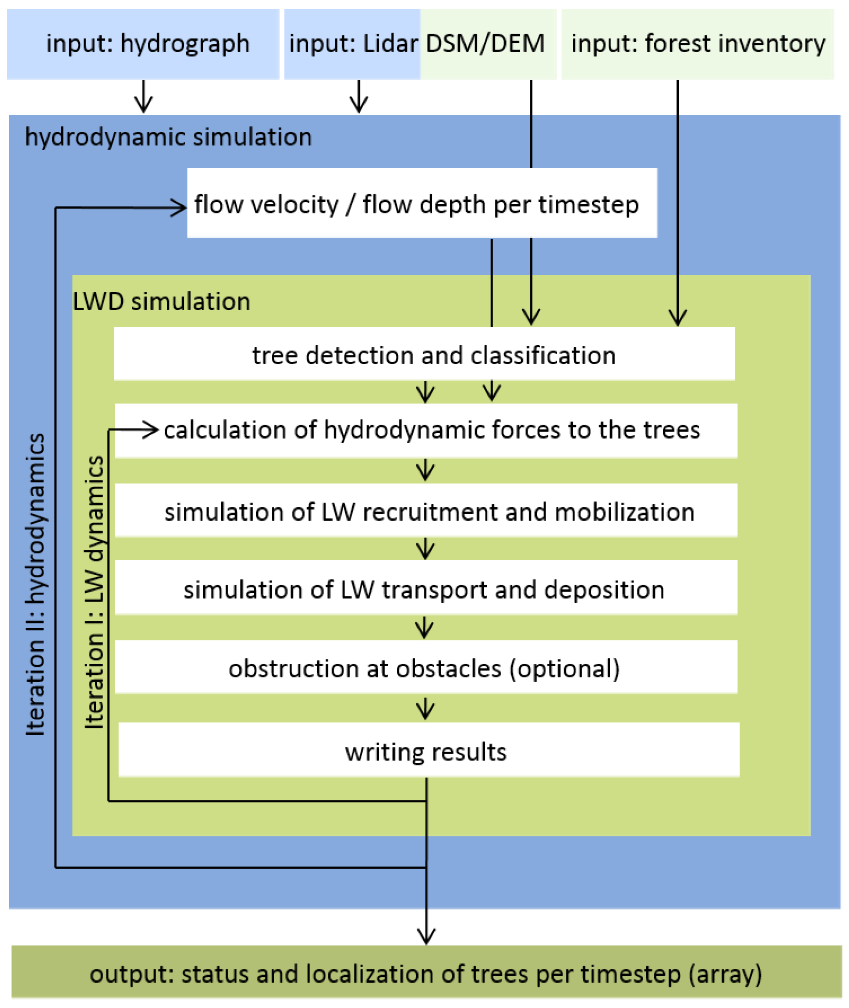
Figure 1. General framework of large wood dynamics (LWD) simulation in LWDsimR. DSM, digital surface model; DEM, digital elevation model; LW, large wood.
Water 10 01134 g001
Figure 2. Probabilities of mobilization used in the recruitment module.
Water 10 01134 g002
Figure 3. Overview of the study area. Background data: Canton of Bern.
Water 10 01134 g003
Figure 4. Simulated temporal distribution of LW dynamics in a worst case flood along the Aare River. Time step of the hydrodynamic model = 1200 s, time step of LWDsimR = 5 s.
Water 10 01134 g004
Figure 5. Extract of the map of the deposition areas in the Aare River floodplain near Rubigen. Background map: Federal Office of Topography SWISSTOPO.
Water 10 01134 g005
Figure 6. Extract of the map of the recruitment areas of LW that reached the lower system boundary at Bern during the simulation. The dots show the initial locations of the wood logs. Background map: Federal Office of Topography SWISSTOPO.
Water 10 01134 g006
Figure 7. Extract of the map of the deposition areas in the Aare River floodplain upstream of Bern. The dots show the locations of the wood logs at the end of the simulation. Background map: Federal Office of Topography SWISSTOPO.
Water 10 01134 g007
Table 1. Modelled solid LW volumes during an extreme flood in the Aare River.
LW ClassLW Volume (m3)
Forest stock in inundated areas112,661
Total mobilized wood11,841
Mobilized in Zulg tributary 343
Mobilized living wood 5732
Mobilized deadwood6109
Deposited after mobilization7288
Volume passing the lower system boundary in Bern3933