Abstract
The Soil and Water Assessment Tool (SWAT) has been calibrated in many watersheds of various sizes and physiographic features. However, it is still unclear whether SWAT calibration parameters will produce satisfactory results if they are implemented in watersheds of different sizes. Evaluating the transferability of SWAT calibration parameters between watersheds of different sizes will provide insight into whether it is acceptable to calibrate SWAT in one watershed and apply the optimized parameters in different size watersheds by assuming both watersheds have similar physiographic properties. This study investigated the influence of watershed size on the SWAT model calibration parameters transferability between four watersheds (CCW = 680 km2, F34 = 183 km2, AXL = 42 km2, and ALG = 20 km2) located in Northeastern Indiana. The results show that calibrating SWAT at one size and applying the optimized parameters at different watershed sizes of similar physiographic features provided satisfactory simulation results. The size watershed at which SWAT was calibrated had little effect on streamflow predictions. Soluble nitrogen loss estimates were improved when calibration was performed at the larger CCW watershed while calibrating SWAT at the smaller AXL and ALG watersheds produced improved statistical indicator values (NSE, R2, and PBIAS) for soluble P and total P when applied to the larger CCW and F34 watersheds.
1. Introduction
Growing concerns over water quality in agricultural watersheds continue to be the topic of many discussions. Agricultural runoff is considered a primary cause of nonpoint source pollution in the United States [1] because it often transports pesticides, nutrients, and sediment from agricultural fields and other areas to rivers and streams. This may have serious implications for the chemical, physical, and biological integrity of the nation’s water bodies [2]. The primary pollutants affecting water quality in Northeastern Indiana and much of the Midwest Corn Belt Region are nitrogen and phosphorus especially soluble phosphorus [3], which are transported in agricultural runoff.
An effective watershed management program within an agricultural watershed should minimize the loss of agricultural chemicals and maintain water quality standards [4]. Developing an effective watershed management program, however, requires comprehensive understanding of the hydrologic and chemical processes within the watershed [5]. These processes are usually examined at the watershed scale using computer simulation models such as the Soil and Water Assessment Tool (SWAT) [6]. SWAT is used to assess the effect of various management practices, and for developing and improving watershed management programs [7,8,9].
SWAT was developed for use in large ungauged watersheds and can be used to provide long-term analysis of watershed processes [10] without calibration [11]. However, SWAT model parameters vary in sensitivity during different flow regimes and for different simulation periods [12,13]. As a result, several researchers recommend that SWAT be calibrated in cases where measured data are available because calibration will improve the model’s performance and result in more accurate simulations [14,15].
Despite being calibrated in many watersheds of various sizes and physiographic features, it is still unclear whether SWAT calibration parameters will produce satisfactory results if they are implemented in watersheds of different sizes (other than the size at which they were optimized). This study evaluated SWAT model performance at the watershed outlet, with respect to performance metrics, to gain insight into whether it is acceptable to calibrate SWAT in one watershed and apply the optimized parameters in another watershed with a different size by assuming both watersheds have similar physiographic properties. Understanding the transferability of SWAT calibration parameters between watersheds is particularly important in cases where SWAT is applied in ungauged watersheds or watersheds with insufficient measured data to facilitate proper calibration/validation of the model.
Optimized parameter sets may be transferred to a neighboring watershed with similar physiographic properties such as land use, soils, and topography, which is a concept known as geographical regionalization [16]. While geographic regionalization of SWAT calibration parameters has been found to produce reasonable results [17], the effect of watershed size on parameter transferability is still uncertain. Earlier studies [18,19,20,21,22] suggested that the spatial scale had little effect on streamflow simulations but will impact nitrogen and phosphorus loss simulations. Heathman et al. [23] attempted to explore the influence of watershed size on SWAT model calibration when they compared observed versus simulated streamflow for the SWAT model calibration at the 2810 km2 St. Joseph River Basin (SJRW) in Indiana (one of the 14 Conservation Effects Assessment Project benchmark watersheds) at the 679.2 km2 Cedar Creek watershed (largest tributary in SJRW). They concluded that the watershed size at which the model was calibrated had little impact on SWAT simulated streamflow for the watersheds. This conclusion was supported by Thampi et al. [24] based on a study in the Chaliyar River Basin (Kerala, India). Srinivasan et al. [25] also calibrated SWAT in the 5157 km2 Richland and Chambers Creek watershed in the Upper Trinity Basin, Texas and validated it at the smaller Mill Creek watershed (282 km2). The researchers concluded that the model explained 84% of the variability in the observed streamflow data. Heuvelmans et al. [17] evaluated SWAT model parameter transferability between the Maarkebeek and Zwalm river basins (Belgium) and found a decline in model performance when parameters are transferred in time and space.
2. Materials and Methods
2.1. Study Area
The St. Joseph River Watershed is a 2810-km2 catchment that intersects the states of Indiana, Michigan, and Ohio (Figure 1). The headwaters of the St. Joseph River originate in Michigan and the river flows southwest through Ohio and Indiana before joining the St. Mary’s River near Ft. Wayne, Indiana to form the Maumee River. The Maumee River flows northeast into the Maumee Bay of Lake Erie in Toledo, Ohio. The Cedar Creek watershed (CCW = 679 km2) located in Northeastern Indiana (85°19′28.101″ to 84°54′12.364″ W and 41°11′47.494″ to 41°32′8.776″ N) is the largest tributary to the St. Joseph River. It intersects the counties of Allen, DeKalb, and Noble and is predominantly agricultural (68%) with approximately 15% made up of forest.
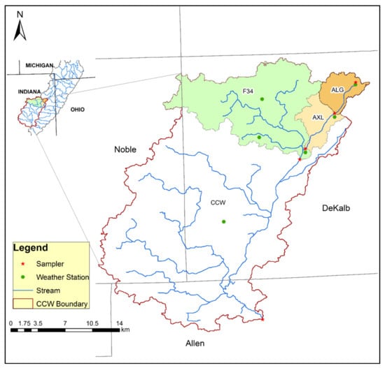
Figure 1.
Location map of the study watersheds (CCW, F34, AXL, and ALG) in Northeast Indiana with respect to the entire St. Joseph River Watershed (SJRW).
Most soils in the watersheds are comprised of the Eel-Martinsville-Genesee and Morley-Blount associations. The Eel-Martinsville-Genesee association consists of deep, moderately well-drained, nearly level, and medium-to-moderately fine-textured soils on low lands and stream terraces [5,26]. The Morley-Blount association occurs mostly in the uplands and consists of deep, moderately-to-poorly drained soils with nearly level to deep medium-textured soils [27]. Tile drainage systems drain water from many of these soils into managed drainage ditches, which alter the watershed hydrology and the transport of pesticide and nutrients across the landscape [28,29]. CCW is the largest of the four calibration watersheds analyzed in this study. The F34 (182.5 km2), AXL (41.5 km2), and ALG (19.7 km2) watersheds are nested within the upper Cedar Creek (Figure 1) and share similar physiographic features to that of Cedar Creek (Table 1).

Table 1.
Watershed characteristics including land use distribution, area, average slope, and average annual climate conditions for the study areas.
All four watersheds are located within the Clayey, High Lime Till Plains of the Eastern Corn Belt Plains (55) ecoregion. There are extensive glacial deposits of Wisconsinan age that are not as dissected nor as leached as the pre-Wisconsinan till, which is restricted to the southern part of Ecoregion 55. The Clayey, High Lime Till Plains ecoregion (55a) is transitional between the Loamy, High Lime Till Plains (55b), and the Maumee Lake Plains (57a). These soils are more artificially drained than those in Ecoregion 55b and supported fewer swampy areas than Ecoregion 57a [30]. Corn, soybean, wheat, and livestock farming is dominant and has replaced the original beech forests and scattered elm-ash swamp forests [30].
2.2. SWAT Model Description
SWAT is a lumped, semi-distributed hydrologic model developed by the USDA Agricultural Research Service (ARS) to study the effects of management decisions on water quality “with reasonable accuracy” on large ungauged watersheds [6]. SWAT requires climate inputs such as daily precipitation, maximum/minimum air temperatures, and solar radiation to simulate hydrologic processes. These climate data drive the hydrologic cycle and provide moisture and energy inputs that control the water balance. The water balance is the primary driver of the hydrologic processes, fate and transport of nutrients and pesticides, plant growth, and sediment processes in the watershed [32].
SWAT provides multiple options for estimating potential evapotranspiration (Penman-Monteith method, Priestley-Taylor or Hargreaves method) and runoff (Soil Conservation Service runoff curve number (CN) or the Green-Ampt infiltration model). The Penman-Monteith method [33] was selected for estimating evapotranspiration because it captures the effects of wind and relative humidity, which accounts for vegetation shading, wind resistance, and transpiration through leaves. This makes it suitable for application in highly vegetated watersheds. The CN method [34] was used in this study to estimate surface runoff because of its simplicity, predictability, and stability. The CN method does not require rainfall intensity and duration data. This method only requires total daily rainfall depth when estimating runoff from various land cover and soil types.
Nitrogen (N) and phosphorus (P) processes are simulated in SWAT using typical nitrogen and phosphorus cycles to track the transport and fate of various forms of N and P throughout the watershed [6]. The portion of N and P used by plants is estimated using a supply and demand approach. Nitrates, organic N, Soluble P, and organic P are removed from the soil through the mass flow of water. Nitrate loading is estimated as the product of average nitrate concentration and the volume of water present in a particular layer [6]. Soluble P loading is estimated using the solution P concentration in the top 10 mm of the soil, runoff volume, and a partitioning factor [6]. The amount of organic P transported with sediment to the stream is calculated using the Williams and Hann [35] loading function.
2.3. Model Input and Setup
The ArcSWAT version 2012.10.5a interface was used to expedite the SWAT model input and output display. To obtain suitable flow paths, the stream delineation from the National Hydrograph Dataset (NHD) was used to burn in the location of the streams in a 10-m Digital Elevation Model (DEM) obtained from USGS at a map scale of 1:24,000. The USGS National Water Quality Assessment Program (NAWQA) water quality/streamflow gauge station located near Cedarville, Allen County, Indiana was used as the watershed outlet for CCW. The USDA-ARS National Soil Erosion Research Laboratory (NSERL) water quality/streamflow gauge stations were used to specify the location of the F34, AXL, and ALG outlets. The Soil Survey Geographic Database (SSURGO) spatial data at a scale of 1:12,000 and the USDA National Agricultural Statistics Service [31] Indiana Cropland Layer were used to determine hydrologic response units (HRUs) for SWAT. All data sources are listed in Table 2.
Table 2.
Model input data.
HRUs (modeling units) are unique combinations of land use, soils, and slope classes within each subwatershed in which the model establishes management practices. SWAT first divides a watershed into smaller subwatersheds based on a specified critical source area (CSA) threshold for stream generation. CSA is a percentage of the total watershed area that determines the minimum upstream drainage area required to form a channel. Based on the assessment of CSA by Kumar and Merwade [20], a critical source area of 5% was used for each watershed in this study to achieve watershed subdivision most suited for SWAT modeling. This resulted in stream threshold areas of 30 km2, 9 km2, 2 km2, and 1 km2 for CCW, F34, AXL, and ALG, respectively (Table 3). Each subwatershed is further divided into HRUs using a specified threshold area for land use, soil types, and slope classes. The threshold for HRU definition was set to 0% land: 0% soil: 0% slope, which means we assessed all possible land use/soil/slope combinations. This facilitated spatial representation of closed depressions within the watersheds. The minimum stream threshold value and the resulting subwatersheds and HRUs for each of the study watersheds are shown in Table 3.
Table 3.
Minimum stream threshold values and the resulting subwatersheds and HRUs for each of the study watersheds.
Climate data including precipitation, maximum and minimum air temperatures, solar radiation, relative humidity, and wind speed were obtained from 10 CEAP weather stations located in the upper Cedar Creek region from 2003 to 2013. Daily precipitation and maximum and minimum air temperatures were also available from the National Climate Data Center [39] for the Auburn, Angola, Butler, Garrett, and Waterloo stations located within or around the watershed with records from 1980 to 2013. Missing data for a given station were estimated by averaging values for the nearest weather stations typically within a 5-km radius.
Area-specific land management data were collected by the ARS-NSERL through the CEAP program as well as from the DeKalb and Allen Counties Soil and Water Conservation Districts (SWCDs) and were used to represent the current management practices occurring in the watersheds. Conservation tillage has been widely adopted in the watersheds. In DeKalb County, 34% of all corn and 77% of all soybeans planted in 2012 were under a no-till system or mulch-till system. Therefore, no-till and conventional tillage were used as input in the SWAT management files, which were constructed to simulate corn/soybeans (the predominant crops in the watersheds) and rotated on all lands classified as corn or soybeans. All lands classified as wheat were simulated in a three-year rotation with corn and soybeans (corn/soybeans/wheat). The management scheme includes yearly tillage operations, nutrient and pesticide application rates, and planting and harvesting dates (Table 4 and Table 5).
Table 4.
Management operations for land in corn/soybeans rotation.
Table 5.
Management operations for land in winter wheat production (following corn/soybeans rotation in Table 4).
Tile drainage was assumed for all corn, soybean, and winter wheat areas. Tile drainage was considered to have an average depth of 1.0 m, 48 h of drainage after a rain to reach field capacity, and a drain tile lag time of 24 h [5,40]. The spacing between tiles (estimated based on soil type and drainage) is 20 m.
Closed depressions (potholes) and tile inlets were also addressed in the SWAT configurations. To represent potholes in SWAT, ArcGIS was used to process a 1-m DEM of the entire study area. This involved: (1) identifying sink features in the elevation dataset, (2) classifying sink features as potholes based on certain criteria [41], (3) creating pothole look-up tables that linked pothole features with SWAT HRUs, and (4) updating SWAT HRU files using a simple Python script. Percentages of watershed areas contributing flow to farmed closed depressions were estimated at 5.1%, 8.2%, 10.0%, and 8.7% for CCW, F34, AXL, and ALG, respectively. Average depths of potholes were 0.94 m, 0.82 m, 0.91 m, and 0.90 m for CCW, F34, AXL, and ALG, respectively.
SWAT was set up to run on a daily time step for the period between 2001 to 2013 with a warm-up period of five years (01/2001 to 12/2005). The warm-up period is recommended for the model to initialize and approach reasonable starting values for model variables [42] before beginning the calibration process.
2.4. Model Calibration and Validation
Calibration is the process used to optimize parameters in a model using observed conditions to reduce prediction uncertainty. Parameters in SWAT were calibrated at the monthly time scale in a distributed fashion using the SWAT-CUP autocalibration tool. Calibration was performed at the F34, AXL and ALG outlets for streamflow, NO3− + NO2− nitrogen (soluble N), total nitrogen (total N), orthophosphate (soluble P), and total phosphorus (total P) over a 4-year period (01/2006 to 12/2009). Due to limited data availability, SWAT could only be calibrated at the CCW outlet near Cedarville for streamflow (01/2006 to 12/2009), soluble N (04/2006 to 12/2009), and total P (4/2006 to 2009).
Historical measured data for streamflow, soluble N and total P concentrations were obtained from the St. Joseph River Watershed Initiative for the CCW outlet near Cedarville while soluble N, total N, soluble P, and total P concentrations were obtained from the ARS-NSERL-CEAP database for the F34, AXL, and ALG outlets. Measured data for total nitrogen and total phosphorus were also obtained from the ARS-NSERL-CEAP database for the F34, AXL, and ALG outlets. Concentration values for nutrients obtained from ARS were multiplied by flow on a daily time step to obtain total daily loads. Since the end goal of SWAT simulations was to evaluate long-term average annual loads, the daily loads were further aggregated into total monthly loads, which were used to perform monthly calibration and validation of the F34, AXL, and ALG SWAT configurations. The nutrient data obtained from the SJRWI were biweekly grab samples (not sufficient to perform monthly calibration). Therefore, the Load Estimator (LOADEST) was used to estimate monthly constituent loads for CCW. LOADEST [43] requires a time series of streamflow and available constituent data to develop a regression model for estimating the constituent load. A summary of the average measured streamflow and nutrient loads from each watershed for 2006 through 2013 is presented in Table 6.
Table 6.
Annual streamflow rates and nutrient loads measured from each watershed for 2006–2013.
The measured streamflow data from USGS and the ARS-NSERL-CEAP project are comprised of the baseflow and surface runoff. Baseflow is the groundwater contribution to streamflow, which needs to be separated so that measured surface flow can be compared to simulated values [5]. The Web-based Hydrograph Analysis Tool (WHAT) developed by Purdue University [44] based on the Arnold and Allen [45] baseflow filter program was used to separate storm flow from the baseflow. Optimization of the SWAT configurations ensured that simulated baseflow was approximately the fraction of water yield contributed by the baseflow from the measured flow estimated by WHAT.
After calibration, the next step was to validate the model performance and ensure it can perform simulations correctly and is suitable for use in decision-making. Validation was performed for F34, AXL, and ALG configurations over a 4-year period (01/2010 to 12/2013). The CCW configuration was validated for streamflow over a 4-year period (01/2010 to 12/2013) and soluble N and total P over a 3-year period (01/2010 to 12/2012) due to limited data availability.
To evaluate the effects of watershed size on SWAT model calibration, the optimized parameters for each SWAT configuration (CCW, F34, AXL, and ALG) were applied to subsequent configurations. For example, parameters optimized at the CCW level during the calibration process were later implemented at the F34, AXL, and ALG levels and their effect on streamflow, nitrogen, and phosphorus loss were evaluated.
2.5. SWAT-CUP Calibration with SUFI-2
The calibration and uncertainty programs for SWAT (SWAT-CUP) developed by Abbaspour et al. [46] were used to aid in the calibration process. The SUFI-2 algorithm was selected in SWAT-CUP to optimize nine parameters for monthly streamflow volume and 10 parameters were directly related to sediment, nitrogen, and phosphorus losses (Table 7). The selection of optimization parameters and parameter ranges were based on an extensive literature review [5,11,13,20,32,47,48] and an earlier sensitivity analysis that was performed for CCW [49]. SUFI-2 was selected because it required less iterations to achieve optimization and it accounted for model uncertainty as well as uncertainty associated with model parameters and measured variables (e.g., discharge) [50]. The Kling–Gupta efficiency (KGE) [51] was used as the objective function for optimizing SWAT input parameters (1).
where r is the linear correlation coefficient between corresponding simulated and observed values, is a measure of relative variability in the simulated and observed values, and is the bias between the mean simulated and mean observed data. Steps involved in setting up and executing the SWAT-CUP are outlined in Reference [50].
Table 7.
List of SWAT parameters used for calibration of CCW, F34, AXL, and ALG configurations.
2.6. Evaluating Model Performance
In addition to visual inspection of observed and simulated time series values at the watershed outlets, model performance was also evaluated using KGE, the coefficient of determination (R2) (2), the Nash-Sutcliffe efficiency (NSE; [52]) (3), and percent bias () (4). The R2 value is an indicator of the strength of the linear relationship between the observed and simulated values. The NSE simulation coefficient indicates how well the plot of observed versus simulated values fits the 1:1 line and it can range from −∞ to +1 with +1 being in perfect agreement between the model and observed data [15]. Both R2 and NSE are sensitive to high flows and, therefore, was used to measure the average tendency of the simulated data to be larger or smaller than the measured data. The optimum value is zero and low magnitude values indicate better simulations. Positive values indicate model underestimation and negative values indicate model overestimation. The equations are shown below.
where is the average measured value during the simulation period, is the average of the simulated values during the simulation period, is the measured data on day i, is the simulated output on day i, and j represents the rank.
Based on model evaluation performance-ratings adopted from References [53,54], streamflow simulations were considered reasonable if NSE > 0.50, R2 > 0.50 and was within ±25% while nitrogen and phosphorus loss simulations were considered reasonable if NSE > 0.36, R2 > 0.50, and was within ±70%.
3. Results
All four watersheds were calibrated for the period between January 2006 to December 2009 and validated for the period between January 2010 to December 2013. SWAT calibration and validation results of monthly streamflow, soluble N, total N, soluble P, and total P are presented in Table 8, Table 9, Table 10, Table 11 and Table 12 for all watershed configurations.
Table 8.
Streamflow calibration and validation statistical metrics for CCW, F34, AXL, and ALG SWAT model performance.
Table 9.
Soluble N load calibration and validation statistical metrics for CCW, F34, AXL, and ALG SWAT model performance.
Table 10.
Total N load calibration and validation statistical metrics for SWAT model performance for CCW, F34, AXL, and ALG.
Table 11.
Soluble P load calibration and validation statistical metrics for SWAT performance for CCW, F34, AXL, and ALG.
Table 12.
Total P load calibration and validation statistical metrics for CCW, F34, AXL, and ALG SWAT model performance.
3.1. Streamflow Calibration and Validation
SWAT was successfully calibrated for monthly streamflow at the outlets of four watersheds located in Northeastern Indiana (Figure 2a–d). For the calibration period, WHAT estimated that 58%, 61%, 56%, and 59% of measured streamflow at the outlets of CCW, F34, AXL, and ALG, respectively, was the baseflow. In comparison, the SWAT model estimated 52%, 53%, 51%, and 51% as baseflow at the respective watershed outlets. The long-term water balance simulated by the model was similar to the water balance simulated for CCW in prior studies [5,20]. Therefore, the long-term water balances simulated by SWAT were considered to generate acceptable predictions representative of the study areas. Summary values with comparable units of the main magnitudes of the hydrological balance (precipitation, evapotranspiration, runoff, infiltration, drainage, etc.) are presented in Table A1 and Table A2, respectively, of the Appendix.
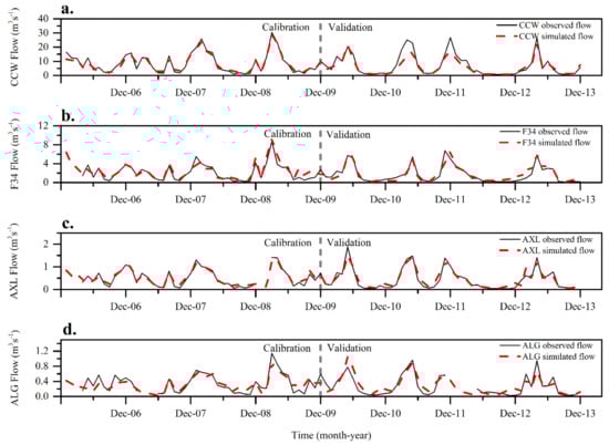
Figure 2.
Monthly time series of simulated and observed streamflow for (a) CCW, (b) F34, (c) AXL, and (d) ALG. Calibration period was from January 2006 to December 2009 and the validation period was from January 2010 to December 2013.
Measured monthly streamflow data for the Cedar Creek watershed (USGS Gauge #04180000) and the ARS CEAP study watersheds (F34, AXL, and ALG outlets) were compared with monthly SWAT simulated streamflow for the calibration period. Plots of simulated versus observed monthly streamflow at the different calibration scales are presented in Figure 3a–d. As depicted in Figure 3, SWAT could predict monthly streamflow in a satisfactory way at all four watershed sizes with most of the data points falling along the 1:1 line. Regression lines drawn through the data points indicated that streamflow was best predicted at the CCW, F34, and AXL outlets but slightly underestimated at the ALG outlet (the smallest of the watersheds). In general, modeled streamflow at the respective watershed outlets produced similar results despite the size of the watershed at which the model was calibrated (Figure 3).
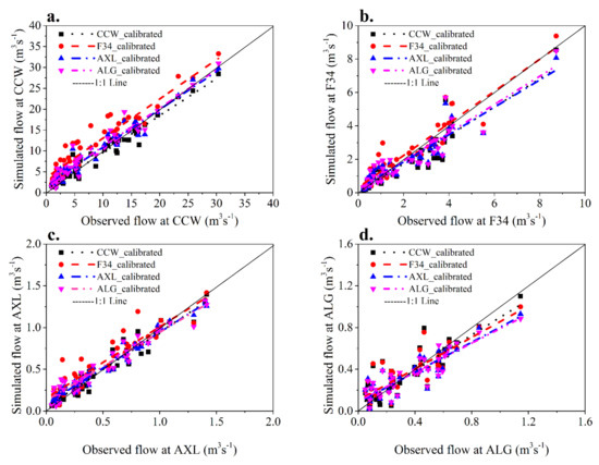
Figure 3.
One-to-one plots of SWAT simulated vs. observed monthly streamflow at the (a) CCW outlet, (b) F34 outlet, (c) AXL outlet, and (d) ALG outlet for the calibration period from January 2006 to December 2009.
A summary of the statistical analyses of monthly streamflow for calibration and validation are presented in Table 8. Before calibration, there were acceptable KGE, NSE, R2, and PBIAS values for SWAT simulations at all four watersheds (NSE > 0.50, R2 > 0.50 and ± 25%)). However, calibration improved the performance metrics especially in terms of KGE and PBIAS.
3.2. Nitrogen Calibration and Validation
Measured monthly nitrogen loads in the form of nitrate+nitrite (referred to as soluble N) and total nitrogen (referred to as total N) for the Cedar Creek watershed (USGS Gauge #04180000) and the ARS CEAP study watersheds (F34, AXL, and ALG outlets) were compared with SWAT simulated monthly soluble N and total N loads (Figure A1 and Figure A2, respectively, in Appendix A). Results showed that SWAT was successfully calibrated at all four watershed scales for monthly soluble N load and at F34, AXL, and ALG for monthly total N load. No data were available for total N at the CCW scale and soluble N data at CCW were only available from 2008 to 2013. Performance evaluation metrics for calibration, validation, and non-calibrated model results for soluble N and total N are presented in Table 9 and Table 10, respectively. SWAT could predict monthly soluble N and total N loads well at the different watershed sizes. Most of the data points for soluble N predictions occurred close to the 1:1 line, which is depicted by the plots of simulated versus observed monthly soluble N loads at the different watershed sizes presented in Figure 4a–d.
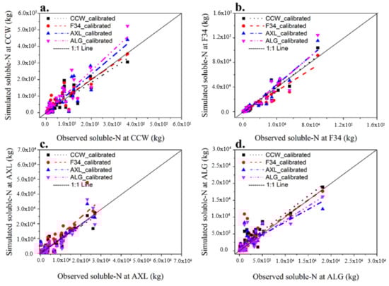
Figure 4.
One-to-one plots of SWAT simulated vs. observed monthly soluble N loads at the (a) CCW outlet, (b) F34 outlet, (c) AXL outlet, and (d) ALG outlet for the calibration period from January 2006 to December 2009.
For soluble N loads, when SWAT was calibrated for CCW, the NSE, R2, and PBIAS values were all within acceptable ranges when its optimized parameter values were used in F34, AXL, and ALG watershed simulations (Table 9). During the validation period, all four watersheds also produced acceptable KGE, NSE, R2, and PBIAS values. Despite R2 values above 0.50 and PBIAS lower than 70%, when SWAT was calibrated at the F34 scale and its optimized parameters implemented at the CCW, AXL and ALG watershed scales, both the KGE and NSE values were outside the acceptable limits in the CCW, AXL, and ALG simulations. During the validation period, only F34 and ALG produced acceptable results. When SWAT was calibrated at the AXL watershed outlet and its optimized parameters implemented at the CCW, F34 and ALG watersheds sizes, NSE, R2, and PBIAS values were all within acceptable ranges. During the validation period, all four-watershed simulations also produced acceptable KGE, NSE, R2, and PBIAS values. When calibration was performed at the ALG watershed outlet and the optimized parameters implemented at the CCW, F34, and AXL watershed sizes, NSE, R2, and PBIAS values were also all within the acceptable ranges. During the validation period, all four-watershed simulations produced acceptable statistical values.
For total N loads, despite reasonable R2 values and a PBIAS of 59.4 at the ALG outlet, when SWAT was calibrated at the F34 watershed outlet and its optimized parameters were used in AXL and ALG watershed simulations, the resulting model performance was unsatisfactory. KGE and NSE values were below the acceptable limits for the AXL and ALG simulations (Table 10). During the validation period, both F34 and ALG produced acceptable results while AXL produced unsatisfactory KGE, NSE, and results. When SWAT was calibrated at the AXL and ALG watershed outlets and the optimized parameters were used in the respective watershed simulations, the NSE, R2, and PBIAS values were all within the acceptable range. During the validation period, all four-watershed simulations also produced acceptable statistical values (Table 10).
3.3. Phosphorus Calibration and Validation
Measured monthly phosphorus loads in the form of orthophosphate (referred to as soluble P) and total phosphorus (referred to as total P) for the Cedar Creek watershed (USGS Gauge #04180000) and the ARS CEAP study watersheds (F34, AXL, and ALG outlets) were compared with SWAT simulated monthly soluble P and total P loads (Figure A3 and Figure A4, respectively, in Appendix A). Results indicated that SWAT was successfully calibrated at F34, AXL, and ALG for monthly soluble P loads at all four watersheds for monthly total P loads from January 2006 to December 2009. They were also validated between January 2010 to December 2013. No data were available for soluble P nor for CCW. A summary of the performance evaluation metrics for calibration, validation, and non-calibrated model results for monthly soluble P and total P loads are presented in Table 11 and Table 12, respectively. In this case, SWAT predicted monthly soluble P and total P loads well with most of the data points occurring close to the 1:1 line, which is depicted by the plots of simulated versus observed monthly soluble P loads at the different watershed sizes (see Figure 5).
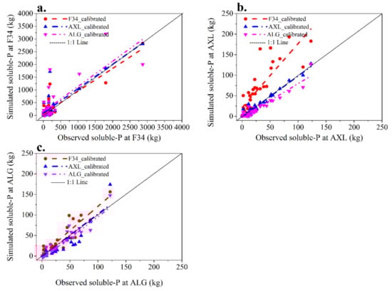
Figure 5.
One-to-one plots of SWAT simulated vs. observed monthly soluble P loads at the (a) F34 watershed outlet, (b) AXL watershed outlet, and (c) ALG watershed outlet for the calibration period from January 2006 to December 2009.
Modeled soluble P loads at the F34 (Figure 5a), AXL (Figure 5b), and ALG (Figure 5c) watershed outlets produced similar results despite the watershed size at which the model was calibrated, with a few exceptions. When calibration was performed at the F34 watershed outlet and its optimized parameters were applied to the AXL watershed, the KGE, NSE, and PBIAS values were outside the acceptable ranges (Table 11). However, when the F34-optimized parameters were applied in the ALG watershed simulations, they produced satisfactory results. During the validation period, only F34 and ALG produced acceptable results.
When calibration was performed at the AXL watershed outlet, NSE, R2, and PBIAS values for predicting monthly soluble P losses were all satisfactory at F34 and ALG. Model results were also within a satisfactory range during the validation period for all three-watershed simulations.
When calibration was performed at the ALG watershed and the optimized parameters were applied in the F34 and AXL watershed simulations, the performance metrics were unsatisfactory at F34 with KGE = 0.35 and NSE = 0.31. However, during the validation period, all three-watershed simulations produced acceptable statistical values.
Modeled total P losses at the CCW, F34, AXL, and ALG watershed outlets produced similar results despite the scale at which the model was calibrated, with only a few exceptions (Table 12). When SWAT was calibrated at the CCW outlet, the NSE, R2, and PBIAS values for total P loss predictions were all within the acceptable ranges when its optimized parameter values were applied to the four watershed simulations. During the validation period, the NSE, R2, and PBIAS values were also all acceptable. When SWAT was calibrated at the F34 watershed outlet and its optimized parameters were applied in the CCW, AXL, and ALG watershed simulations, the resulting model performance was acceptable except at AXL where KGE = 0.35. During the validation period, all four watersheds produced results within the acceptable ranges. When calibration was performed at the AXL watershed outlet and at the ALG watershed outlet, the KGE, NSE, R2, and PBIAS values were all within the acceptable range for CCW, F34, AXL, and ALG watershed simulations. During the validation period, all four watershed scales produced satisfactory statistical values.
4. Discussion
In terms of the effects of watershed size on SWAT model calibration for streamflow, nitrogen loads and phosphorus loads were evaluated at four watersheds: Cedar Creek watershed (CCW) located in Northeastern Indiana, F34 (approximately 27% of CCW), AXL (approximately 6% of CCW), and ALG (approximately 3% of CCW). Based on the results presented in this paper, SWAT satisfactorily simulated streamflow, soluble N, total N, soluble P, and total P at the four watershed scales with slight differences between the scales at which the calibrations were performed.
Model efficiency evaluations indicated that streamflow calibration at the smaller AXL and ALG watershed sizes produced similar KGE, NSE, R2, and PBIAS values when compared to calibrations performed at the larger watershed sizes. While there are very few studies examining the effects of the calibration scale on SWAT model performance, these results agree with findings from previous studies [23,24]. Notable similarities in both studies include the fact that the study watersheds were nested within each other and had similar physiographic features (such as slope, land use distribution, and soil type) that may have resulted in similar parameterization of the model. Because the CN method is not very sensitive to the size of the watershed, the impact of surface runoff contributions to streamflow was not influenced significantly by the watershed size [19].
In terms of nitrogen and phosphorus load simulations, calibration had a large impact on SWAT model predictions. Despite significantly improved results at all watershed sizes due to calibration, when SWAT was calibrated at the larger CCW watershed, its optimized parameters produced improved soluble N and total P simulations when applied at the smaller watershed sizes. Optimizing SWAT parameters for the AXL watershed resulted in improved predictions of soluble N and total N losses when applied at the smaller ALG watershed. This was due to the closeness in their average slope, land use distribution, management practices, and other physiographic properties that resulted in similar values for the calibration parameters. Similarly, calibrating SWAT at the smaller ALG and AXL watersheds produced improved NSE, R2, and PBIAS values for soluble P and total P loads when applied to the larger watersheds. The calibrated parameters for CCW, AXL, and ALG were similar in terms of final values (or percent change) and the level of sensitivity (Table 8), which was the underlying reason for the different watershed configurations producing satisfactory results regardless of the optimization scale.
In general, SWAT predictions at the respective watershed outlets produced similar results despite the scale at which the model was calibrated with one notable exception. Although calibration at the F34 outlet was satisfactory for each constituent, when the optimized F34 parameters were applied to the other watershed configurations, the results were not always satisfactory. This was most likely due to inconsistencies in the F34 observed dataset used for SWAT calibrations. F34 had a larger proportion of high flow events compared to the other three watersheds and, because nitrogen and phosphorus loads were calculated as a function of streamflow, they too were affected by any adjustments made during the calibration process. During autocalibration, SWAT parameters were adjusted to accommodate the higher events, which then overestimated the various processes when applied to the different watershed configurations. These results indicate greater uncertainty in SWAT calibrations for F34, which may be due to the characteristics of farmed closed depressions (potholes) within F34 when compared to the other watersheds. The average depth of farmed closed depressions in F34 was smaller than that of CCW, AXL, and ALG, which would affect the maximum volume of ponded water in the watershed. The inclusion of potholes adds to the complexities of SWAT and the model calibration process. Consequently, optimizing SWAT model parameters for F34 often resulted in over-prediction of the streamflow and nitrogen and phosphorus losses when applied to the CCW, AXL, and ALG watersheds.
Nitrogen and phosphorus loads calculated for the F34 outlet were affected by the observed flow data, which indirectly influenced the calibration parameters. This was evident in the parameter sensitivity rankings (Table 7) where the most sensitive nitrogen and phosphorus parameters for F34 were the nitrogen uptake distribution factor (N_UPDIS) and the phosphorus soil-partition coefficient (PHOSKD), respectively. While the most sensitive parameters for CCW were the nitrogen percolation coefficient (NPERCO) and the phosphorus uptake distribution (P_UPDIS), for both the AXL and ALG watersheds, the most sensitive parameters were the Denitrification exponential rate constant (CDN) and P_UPDIS. These differences in sensitivity between F34 and the other watersheds means that small changes in a non-sensitive parameter for F34 may result in big differences when applied to other watersheds. For example, the least sensitive parameter in the simulation of nitrogen loads for F34 was humus mineralization of active organic nitrogen (CMN), which was the second most sensitive for AXL and ALG. The final calibrated CMN value for F34 was twice that of AXL and ALG, which means that, when applying the F34 CMN to AXL and ALG, it would result in more nitrogen mineralization and over-prediction of soluble N losses.
Additionally, a major disadvantage with NSE and R2 evaluations is that the differences between observed and simulated data are calculated as squared values, which makes them biased towards high flows. As a result, larger values in the calibration time series strongly influenced the calibration outcome while lower values were neglected [55]. As seen in Figure 3, Figure 4 and Figure 5, there were more occurrences of higher monthly values in the F34 dataset above the 1:1 line, which could explain the poor statistics for nitrogen calibration for F34 despite satisfactory results over the calibration period. The nutrient load predictions might have been improved had there been sufficient sediment data available to improve model calibration.
5. Conclusions
There are several issues to consider in the application of watershed scale hydrologic modeling, including the influence of watershed size on model calibration parameters. This is especially true when using the model as an environmental assessment tool or as a decision-support system for soil and water resource management. This study sought to answer the question: how does watershed size affect the transferability of SWAT calibration parameters for the simulation of streamflow as well as nitrogen and phosphorus loss in agricultural watersheds with similar physiographic properties?
Based on the results presented in this paper, calibrating SWAT at one watershed size and applying the optimized parameters at different sizes may produce satisfactory results despite a drop in the model performance when parameters are transferred across watersheds. These results are possible in SWAT model simulations because the study watersheds were nested within each other and had similar physiographic features that resulted in similar parameterization. However, as shown in the optimization performed at F34, when SWAT parameters vary in sensitivity between watersheds, they are likely to produce lower KGE and NSE values at different watershed sizes.
Based on the results of this study and the constraint of similar physiographic properties, the size of the watershed for which SWAT is calibrated tends to have a greater impact on nitrogen and phosphorus loss simulations than on streamflow predictions. Calibrating SWAT at the smaller watershed sizes was successful in reducing the bias between measured data and SWAT simulations while maintaining model efficiency. In some instances, the goodness-of-fit measures used to evaluate model efficiency were improved when the model was calibrated at the smaller ALG (20 km2) watershed and then applied at the larger CCW (679 km2) watershed.
This study has demonstrated that, with proper calibration of SWAT, it is possible to transfer optimized parameters from one watershed size to another. However, more research is needed to determine under what condition (or sets of conditions) this will be applicable. Additionally, more in-depth research is needed to understand the influence of watershed sizes on SWAT calibration parameters across different ecoregions and for land use/land cover changes.
Author Contributions
C.W.W. was responsible for the study conceptualization. C.W.W. and D.C.F. managed the data curation. C.W.W. handled the formal analysis and project methodology. C.W.W. and D.C.F. took part in the investigation. D.C.F. and B.A.E. were responsible for managing resources. D.C.F. and B.A.E. supervised the project. B.A.E. was responsible for validating the findings. C.W.W. took part in visualization and wrote the original draft. D.C.F. and B.A.E. were responsible for reviewing and editing the manuscript.
Conflicts of Interest
The authors declare no conflict of interest. Mention of company or trade names is for description only and does not imply endorsement by the USDA. The USDA is an equal opportunity provider and employer.
Appendix A
Calibration/Validation plots for soluble N, soluble P, total N, and total P. Calibration period was from January 2006 to December 2009 and the validation period was from January 2010 to December 2013.

Figure A1.
Monthly time series of simulated and observed soluble N for the calibration/validation period. (a) CCW, (b) F34, (c) AXL, and (d) ALG.

Figure A2.
Monthly time series of simulated and observed total N for (a) F34, (b) AXL, and (c) ALG. There were no measured total N data available for CCW to perform calibration and validation.

Figure A3.
Monthly time series of simulated and observed soluble P for (a) F34, (b) AXL, and (c) ALG. There were no measured soluble P data available for CCW to perform calibration and validation.

Figure A4.
Monthly time series of simulated and observed total P for (a) CCW, (b) F34, (c) AXL, and (d) ALG.
Table A1.
Average annual hydrologic balance for CCW, F34, AXL, and ALG watersheds.
Table A1.
Average annual hydrologic balance for CCW, F34, AXL, and ALG watersheds.
| Hydrologic Parameters | CCW (mm) | F34 (mm) | AXL (mm) | ALG (mm) |
|---|---|---|---|---|
| Precipitation | 982.7 | 982.7 | 982.7 | 982.7 |
| Snow Fall | 98.53 | 99.37 | 98.61 | 98.60 |
| Snow Melt | 97.88 | 98.65 | 97.82 | 97.82 |
| Sublimation | 0.00 | 0.01 | 0.00 | 0.00 |
| Surface Runoff Flow | 166.58 | 148.27 | 163.47 | 168.01 |
| Lateral Soil Flow | 21.13 | 8.92 | 9.68 | 9.66 |
| Tile Flow | 19.40 | 8.63 | 9.33 | 8.89 |
| Groundwater (SHAL AQ) Flow | 177.88 | 197.90 | 225.65 | 217.83 |
| Groundwater (DEEP AQ) Flow | 0.00 | 0.00 | 0.00 | 0.00 |
| Deep AQ Recharge | 38.61 | 34.67 | 1.72 | 1.67 |
| Total AQ Recharge | 218.52 | 234.42 | 229.24 | 222.17 |
| Total Water YLD | 385.10 | 363.89 | 408.28 | 404.54 |
| Percolation out of Soil | 218.99 | 233.81 | 228.86 | 221.76 |
| ET | 557.8 | 585.9 | 572.8 | 575.7 |
| PET | 817.6 | 817.5 | 813.5 | 813.5 |
Table A2.
Average annual nutrients balance for CCW, F34, AXL, and ALG watersheds.
Table A2.
Average annual nutrients balance for CCW, F34, AXL, and ALG watersheds.
| Nutrients Parameters | CCW (kg/ha) | F34 (kg/ha) | AXL (kg/ha) | ALG (kg/ha) |
|---|---|---|---|---|
| Organic N | 11.231 | 10.456 | 11.176 | 11.575 |
| Organic P | 1.445 | 1.364 | 1.461 | 1.515 |
| NO3 Yield (Surface Flow) | 0.743 | 2.592 | 2.315 | 1.883 |
| NO3 Yield (LAT) | 0.351 | 0.265 | 0.21 | 0.202 |
| NO3 Yield (TILE) | 2.478 | 3.031 | 1.807 | 1.797 |
| SOLP Yield (TILE) | 0.074 | 0.052 | 0.045 | 0.052 |
| SOL P Yield | 0.065 | 0.126 | 0.103 | 0.119 |
| NO3 Leached | 14.061 | 45.058 | 22.311 | 22.059 |
| P Leached | 0.091 | 0.097 | 0.095 | 0.092 |
| N Uptake | 145.345 | 185.108 | 165.347 | 164.242 |
| P Uptake | 24.774 | 31.632 | 28.161 | 27.94 |
| NO3 Yield (Ground Water Flow) | 0.521 | 2.264 | 1.042 | 1.002 |
| Active to Solution P Flow | 4.028 | 1.437 | 1.971 | 1.436 |
| Active to STABLE P Flow | 3.49 | 1.191 | 1.707 | 1.245 |
| N Fertilizer Applied | 42.47 | 36.406 | 40.128 | 38.975 |
| P Fertilizer Applied | 11.335 | 11.335 | 11.335 | 11.199 |
| N Fixation | 91.153 | 87.209 | 99.911 | 98.864 |
| Denitrification | 74.212 | 8.776 | 55.434 | 51.257 |
| Humus Mineral on Active Organic N | 36.133 | 37.882 | 34.755 | 31.757 |
| Humus Mineral on Active Organic P | 6.211 | 6.522 | 5.996 | 5.48 |
| Mineral from Fresh Organic N | 74.784 | 100.079 | 82.817 | 82.187 |
| Mineral from Fresh Organic P | 15.055 | 19.938 | 16.901 | 16.759 |
| NO3 in Rainfall | 9.457 | 8.676 | 9.379 | 9.38 |
| Initial NO3 in Soil | 68.926 | 68.926 | 68.926 | 68.926 |
| Final NO3 in Soil | 11.386 | 58.248 | 23.709 | 24.496 |
| Initial Organic N in Soil | 12,462.135 | 12,462.135 | 12,462.135 | 12,462.135 |
| Final Organic N in Soil | 12,159.925 | 12,261.58 | 12,228.893 | 12,268.814 |
| Initial Mineral P in Soil | 4037.205 | 4037.205 | 4037.205 | 4037.205 |
| Final Mineral P in Soil | 4099.935 | 4053.268 | 4070.857 | 4061.598 |
| Initial Organic P in Soil | 1526.612 | 1526.612 | 1526.612 | 1526.612 |
| Final Organic P in Soil | 1486.104 | 1504.575 | 1499.159 | 1506.023 |
| NO3 in Fertilizer | 42.323 | 36.258 | 39.98 | 38.825 |
| Ammonia in Fertilizer | 0.148 | 0.148 | 0.148 | 0.151 |
| Organic N in Fertilizer | 0 | 0 | 0 | 0 |
| Mineral P in Fertilizer | 11.335 | 11.335 | 11.335 | 11.199 |
| Organic P in Fertilizer | 0 | 0 | 0 | 0 |
| N removed in Yield | 61.491 | 79.163 | 72.643 | 72.354 |
| P removed in Yield | 8.378 | 10.621 | 9.836 | 9.788 |
| Ammonia Volatilization | 0.007 | 0.007 | 0.007 | 0.007 |
| Ammonia Nitrification | 0.141 | 0.141 | 0.141 | 0.144 |
References
- Yu, C.-Y.; Northcott, W.J.; McIsaac, G. Development of an artificial neural network model for hydrologic and water quality modeling of agricultural watersheds. Trans. ASAE 2004, 47, 285–290. [Google Scholar] [CrossRef]
- United States Environmental Protection Agency (USEPA). National Water Quality Inventory: 1992 Report to Congress; EPA-841-R-94-001; USEPA: Washington, DC, USA, 1994. [Google Scholar]
- Charlton, M.; Vincent, J.; Marvin, C.; Ciborowski, J. Status of Nutrients in the Lake Erie Basin; US EPA; Great Lakes National Program Office: Chicago, IL, USA, 2008; pp. 1–42. [Google Scholar]
- Tripathi, M.; Panda, R.; Raghuwanshi, N. Development of effective management plan for critical subwatersheds using SWAT model. Hydrol. Process. 2005, 19, 809–826. [Google Scholar] [CrossRef]
- Larose, M.; Heathman, G.C.; Norton, L.D.; Engel, B. Hydrologic and atrazine simulation of the Cedar Creek watershed using the SWAT model. J. Environ. Qual. 2007, 36, 521–531. [Google Scholar] [CrossRef] [PubMed]
- Arnold, J.G.; Srinivasan, R.; Muttiah, R.S.; Williams, J.R. Large area hydrologic modeling and assessment part I: Model development. J. Am. Water Resour. Assoc. 1998, 34, 73–89. [Google Scholar] [CrossRef]
- Spruill, C.; Workman, S.; Taraba, J. Simulation of daily and monthly stream discharge from small watersheds using the SWAT model. Trans. ASAE 2000, 43, 1431. [Google Scholar] [CrossRef]
- Wallace, C.W.; Flanagan, D.C.; Engel, B.A. Quantifying the effects of conservation practice implementation on predicted runoff and chemical losses under climate change. Agric. Water Manag. 2017, 186, 51–65. [Google Scholar] [CrossRef]
- Wallace, C.W.; Flanagan, D.C.; Engel, B.A. Quantifying the Effects of Future Climate Conditions on Runoff, Sediment, and Chemical Losses at Different Watershed Sizes. Trans. ASABE 2017, 60, 915–929. [Google Scholar] [CrossRef]
- Borah, D.K.; Arnold, J.G.; Bera, M.; Krug, E.C.; Liang, X.-Z. Storm event and continuous hydrologic modeling for comprehensive and efficient watershed simulations. J. Hydrol. Eng. 2007, 12, 605–616. [Google Scholar] [CrossRef]
- Neitsch, S.; Arnold, J.; Kiniry, J.; Srinivasan, R.; Williams, J. Soil and Water Assessment Tool User’s Manual Version 2000. GSWRL Report 02-02. 2002. p. 202. Available online: https://swat.tamu.edu/media/1294/swatuserman.pdf (accessed on 1 June 2018).
- Kannan, N.; White, S.; Worrall, F.; Whelan, M. Sensitivity analysis and identification of the best evapotranspiration and runoff options for hydrological modelling in SWAT-2000. J. Hydrol. 2007, 332, 456–466. [Google Scholar] [CrossRef]
- White, K.L.; Chaubey, I. Sensitivity analysis, calibration, and validations for a multisite and multivariable SWAT model. J. Am. Water Resour. Assoc. 2005, 41, 1077–1089. [Google Scholar] [CrossRef]
- Kirsch, K.; Kirsch, A.; Arnold, J. Predicting sediment and phosphorus loads in the Rock River basin using SWAT. Trans. ASAE 2002, 45, 1757. [Google Scholar] [CrossRef]
- Santhi, C.; Arnold, J.G.; Williams, J.R.; Dugas, W.A.; Srinivasan, R.; Hauck, L.M. Validation of the SWAT model on a large river basin with point and nonpoint sources. J. Am. Water Resour. Assoc. 2001, 37, 1169–1188. [Google Scholar] [CrossRef]
- Vandewiele, G.; Elias, A. Monthly water balance of ungauged catchments obtained by geographical regionalization. J. Hydrol. 1995, 170, 277–291. [Google Scholar] [CrossRef]
- Heuvelmans, G.; Muys, B.; Feyen, J. Evaluation of hydrological model parameter transferability for simulating the impact of land use on catchment hydrology. Phys. Chem. Earth Part ABC 2004, 29, 739–747. [Google Scholar] [CrossRef]
- FitzHugh, T.W.; Mackay, D. Impacts of input parameter spatial aggregation on an agricultural nonpoint source pollution model. J. Hydrol. 2000, 236, 35–53. [Google Scholar] [CrossRef]
- Jha, M.; Gassman, P.W.; Secchi, S.; Gu, R.; Arnold, J. Effect of watershed subdivision on SWAT flow, sediment, and nutrient predictions. J. Am. Water Resour. Assoc. 2004, 40, 811–825. [Google Scholar] [CrossRef]
- Kumar, S.; Merwade, V. Impact of watershed subdivision and soil data resolution on SWAT model calibration and parameter uncertainty. J. Am. Water Resour. Assoc. 2009, 45, 1179–1196. [Google Scholar] [CrossRef]
- Muleta, M.K.; Nicklow, J.W. Sensitivity and uncertainty analysis coupled with automatic calibration for a distributed watershed model. J. Hydrol. 2005, 306, 127–145. [Google Scholar] [CrossRef]
- Bingner, R.L.; Garbrecht, J.; Arnold, J.G.; Srinivasan, R. Effect of watershed subdivision on simulation runoff and fine sediment yield. Trans. ASAE 1997, 40, 1329–1335. [Google Scholar] [CrossRef]
- Heathman, G.C.; Larose, M.; Oxley, L.; Kulasiri, D. Influence of Scale on SWAT Model Calibration for Streamflow. In Proceedings of the MODSIM 2007 International Congress on Modelling and Simulation, Christchurch, New Zealand, 10–13 December 2007; pp. 2747–2753. [Google Scholar]
- Thampi, S.G.; Raneesh, K.Y.; Surya, T. Influence of scale on SWAT model calibration for streamflow in a river basin in the humid tropics. Water Resour. Manag. 2010, 24, 4567–4578. [Google Scholar] [CrossRef]
- Srinivasan, R.; Ramanarayanan, T.S.; Arnold, J.G.; Bednarz, S.T. Large area hydrologic modeling and assessment part II: Model Application1. J. Am. Water Resour. Assoc. 2008, 34, 91–101. [Google Scholar] [CrossRef]
- St. Joseph River Watershed Initiative (SJRWI). IDEM: Cedar Creek WMP 01-383. Available online: https://www.in.gov/idem/nps/3261.htm (accessed on 30 May 2018).
- Soil Survey Staff, Natural Resources Conservation Service, United States Department of Agriculture. Official Soil Series Descriptions. Available online: https://www.nrcs.usda.gov/wps/portal/nrcs/detail/soils/survey/geo/?cid=nrcs142p2_053587 (accessed on 1 June 2018).
- Pappas, E.A.; Smith, D.R. Effects of dredging an agricultural drainage ditch on water column herbicide concentration, as predicted by fluvarium techniques. J. Soil Water Conserv. 2007, 62, 262–268. [Google Scholar]
- Smith, D.R.; Livingston, S.J.; Zuercher, B.W.; Larose, M.; Heathman, G.C.; Huang, C. Nutrient losses from row crop agriculture in Indiana. J. Soil Water Conserv. 2008, 63, 396–409. [Google Scholar] [CrossRef]
- Woods, A.; Omernik, J.; Brockman, C.; Gerber, T.; Hosteter, W.; Azevedo, S. Ecoregions of Indiana and Ohio (2-sided color poster with map, descriptive text, summary tables, and photographs). US Geol. Surv. Rest. VA Scale 1998, 1. [Google Scholar]
- United States Department of Agriculture, National Agricultural Statistics Service (USDA-NASS). CropScape—National Agricultural Statistics Service (NASS). Cropland Data Layer (CDL) Program. Available online: https://nassgeodata.gmu.edu/CropScape/ (accessed on 30 May 2018).
- Arnold, J.G.; Moriasi, D.N.; Gassman, P.W.; Abbaspour, K.C.; White, M.J.; Srinivasan, R.; Santhi, C.; Harmel, R.; Van Griensven, A.; Van Liew, M.W. SWAT: Model use, calibration, and validation. Trans. ASABE 2012, 55, 1491–1508. [Google Scholar] [CrossRef]
- Monteith, J.L. Accommodation between transpiring vegetation and the convective boundary layer. J. Hydrol. 1995, 166, 251–263. [Google Scholar] [CrossRef]
- National Research Council. Soil Conservation: An Assessment of the National Resources Inventory; National Academies Press: Washington, DC, USA, 1986; Volume 2. [Google Scholar]
- Williams, J.R.; Hann, R.W. Optimal Operation of Large Agricultural Watersheds with Water Quality Restraints; Texas Water Resources Institute: College Station, TX, USA, 1978. [Google Scholar]
- United States Geological Survey (USGS). Digital Elevation Model (DEM). Available online: https://viewer.nationalmap.gov/basic/?basemap=b1&category=ned,nedsrc&title=3DEP%20View (accessed on 30 May 2018).
- United States Department of Agriculture-Natural Resources Conservation Service (USDA-NRCS). Geospatial Data Gateway: SSURGO. Available online: https://datagateway.nrcs.usda.gov/GDGOrder.aspx (accessed on 30 May 2018).
- United States Geological Survey (USGS). National Hydrograph Dataset (NHD). Available online: https://viewer.nationalmap.gov/basic/?basemap=b1&category=nhd&title=NHD%20View (accessed on 29 May 2018).
- Diamond, H.J.; Karl, T.R.; Palecki, M.A.; Baker, C.B.; Bell, J.E.; Leeper, R.D.; Easterling, D.R.; Lawrimore, J.H.; Meyers, T.P.; Helfert, M.R. US Climate Reference Network after one decade of operations: Status and assessment. Bull. Am. Meteorol. Soc. 2013, 94, 485–498. [Google Scholar] [CrossRef]
- Du, B.; Arnold, J.G.; Saleh, A.; Jaynes, D.B. Development and application of SWAT to landscapes with tiles and potholes. Trans. ASAE 2005, 48, 1121–1133. [Google Scholar] [CrossRef]
- Wallace, C.W. Simulation of Conservation Practice Effects on Water Quality under Current and Future Climate Scenarios. Ph.D. Thesis, Purdue University, West Lafayette, IN, USA, 2016. Available online: https://docs.lib.purdue.edu/open_access_dissertations/724/ (accessed on 29 June 2018).
- Tolson, B.A.; Shoemaker, C.A. Cannonsville reservoir watershed SWAT2000 model development, calibration and validation. J. Hydrol. 2007, 337, 68–86. [Google Scholar] [CrossRef]
- Runkel, R.L.; Crawford, C.G.; Cohn, T.A. Load Estimator (LOADEST): A FORTRAN Program for Estimating Constituent Loads in Streams and Rivers; U.S. Geological Survey: Colorado Water Science Center: Denver, CO, USA, 2004. [Google Scholar]
- Lim, K.J.; Engel, B.A.; Tang, Z.; Choi, J.; Kim, K.; Muthukrishnan, S.; Tripathy, D. Automated web GIS based hydrograph analysis tool, WHAT. J. Am. Water Resour. Assoc. 2005, 41, 1407–1416. [Google Scholar] [CrossRef]
- Arnold, J.G.; Allen, P.M. Automated methods for estimating baseflow and ground water recharge from streamflow records. J. Am. Water Resour. Assoc. 1999, 35, 411–424. [Google Scholar] [CrossRef]
- Abbaspour, K.; Vejdani, M.; Haghighat, S.; Yang, J. SWAT-CUP calibration and uncertainty programs for SWAT. In Proceedings of the MODSIM 2007 International Congress on Modelling and Simulation, Modelling and Simulation Society of Australia and New Zealand, Christchurch, New Zealand, 10–13 December 2007; pp. 1596–1602. [Google Scholar]
- Cibin, R.; Sudheer, K.P.; Chaubey, I. Sensitivity and identifiability of stream flow generation parameters of the SWAT model. Hydrol. Process. 2010, 24, 1133–1148. [Google Scholar] [CrossRef]
- Parker, R.; Arnold, J.G.; Barrett, M.; Burns, L.; Carrubba, L.; Neitsch, S.L.; Snyder, N.J.; Srinivasan, R. Evaluation of three watershed-scale pesticide environmental transport and fate models. J. Am. Water Resour. Assoc. 2007, 43, 1424–1443. [Google Scholar] [CrossRef]
- Heathman, G.C.; Larose, M.; Ascough, J.C. II. Soil and Water Assessment Tool evaluation of soil and land use geographic information system data sets on simulated stream flow. J. Soil Water Conserv. 2009, 64, 17–32. [Google Scholar] [CrossRef]
- Abbaspour, K.C. SWAT-CUP 2012. SWAT Calibration and Uncertainty Programs—A User Manual. 2013. Available online: https://swat.tamu.edu/media/114860/usermanual_swatcup.pdf (accessed on 29 June 2018).
- Kling, H.; Gupta, H. On the development of regionalization relationships for lumped watershed models: The impact of ignoring sub-basin scale variability. J. Hydrol. 2009, 373, 337–351. [Google Scholar] [CrossRef]
- Nash, J.E.; Sutcliffe, J.V. River flow forecasting through conceptual models part I—A discussion of principles. J. Hydrol. 1970, 10, 282–290. [Google Scholar] [CrossRef]
- Moriasi, D.N.; Arnold, J.G.; Van Liew, M.W.; Bingner, R.L.; Harmel, R.D.; Veith, T.L. Model evaluation guidelines for systematic quantification of accuracy in watershed simulations. Trans. ASABE 2007, 50, 885–900. [Google Scholar] [CrossRef]
- Liew, M.W.V.; Garbrecht, J. Hydrologic simulation of the Little Washita River experimental watershed using SWAT. J. Am. Water Resour. Assoc. 2007, 39, 413–426. [Google Scholar] [CrossRef]
- Legates, D.R.; McCabe, G.J. Evaluating the use of “goodness-of-fit” measures in hydrologic and hydroclimatic model validation. Water Resour. Res. 1999, 35, 233–241. [Google Scholar] [CrossRef]
© 2018 by the authors. Licensee MDPI, Basel, Switzerland. This article is an open access article distributed under the terms and conditions of the Creative Commons Attribution (CC BY) license (http://creativecommons.org/licenses/by/4.0/).