Impact Assessment of Rainfall-Runoff Simulations on the Flow Duration Curve of the Upper Indus River—A Comparison of Data-Driven and Hydrologic Models

Abstract

As a major component of the hydrologic cycle, rainfall runoff plays a key role in water resources management and sustainable development. Conceptual models of the rainfall-runoff process are governed by parameters that can rarely be directly determined for use in distributed models, but should be either inferred through good judgment or calibrated against the historical record. Artificial neural network (ANN) models require comparatively fewer such parameters, but their accuracy needs to be checked. This paper compares a Hydrologic Engineering Centre-Hydrologic Modeling System (HEC-HMS) conceptual model and an ANN model based on the conjugate gradient method for streamflow prediction. Daily precipitation, temperature, and streamflow data of the Upper Indus River for a period of 20 years (1985–2004) are used as input for calibrating in the case of the HEC-HMS, and for training in case of the ANN. Ten years of data (2005–2014) are used to validate the HEC-HMS model and test the ANN. The performance of the models is assessed using different statistical indicators such as the Nash–Sutcliffe efficiency (NSE), root mean square error (RMSE), mean bias error (MBE), and the coefficient of determination (R²). The results show good predictions for streamflow in the case of both HEC-HMS and ANN models. A parametric study is conducted using Monte Carlo analysis and finds that the most important parameters for HEC-HMS models are the storage coefficient and the time of concentration; while for ANN models, input combinations are the most important. This study investigates the sensitivity of these parameters, which can be used to determine preliminary estimation ranges of their values for future modeling. Finally, evaluating the impact of the simulated streamflow’s accuracy on the flow duration curve shows that the curve is significantly affected by any streamflow simulation inaccuracy.

1. Introduction

Proficient water resources management considerably affects irrigation systems, hydropower generation, and ecological issues as well as enhances the economy and guarantees nutrition security. Accurate streamflow simulation is imperative to the sustainability of water resources. It is exceptionally challenging to implicate the procedure in these simulations due to its nonlinear and multidimensional dynamics [1]. Varied modeling techniques have been utilized to predict the streamflow, such as physically based distributed models [1,2,3], stochastic models [4], lumped conceptual models [5], and black-box models [6,7,8]. Although physically-based models utilize physical procedures associated with rainfall-runoff modeling, their fruitful utilization is restricted, primarily due to challenges in assessing the parameters involved as well as due to the governing equation’s complexity. The uncertainties associated with the results of these models and the identities of their parameters should be examined [9]. In this study, this task is achieved through performing a thorough sensitivity and uncertainty analysis using Hydrologic Engineering Centre-Hydrologic Modeling System (HEC-HMS).

The United States Army Corps of Engineers model HEC-HMS was developed to simulate the rainfall-runoff procedures of complicated catchment systems [2]. This regards a deterministic, semi-distributed, event-based/continuous, and mathematically-based (conceptual) model that acknowledges other discrete models in assigning each component of the runoff process (evaporation, surface runoff, infiltration, and groundwater recharge). This single model comprises various models that calculate the abstractions from rainfall, direct runoff, and base flow to finally compute the streamflow [3,4,5,6,7,8,9,10,11]. HEC-HMS considers the spatial dissemination of catchment landscapes by subdividing a basin into sub-basins based on similarity regarding land use, soil type, and other features. In order to investigate the small urban or natural catchment runoff, this model is broadly utilized as part of an extensive variety of calculations differing from the hydrometeorological examination of the large river basin. The HEC-HMS model has been used to predict streamflow in different regions and climatic conditions throughout the world [12,13,14,15,16,17], but numerous studies report uncertainty concerning the results of these predictions [18,19,20,21,22,23].

The HEC-HMS heavily relies on its complete range of components for modeling rainfall-runoff processes [18]. HEC-HMS models tend to overestimate snow runoff when additional parameters related to temperature are required [21]. This deficiency of HEC-HMS is due to an ineffective calibration of critical temperature parameters, and researchers must resort to using a trial-and-error method when calibrating for accurate runoff predictions [21]. Similarly, for ungauged catchment-flow simulations, the HEC-HMS underestimates high flows during the early wet season, and overestimates low flows in the late dry season [12].

An extensive study is conducted to investigate the uncertainties in the results of the HEC-HMS in order to determine the possible range of the parameter’s values. An uncertainty analysis of HEC-HMS models is performed to simulate the rainfall-runoff process of the Mekerra watershed, which is located in northwestern Algeria [19]. A Markov chain Monte Carlo-based multilevel factorial analysis technique is introduced in order to assess parameter uncertainties using a straightforward basin inference for the HEC-HMS model [20]. The results show significant uncertainty due to forcing data (rainfall) and model structure errors [22]. A deterministic estimate (of a reservoir pool stage frequency curve) is compared to an estimate generated using the uncertainty manager provided in the HEC-HMS. Although the deterministic estimates are determined to be satisfactory by the minimum and maximum of the uncertainty analysis, there is a significant difference found between the deterministic and mean stochastic estimates [23].

The use of time-series stochastic models is limiting due to the nonstationary behavior and nonlinearity in the data distributions [24,25,26,27]. Therefore, with some improvements using hybrid modeling techniques such as an artificial neural network ANN (data-driven black box), models are gaining importance in predicting hydrologic phenomenon and streamflow forecasting. Compared to conceptual hydrological models, data-driven models require little knowledge of physical modeling and depend upon the data-describing input and output characteristics. ANNs are such data-driven models, with specific characteristics appropriate for nonlinear dynamic modeling. Mathematically, the ANN uses multi-parameter nonlinear functions that can be trained to simulate the behavior of a known dataset [28]. ANN models are flexible regarding potential combinations of input variables. These models can effectively address the nonlinearity of the system, and are equally effective in accurate streamflow simulations [6,29,30]. ANN models have been used to simulate monthly streamflow for high-altitude catchments in Pakistan [7,8]. However, the accuracy of ANN models needs to be improved with optimization subroutines. Furthermore, it is necessary to evaluate and compare the performance of ANN models with hydrologic conceptual models in order to establish confidence in the results of the ANN modeling.

Using historical data rarely reported in the past this study compares an HEC-HMS hydrological model and an ANN model with conjugate gradient for simulating streamflow. An overall comparison is given in

Table 1. Comparison of the Hydrologic Engineering Centre-Hydrologic Modeling System (HEC-HMS) and Artificial Neural Network (ANN).

HEC-HMS	ANN
Can process geospatial data in ArcGIS.	Cannot process geospatial data in ArcGIS
Calibration can be improved by using an optimization technique	Training can be improved by using an optimization technique.
The discharge as an output and other important variables can be obtained at user defined grid locations	Can generate only a limited output
Widely used throughout the world	Widely used throughout the world
Cannot model backwater in the stream network	Can be trained on the basis of data to generate backwater in the stream network
No support provided for users other than United States (U.S.) Army Corps of Engineers	Easily available
Model code is not publicly available	Easily manageable
Needs a lot of model parameters and uncertainties	Can work with a fewer input parameters.
Can produce high accuracy	Has comparatively lower accuracy

, but it is most important to quantify the accuracy aspects of the model for engineering purposes. The uncertainty in the hydrological model parameters is determined using Monte Carlo analysis, and the models are applied to the Astore catchment of the Upper Indus Basin in northern Pakistan.

2. Materials and Methods

2.1. Study Area

The Indus River Basin includes an area of around 970,000 km². The Upper Indus Basin begins at the source of the Indus River, and ends at the Tarbela Reservoir, covering an area of around 175,000 km² [30]. The snow-fed sub-catchment of the Astore (the sub-basin of Upper Indus Basin) was selected for streamflow analysis. The Astore catchment is located in the region of Gilgit-Baltistan, and is approximately 120 km long, with an area of 5092 km², and an elevation range from 1213 m to 8069 m with respect to the mean sea level. The streamflow in the Upper Indus Basin is due to snow and glacier melt. Thirteen percent of the Astore Basin is glacier covered and nourished by the westerly circulation, bringing maximum precipitation during winter in the form of snow. Therefore, the flows of the Astore River are influenced by the westerlies during winter; however, low-altitude winter rainfall also overlaps the snow and glacier melt [31]. The Astore basin was selected for this study due to its key geographical position (in the southern foothills of the Western Himalayas). The location of the Astore catchment in the Upper Indus Basin is shown in Figure 1. Furthermore, the locations of the Upper Indus Basin in Pakistan and in the world are shown, within the figure, in the big and small squares, respectively.

The Astore River, a major tributary of the River Indus, contributes an average annual flow of 229 m³/s to the River Indus at Doyian. For this study, the data of the hydrometeorological station at Doyian are collected from the Surface Water Hydrology Project of Water and Power Development Authority and the Pakistan Meteorology Department Peshawar. The climate and hydrological stations are located at 35°22′ N 74°51′121 E, with an elevation of 2394 with respect to the mean sea level, and at 35°45′ N 74°30′ E, with an elevation of 1460 m with respect to the mean sea level, respectively.

2.2. Data Collection

• Water and Power Development Authority (Lahore Office) and Pakistan Meteorology Department (Peshawar Office) are the main custodians of all of the hydrological and meteorological data collected from various weather, meteorological, hydrological, and gauging stations in Upper Indus River Basin. Data sets consisting of daily temperature (T), precipitation (P), and streamflow (Q) were collected from the Surface Water Hydrology Project of Water and Power Development Authority Lahore and the Pakistan Meteorology Department Peshawar. The time series data of T, P, and Q collected in this research are from between 1985–2014.
• The base-flow data were determined through the tangential base-flow separation method using 30 average data for the 12 months of the year.
• Shuttle Radar Topography Mission 90-m resolution and digital elevation model data of the Upper Indus River Basin were acquired from the Survey of Pakistan Rawalpindi, and were later decorated and clipped to the boundary extent.
• Remaining necessary data required for the selected sub-basin of the Upper Indus River Basin were collected using the Harmonized World Soil Database [32] and the United States Army Corp of Engineers database [33].
• The Harmonized World Soil Database was used to find the curve number.

2.3. HEC-HMS Modeling

Prior to hydrological modeling, our methodology can be separated into four main stages: (1) attaining the geographic locations of the study’s watershed; (2) processing the digital elevation model, defining streams and watershed characteristics, processing terrain and basin; (3) importing the processed data to HEC-HMS; (4) integrating the observed data with the processed digital elevation model for model simulations, and (5) performing parametric (uncertainty) analysis.

The Quantum Geographic Information Software-2.18 [34] was used to delineate the physical characteristics from the digital elevation model and Shuttle Radar Topography Mission data. The HEC-HMS (Version 4.2.1) was employed to conduct runoff-simulation analysis.

Obtained from Quantum Geographic Information Software [34] as a shape (.shp) file, the delineated image was imported to the HEC-HMS as a background map. The image was then inverted to effect a downward flow direction as required by the HEC-HMS (Figure 2).

The HEC-HMS model was calibrated using 20-year data from 1985 to 2004, while the remaining 10 years of data (2005–2014) were used for validation. The flow chart of the model used is presented in Figure 3.

The basin model was developed consisting of a single sub-basin and an outlet. For the sub-basin, the Soil Conservation Service curve number and the Clark Unit Hydrograph were selected for loss and transform methods, respectively, while the base flow was used as a constant monthly. The base flow was determined through the tangential base-flow separation method, using 30 years’ average data for the 12 months of the year [3].

The meteorological model was developed to prepare the meteorological boundary conditions for sub-basins. The gage weights for precipitation and temperature index for snowmelt were carefully considered for its development. The temperature index was divided into six bands at almost-averaged elevations for the purposes of analysis. The values used for gage weights and the temperature index for the selected region were obtained from the websites mentioned in Section 2.2.

The control specifications (simulation start-and-stop period and data time interval) for the runoff simulation were considered using two thirds of the 30 years of data for training the model, and one third of the data for testing the model. The time interval was one day.

The daily time series data concerning precipitation, temperature, and gauging stations were entered manually. The paired data (or data arising from the same individual at different points in time) for antecedent melt-rate function and antecedent cold-rate function were entered manually. An antecedent temperature index melt-rate function was used to calculate the snowpack melt rate from the existing melt-rate index, which allows the melt rate to change as a snowpack matures and ages. The antecedent melt rate will be zero if there is no snow at the start of the simulation. Similarly, an antecedent temperature index cold-rate function is used to determine the cold content from the existing cold-rate index. The cold limit is used to consider the rapid temperature changes faced by the snowpack during high downpour rates. This function represents the heat required to increase the temperature of the snowpack to 0 °C, and is expressed as a number equivalent to millimeters of frozen water. This number can be set to zero in the absence of the snow at the start of the simulation. All of the data for the selected sub-basin were collected online, and the results were computed using a simulation manager. The tabulated and graphical results were exported to Microsoft Excel.

2.4. Uncertainty Analysis

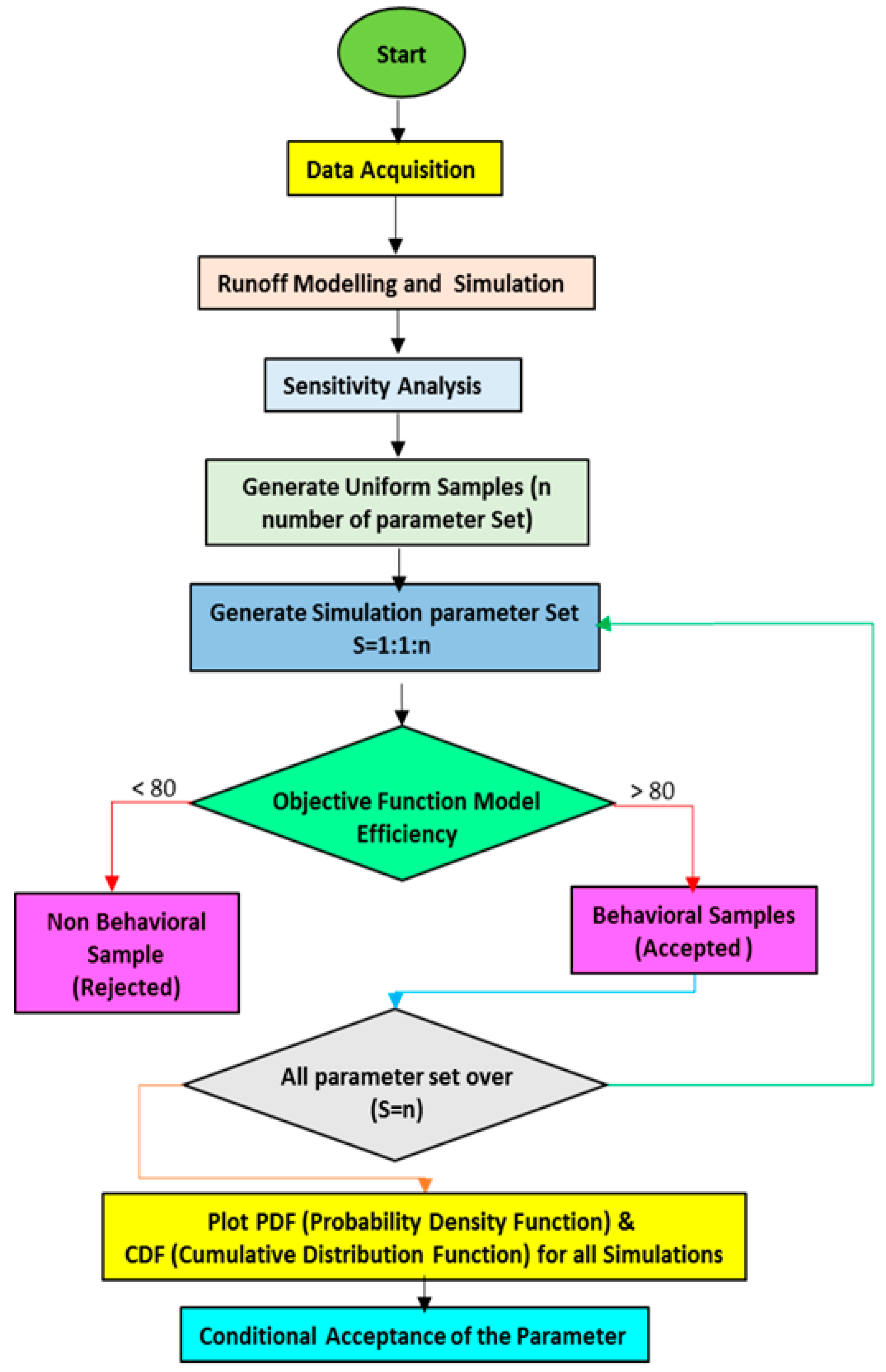
The uncertainty in HEC-HMS (Version 4.2.1) model parameters for the Astore catchment was determined using Monte Carlo analysis. When developing a forecasting model, certain assumptions are considered representing projections into the future, and the best option can be to estimate the expected value. It is not possible to know the actual value, but an estimate can be determined using historical data, expertise in the field, or past experience. This estimate is beneficial to developing a model, but entails some innate risk and uncertainty, since it is simply an estimate of an unknown value. Monte Carlo analysis is a method or technique used to recognize the effect of risk and uncertainty in various forecasting models. This analysis involves repeated generation of random parameters from probability distributions before computation of the output’s statistics. Only the more sensitive parameters (behavior samples) are considered, while other parameters are kept constant [35]. The possible combinations of all of the parameters are determined once the uniform random numbers of the parameters are generated. The values of each parameter set are entered into the rainfall-runoff model in order to determine the model’s efficiency. One or more efficiency criteria are used as objective function(s) during automated calibrations to help identify optimal parameter sets. Automated calibration refers to an approach in which the required model parameters are automatically generated, and the performance of the hydrological model or model efficiency is judged based on criteria defined by objective functions to assess the hydrological model simulation results. The objective functions that can be used for this purpose include NSE, RMSE, R², etc. Details about the model efficiencies and comparison were reported by Krause et al. [36]. In this case, the model efficiency is known as the objective function, which is to be minimized in the case of the root mean square error (RMSE) or maximized in case of the Nash–Sutcliffe efficiency (NSE). The process of the Monte Carlo analysis is presented in Figure 4.

To represent a real-world system, models use parameters that are numerical measures of characteristics or properties that do not change under definite conditions. The parameters of a model are considered to be its “turning knobs”, since they control the relationship between the inputs and output. The model’s parameter values can be adjusted during the calibration process to achieve accurate predictions. For example, a parameter in the HEC-HMS is the initial loss in the rate of the model. If this parameter is increased, the runoff decreases, and vice versa. The HEC-HMS parameters studied in this research include initial loss, imperviousness, time of concentration, and storage coefficient, all of which belong to the fitted model parameters.

The results from the HEC-HMS modeling serve as input (the general uniform sample, four parameters set) to estimate the parameter’s magnitude of uncertainty. The uncertainty analysis manager available in HEC-HMS 4.2.1 was used for this purpose, which is based on the Monte Carlo analysis.

Sensitivity analysis is a technique to assess how a model’s output variable(s) are affected by changes in the model parameters. This analysis aids in identifying the parameters that, if changed, will not affect the model output, and can therefore be fixed later or removed, which thus reduces the problems that can occur during the calibration phase of the modeling. The simulations differentiate the parameter sets into behavior samples (accepted) and non-behavior samples (rejected). The behavior sample regards the parameter set that produces a response (behavior) in the model that is similar to the response of the hydrological system. Similarly, non-behavior means that the parameter set will not cause a response similar to the hydrological system. The sensitivity analysis of a parameter is intended to compare the separation of the parameter values in behavior and non-behavior samples and the statistical Kolmogorov–Smirnov two-sample test can be used to estimate the significance of the separation [38]. Since the resulting distributions are not known, the two-sample test must be based on non-parametric methods.

The two-sample test is used to test whether two samples originate from the same distribution. The greater the separation, the more distinct the two samples. Suppose that the first sample has size m, with an observed cumulative distribution function of F(x), and that the second sample has size n, with an observed cumulative distribution function of G(x); then:

$$D_{m,n}=\underset{x}{\max }\left|F\left(x\right)-G\left(x\right)\right|$$

(1)

The null hypothesis H₀ supposes that the two distributions are equal, and if the resulting significance level of the test (α) is less than a certain specified value, the null hypothesis is rejected, that is, D_m,n > D_m,n,α, where D_m,n,α is the critical value [39,40]. The significance level, α, regards the probability of rejecting the null hypothesis when it is true. The significance level determines the difference in the results from the null hypothesis value. Under these conditions, the interpretation is that the model is sensitive to this parameter, since it is responsible for significant separation between behavior and non-behavior.

After simulation, all of the parameters were determined while probability density function and cumulative distribution function plots were generated from the results using Microsoft Excel 2013. Finally, a parameter set was conditionally accepted based on the statistical indicators or objective functions provided in

Table 2. Criteria for Evaluating the Performance of the Hydrological Model and their Corresponding Classifications.

Statistical Indicators	Value	Classification of Performance	Reference
Root Mean Square Errors (RSME) $RMSE=\sqrt{{\displaystyle {\displaystyle \sum }_{i=1}^n}\frac{{\left(Q_i^s-Q_i^o\right)}^2}{n}}$ $RSR=\frac{RMSE}{STDE{V}_{Obs}}$	value below half the standard deviation	Satisfactory	[47] [48]
	0.00≤ RSR ≤0.50	Very Good
	0.50 < RSR ≤ 0.60	Good
	0.60 < RSR ≤ 0.70	Satisfactory
	RSR > 0.70	Unsatisfactory
The correlation between actual and predicted values (R2) $R^2=1-\frac{\left(Q_i^o-Q_i^s\right)}{\left(Q_i^o-Q_{avg}\right)}$	0.85 to 1.00	Very Good	[49]
	0.70 to 0.85	Good
	0.60 to 0.70	Satisfactory
	0.4 to 0.60	Acceptable
	R2 ≤ 0.4	Unsatisfactory
Nash–Sutcliffe efficiency (NSE) $NSE=1-\frac{{{\displaystyle \sum }}_{i=1}^n{\left(Q_i^o-Q_i^s\right)}^2}{{{\displaystyle \sum }}_{i=1}^n{\left(Q_i^o-Q_{avg}\right)}^2}$	0.75 to 1.00	Very Good	[50] [48]
	0.65 to 0.75	Good
	0.50 to 0.65	Satisfactory
	0.4 to 0.50	Acceptable
	NSE ≤ 0.4	Unsatisfactory
Mean bias error (MBE) $MBE={\displaystyle {\displaystyle \sum }_{i=1}^n}\frac{\left(Q_i^s-Q_i^o\right)}{n}$	MBE > 0 (positive)	Overestimated Predictions	[51]
	MBE < 0 (negative)	Underestimated Predictions

.

2.5. Artificial Neural Networks (ANNs)

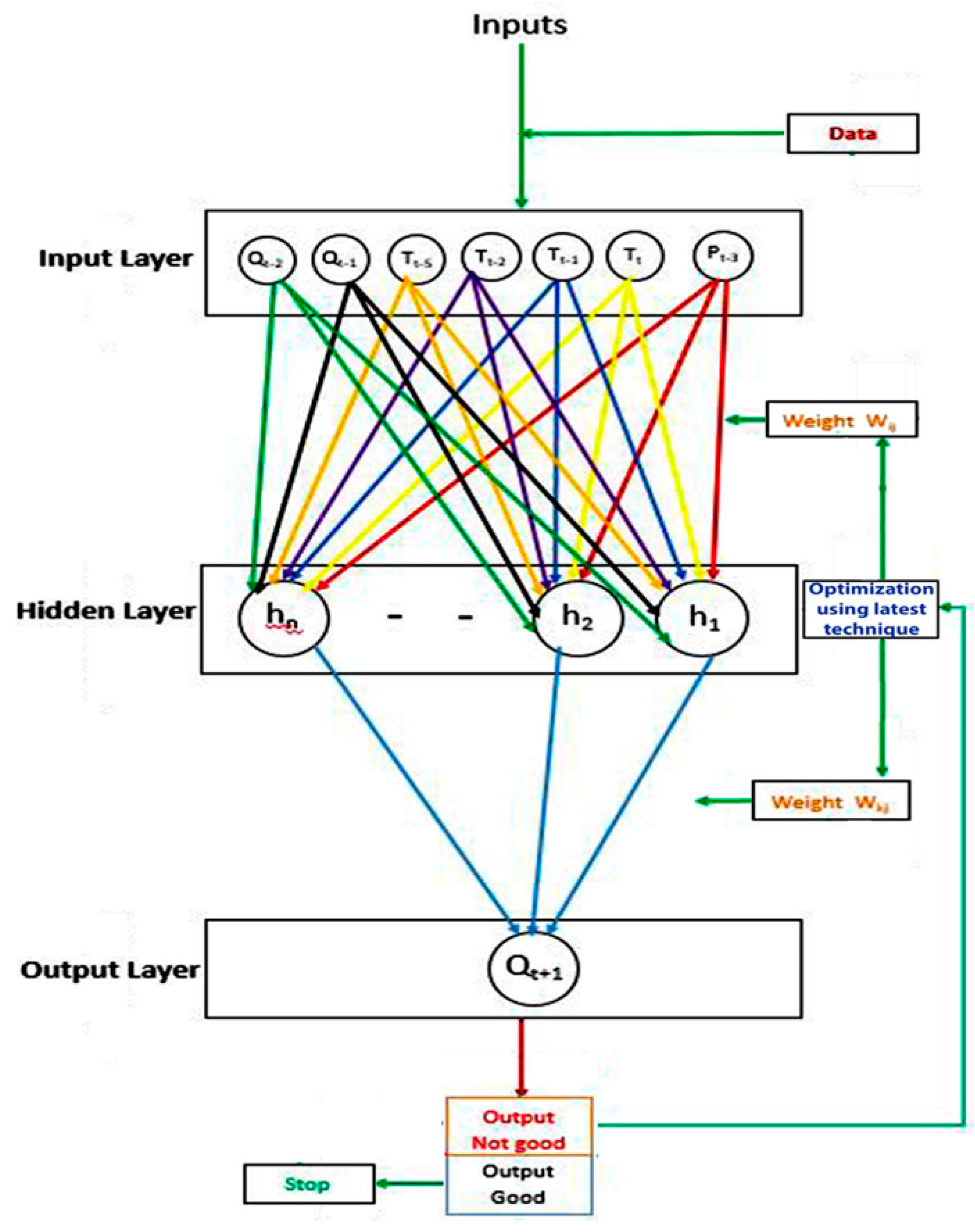
ANN models are used to address highly complex problems, and many investigators performing time-series hydrologic analyses have reported their success in establishing nonlinear relationships amongst input data and desired outputs [41,42,43]. ANN s consist of several “layers” of neurons, including an input layer with nodes representing various input variables, a hidden layer with many hidden nodes, and an output layer. The general architecture and a flowchart of ANNs are shown in Figure 5. For streamflow simulation, the ANN method requires selecting the best variables, functions, weights, and optimization techniques, which requires an objective function based on errors between the simulated and measured streamflow. Therefore, during the optimization process, the values of the parameters are selected so that the objective function achieves the minimum possible value (which is usually called the global minimum). A number of techniques are available to alter the parameters of the model in every iteration and search for the minimum value of the objective function. Derivatives of the objective function and constraints are used by some optimization techniques, while others do not require such derivatives and constraints. In streamflow prediction models, algorithms such as the quasi-newton, Levenberg–Marquardt, and conjugate gradient can be effectively utilized for standard numerical optimization due to its robustness [44,45]. In this study, the conjugate gradient training algorithm is used to simulate the streamflow for the Astore River Basin, and for comparison with the streamflow predicted from the HEC-HMS.

An efficient technique is required to select the best combination of input with respect to time lag. Monte Carlo analysis [46] has been used to select the input combination for the conjugate gradient-ANN model. The input data of the model is regarded as the observed daily rainfall for the Astore catchment. A tool enabling a Monte Carlo analysis interface with MS Excel was used to determine the required parameter samples. The parameters that were evaluated by the Monte Carlo analysis as behavior samples (having an objective function >80%) were accepted, while those falling under non-behavior samples (having an objective function <80%) were rejected. The measured streamflow data for the same river were used as the target during ANN model calibration and validation. Data from 1985 to 2004 were used for the calibration/ training and learning of ANN, while data from 2005 to 2014 were used for validation. The input combination obtained using Monte Carlo analysis provided better results than the input combination that was developed using coefficient correlation analysis in the previous research performed by the authors earlier this year [2].

2.6. Performance Evaluation of the Model

Many statistical indicators are used to evaluate model performance. Table 2 presents the indicators used in the current study. In the given relations, n stands for the total number of input samples, i represents the time series of the observed and simulated pairs, $Q_i^s$ and $Q_i^o$ stand for simulated and observed streamflow, and $Q$_avg is the observed average discharge in the stream.

3. Results and Discussion

3.1. Model Calibration

The Astore catchment was used to calibrate the model. Daily rainfall data for 20 years (1985–2014), constant monthly base flows of the river of the catchment for 20 years, and the catchment area were inserted into the model. The flows simulated from the methods were tested using statistical indicators (RMSE, MBE, R², NSE).

The statistical evaluation for calibration showed a satisfactory result in its RMSE values, but a very good result in R² and NSE, respectively. The MBE results indicate the overall prediction overestimation. The results are shown in

Table 3. Model Simulation Results for Calibration and Validation Periods.

Variable	Calibration Phase			Testing Phase
	Observed	Simulated	Residual	Observed	Simulated	Residual
Volume (×1000 m3)	91,447,988.3	87,490,381.7	3,957,606.6	47,324,538.1	39,594,381.3	7,730,156.8
Peak Flow (m3/s)	727.1	625.31	101.79	745.20	566.35	178.85
Date of Peak Flow	28 June 2003	28 June 2003		23 August 2010	23 August 2010

and

Table 4. Performance of the Model in Calibration and Validation Phases.

Statistics	Calibration		Validation
	Value	Performance	Value	Performance
R2	0.88	Very Good	0.79	Good
NSE	0.84	Very Good	0.70	Good
RSR	0.01	Very Good	0.01	Very Good
RMSE	0.58	Satisfactory	0.86	Acceptable
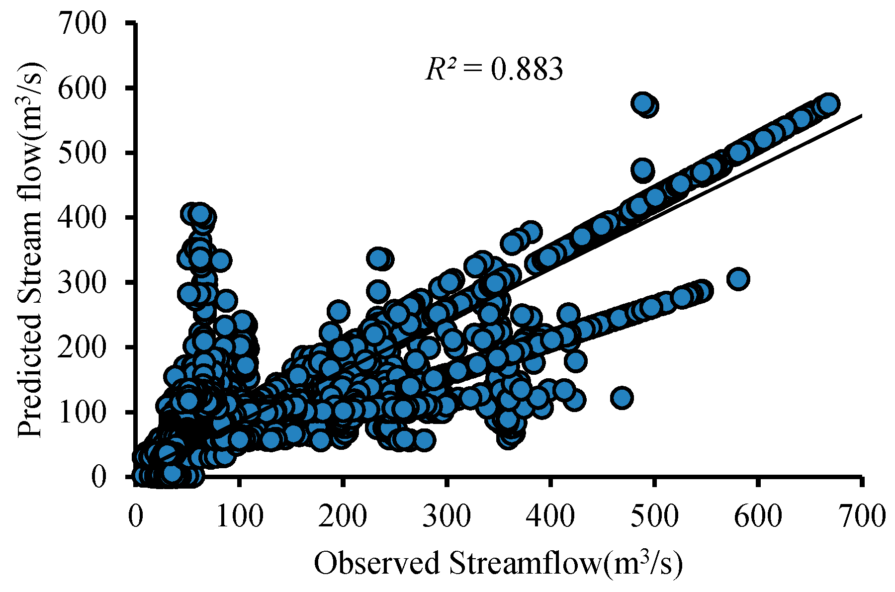
MBE	24.50	Over Estimation	39.30	Over Estimation

while the correlation analysis scatter plot is given in Figure 6. The observed and simulated hydrograph for the calibration period is shown in Figure 7, which assesses that the model estimated fewer flows during the summer and overestimated the flows in spring and autumn while more resembling flows during the winter. This is because the Astore catchment entails a considerable area comprised of glaciers that melt due to high temperatures in the summer, and contribute sufficient runoff to rainfall runoff during this period. The streamflow showed increasing trends versus temperature, while precipitation showed decreasing trends versus temperature; these results are supported by the literature review [52,53]. The positive trend in temperature is comparatively higher in winter than summer in the Upper Indus Basin [52]. It is reported that 16% to 53% of the total flow in the rivers generating from the western Greater Himalayas and the Hindu Kush are contributed by snow and glacier melt [54].

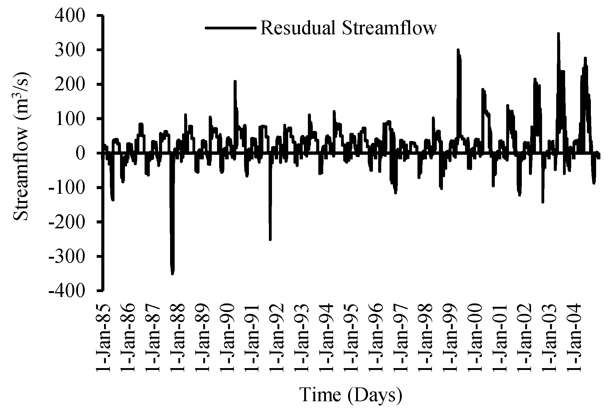
The flow residual graph further demonstrates this result (Figure 8). The positive residual flow clearly displays the underestimation of high flows (summer), while the negative residual flows represent overestimation flows during the spring and autumn seasons. The low estimated flows for both total flow volume and peak flow are shown in Table 3. The simulation of runoff is time-biased, which increases the errors in model performance assessments that are sensitive to outliers. The statistical evaluation for calibration found the model performance for the Astore watershed to be very good, since both R² and NSE >80% (Table 4).

3.2. Model Validation

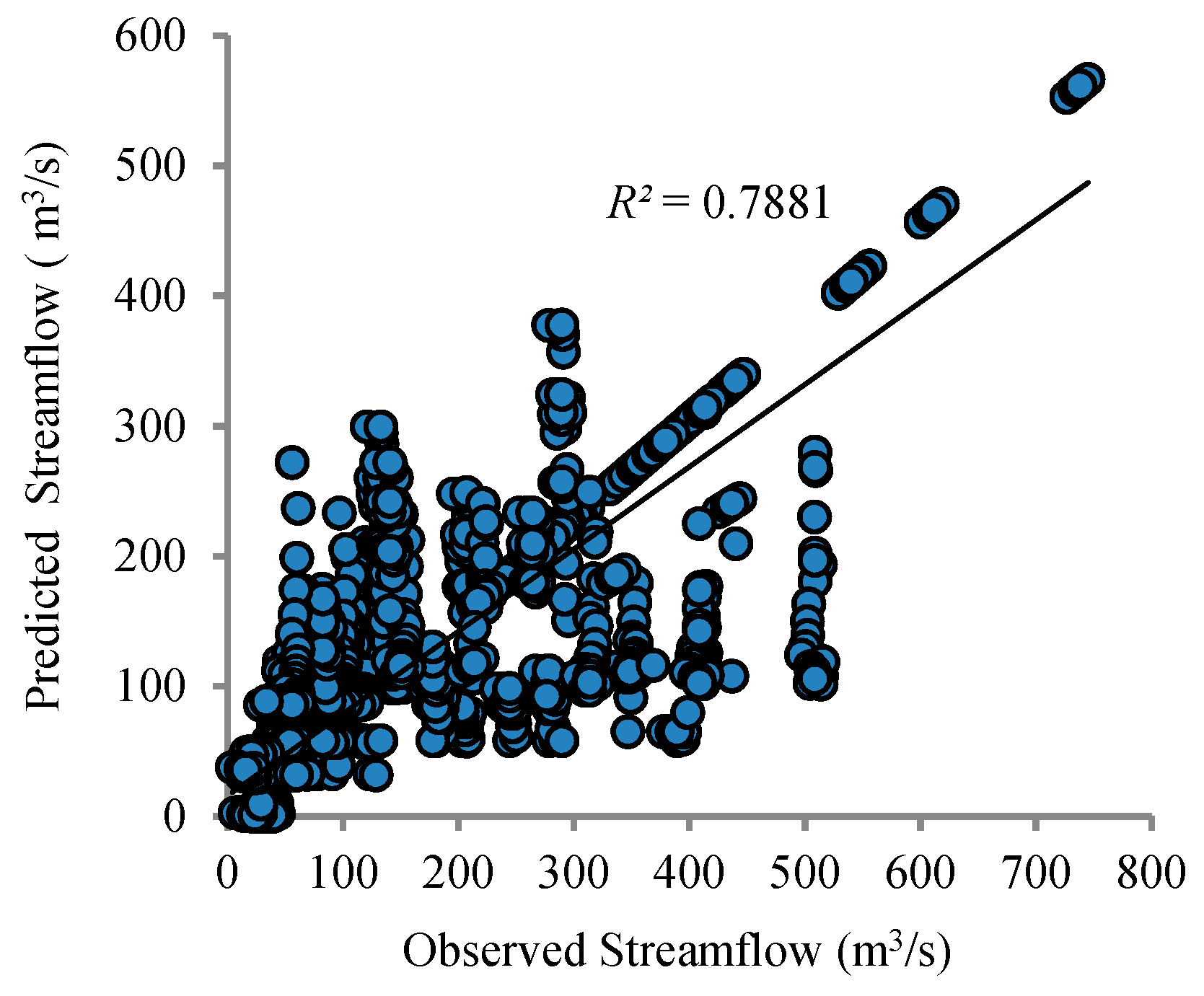
Employing the Clark unit hydrograph method for the years 2005–2014, the means of the observed flows, the simulated flows, and the values of statistical indicators for validation results are shown in Figure 9. The statistical indicators for the flow generated during the validation process show a bit lower performance than those in the calibration process. The estimated flows for both the total volume and the peak flow are given in Table 3. Since the R² >78% and NSE >69, the validated model performance for the Astore watershed is found to be good (Table 4).

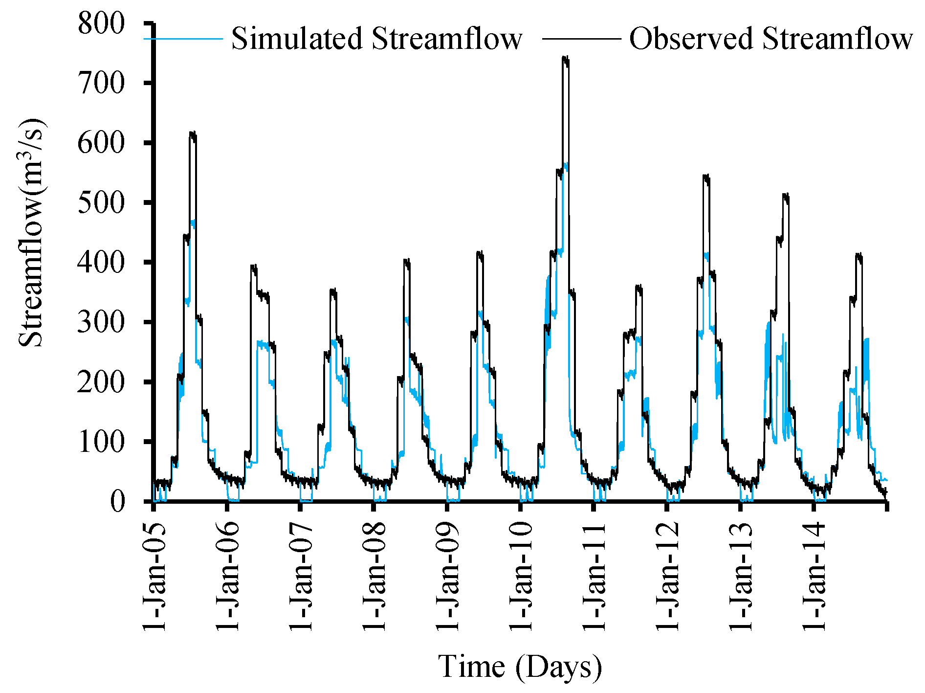
Observed and simulated flows for the validation period between 2005–2014 are also shown in Figure 10. The results for this validating period represent a similar pattern to that of the calibration period, with satisfactory values of statistical indicators. However, it shows underestimated flows in summer, but comparatively fewer overestimated flows in spring and autumn (Figure 10).

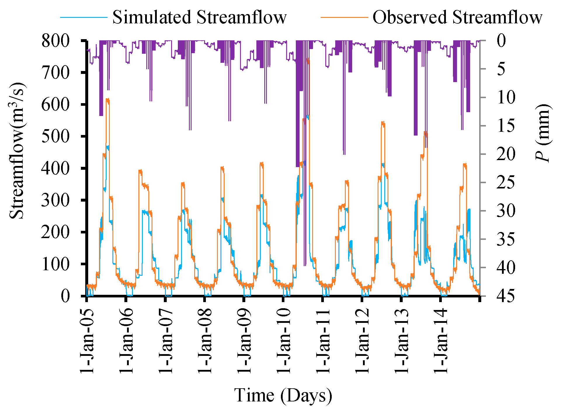
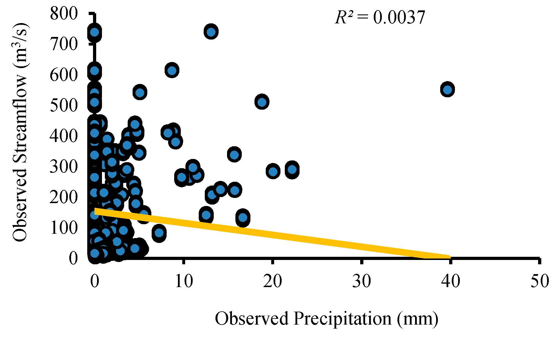
Figure 11, Figure 12, Figure 13 and Figure 14 describe the relationship between precipitation and temperature with observed and simulated streamflow. The figures clearly show that both precipitation and temperature impact runoff. When rainfall is zero, streamflow is never zero, and there is considerable runoff in the study region, which is obviously due to the melting of the glacier part of the catchment as a result of the comparatively high temperatures during the summer season and obtaining a mostly subsurface flow at the Doyian gauging station.

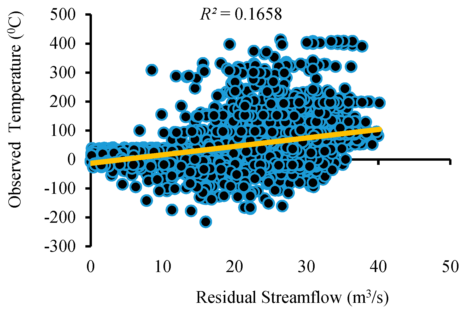
Figure 11, Figure 12, Figure 13 and Figure 14 also show a decreasing trend in the rainfall runoff as a result of increasing temperatures in the region. The result shows a proportional relationship between streamflow and temperature during the validation period (Figure 12). It is evident from Figure 15 that residual streamflow/runoff (the flow in excess of the rainfall) is due to the melting of glaciers caused by increasing temperatures in the region throughout the year.

3.3. Sensitivity Analysis

Table 5. Output of the HEC-HMS Parameters.

Parameters	Minimum	Maximum	Mean	Standard Deviation
Initial abstraction (mm)	0.02	64.46	33.14	18.47
Imperviousness (%)	63.89	99	81.22	10.15
Time of concentration (h)	5.75	8.24	7.00	0.71
Storage coefficient (h)	10.83	31.24	25.05	3.63

summarizes the HEC-HMS calibrated parameters, showing significant yield agreement between the observed and estimated flows. The results of Monte Carlo analysis for these parameters are shown in

Table 6. Results of Monte Carlo Analysis with 500 Trials.

Parameters	Initial Loss (mm)	Imperviousness (%)	Time of Concentration (h)	Storage Coefficient (h)
Mean	33.14	81.22	7.00	25.05
Number of Trials	500.00	500.00	500.00	500.00
Standard Error	−0.67	−0.22	0.00	0.08
Minimum	0.02	63.89	5.75	10.83
Maximum	62.46	98.98	8.24	31.24
Median	34.60	81.07	7.01	25.03
Range	62.44	35.09	2.49	20.41
Standard Deviation	18.47	10.15	0.71	3.63
Variance	341.29	103.11	0.50	13.20
Skewness	−0.12	0.03	−0.05	−0.11
Kurtosis	−1.22	−1.19	−1.20	−0.82

and Figure 16. From the sensitivity analysis, the initial loss was found to be from 0.02 mm to 64.46 mm (mean: 33.14 mm). In case of imperviousness, the initial loss ranged from 63.89% to 98.98% (mean: 81.22%). The simulation values for the time of concentration were found to be in the range of 5.75 h to 8.24 h (mean: 7 h). The storage coefficient includes values from 10.83 h to 31.24 h, with a mean value of 25.05 h. The sensitivity quantified from this study regarding different parameters and their results in form of statistical indicators can be utilized to improve the future modeling processes.

3.4. ANN Modeling

To predict the daily streamflow, the measured precipitation (P) and Temperature (T) with various time (t in days) lags (T_t, T_t−1, T_t−2, T_t−3, T_t−4, T_t−5, P_t, P_t−1, P_t−2, P_t−3, P_t−4, P_t−5) were used as input variables, and streamflow (Q_t+1) was used as the output variable.

In the present paper, Monte Carlo analysis is used to determine the input combination for the conjugate gradient ANN model. The parameters evaluated by Monte Carlo analysis as behavior samples were accepted while non-behavior samples were rejected; hence, the input variables P_t−3, T_t, T_t−1 and T_t−5, show similar behavior to the hydrological system with respect to the output parameter (Q_t+1).

The performance of the ANN model was analyzed using various indicators (e.g. R², RMSE, NSE, and MBE) and selected input combinations. The determined index values are shown in

Table 7. Indices for the Input Combination Predicted for Conjugate Gradient-ANN Modeling Based on Monte Carlo Analysis.

Statistics	Training	Testing
	Value	Value
R2	0.85	0.75
NSE	0.79	0.70
RMSE	0.78	0.79
MBE	19.19	9.15

, with the best values in bold. The range of values of the four statistical indicators infer that it is impossible to use a unique statistical indicator to define model performance, as the model shows no excellent values amongst the four. However, the indices show that the selected input combination produced acceptable accuracy, which demonstrates the high efficiency of selecting algorithms of Monte Carlo analysis and the ANN models. The accuracy depends on the chosen input and optimization method used in the ANN. As the optimization method’s efficiency increases, it provides improved accuracy to the simulated streamflow. It is noteworthy that combining Monte Carlo analysis and the efficient optimization technique conjugate gradient significantly improves the performance of the ANN model.

3.5. Comparison of ANN and HEC-HMS

The performance of the ANN model was compared with the HEC-HMS results using four statistical parameters (R², RMSE, MBE, and NSE). The values of the statistical indicators for ANN and HEC-HMS are given in

Table 8. Comparison of Index Values of ANN and HEC-HMS Modeling for Validation Period.

Statistics	HEC-HMS	ANN
R2	0.79	0.75
NSE	0.70	0.70
RMSE	0.86	0.79
MBE	39.30	9.15

The best results are highlighted in bold.

and Figure 17, and Figure 18a,b. A comparison of the observed and predicted streamflow for the calibration/training and validation/testing phases of various ANN and HEC models is presented in Figure 19. The high value of statistical indicators (i.e., R², RMSE, MBE, and NSE) indicates that the efficiency of the HEC-HMS model is better than that of the conjugate gradient ANN.

3.6. Flow Duration Curve Analysis

Streamflow from the River Indus is highly useful for irrigated agriculture and hydropower generation [54,55]. 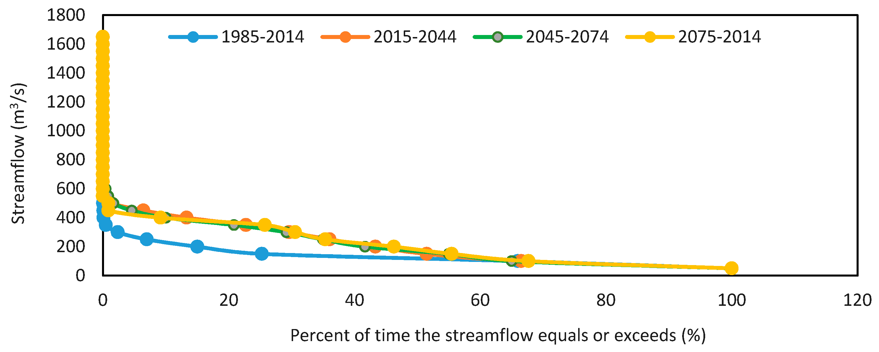A flow duration curve is an important component for designing hydropower and represents the relation between the magnitude and frequency of daily streamflow for a particular river basin, which evaluates the percentage of time that it takes for a certain streamflow becomes equaled or exceeded over a historical period [56]. The flow duration curve produces a detailed graphical view of the complete historical changes related to streamflow in a river basin. The profile of the flow duration curve for any river thoroughly reveals the type of flow system and influences the characteristics of the upstream catchment including the geology, urbanization, artificial influences, and groundwater. Therefore, in order to construct the flow duration curve, the streamflow was plotted against the percentage of the exceedance scale, as illustrated in Figure 20 and Figure 21. Comparisons of the flow duration curve plotted from discharges predicted by HEC-HMS and ANN modeling with the flow duration curve plotted from the observed flow rate and the profiles of the three flow duration curves clearly reveal the complete historical changes related to streamflow in the Astore river basin. Considering the flow duration curve plot, the flow at 0–25% exceedance was over 250 m³/s and 150 m³/s in the HEC-HMS and ANN predictions, respectively, which is a higher flow rate and may result in extreme events. For a few months of the year, this flow rate or higher at almost 95% exceedance is about 45 m³/s, which is the lowest flow rate record, and may cause droughts for some time. So, by definition, the river flows at this rate for 95% of the time or more. Familiarity with the flow duration curve will help provide knowledge needed for hydrologic studies such as hydropower, water supply, irrigation planning, river and reservoir sedimentation, sustainability of habitats, and water deliveries through the reservoirs. Figure 20 obviously shows that the flow duration curve has changed significantly when modeled by the HEC-HMS as compared to the ANN.

3.7. Discussion on Results (Comparison with Other Research Work)

More than one statistical indicator was used to judge the performance of the models, as it was necessary to test the models based on various aspects. For example, statistical evaluation during calibration indicated a satisfactory result on the basis of the RMSE, value but a very good result in cases of R² and NSE, respectively. Adnan et al. [57] observed a similar pattern that supports the idea of avoiding using a single statistical indicator for performance evaluation of rainfall runoff models. Regarding calibration, a sensitivity analysis of hydrologic model parameters was performed. The results show that the time of concentration and storage coefficient regard the most influencing parameters of a hydrologic model must be estimated with a very high accuracy. Rathod and Manekar [37] identified that the imperviousness of the catchment area is the least influencing parameter. According to Wang and Solomatine [58], the time to peak is the most influential model parameter, while Ghumman et al. [1] observed that the kinematic wave parameter is the most contributing hydrologic element in rainfall runoff modeling. This discussion shows that it is wise to perform a sensitivity analysis of hydrologic model parameters for each catchment in order to achieve better understanding of rainfall-runoff behavior.

Following calibration, the models were compared with each other. Both the data-driven ANN models and distributed hydrologic models entail their merits and demerits. The HEC-HMS model is comparatively more efficient than ANN; however, the HEC-HMS requires a significant effort to determine the model parameters. Jimeno-Sáez et al. and Derdour et al. [2,59] report similar findings when comparing a soil and water assessment tool (hydrologic model) with the ANN.

4. Summary and Conclusions

This paper discusses runoff simulation in the Astore watershed of Pakistan’s Upper Indus River Basin using data from 1985 to 2014. The runoff simulation was investigated with the help of Quantum Geographic Information Software to delineate the digital elevation model that was imported to the HEC-HMS. Daily precipitation and temperature time-series data were used as input for a period of 20 years (1985–2004) for calibrating, and the next 10 years (2005–2014) for validating the model. The streamflow model was evaluated by mean bias error (MBE), Nash–Sutcliffe Efficiency (NSE), root mean square error (RMSE), and the (R²). The results demonstrated that the model estimated much lower flows during the summer, and higher flows during winter. This is because the Astore catchment entails a considerable glacial area that melts due to high temperatures in the summer and results in contributing sufficient runoff to the rainfall runoff during the respective period. Decreasing trends of the rainfall-runoff pattern as a result of increasing temperatures were observed in the region, and the results showed the proportional relation between streamflow and temperature during the validation period.

For the sensitivity analysis, four parameters were investigated: initial loss, imperviousness, time of concentration, and storage coefficient. The mean, standard deviation, and range of these parameters were determined. Sensitivity analysis using Monte Carlo analysis was performed on these parameters, and their sensitivity was determined using 500 trials assuming simple distribution. The most important parameters were found to be the storage coefficient and time of concentration, which are interrelated.

Furthermore, the ANN and HEC-HMS were applied to develop models for predicting streamflow. Monte Carlo analysis was used to predict the best input combination for streamflow forecasting. The performance of the ANN models was compared with the HEC-HMS results using four statistical indicators (R², RMSE, MBE, and NSE). The HEC-HMS model was found to be comparatively more efficient than the conjugate gradient ANN.

The flow duration curves were plotted for the predicted streamflow, which presents the complete historical changes related to streamflow in the river basin. It was evaluated that extreme events (floods and droughts) are expected to occur in the studied river basin in the near and distant future. Familiarity with the details of the flow duration curve will aid in understanding the characteristics of a river basin and the knowledge needed in hydrologic studies.

In order to better estimate summer and autumn flows, further research is recommended to simulate the seasonal runoff in the Astore basin while considering the solid snowpack runoff volume (glacier melt). In addition, the results of this work can be used in future streamflow modeling exercises to narrow the range of parameters to be investigated by the modeler. Moreover, the results obtained from the ANN model as well as Monte Carlo analysis should be compared against other input selection methods (e.g., principal component analysis and fuzzy system).