Extraction of Urban Water Bodies from High-Resolution Remote-Sensing Imagery Using Deep Learning


Abstract
1. Introduction
- (1)
- A novel extraction method for urban water bodies based on deep learning is proposed for remote-sensing images. The proposed method combines the superpixel method with deep learning to extract urban water bodies and distinguish shadow from water.
- (2)
- A new CNN architecture is designed, which can learn the characteristics of water bodies from the input data.
- (3)
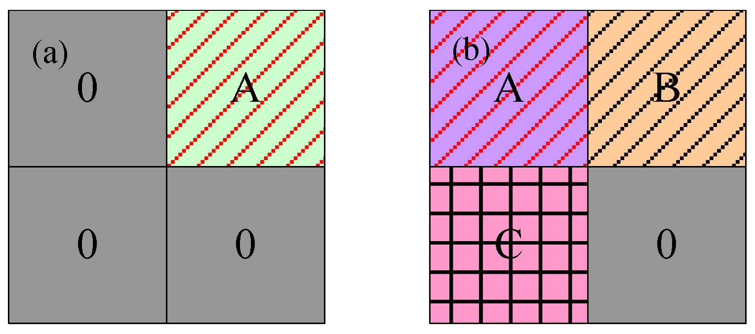
- In order to reduce the loss of image features during the process of pooling, we propose self-adaptive pooling (SAP).
2. Materials and Methods
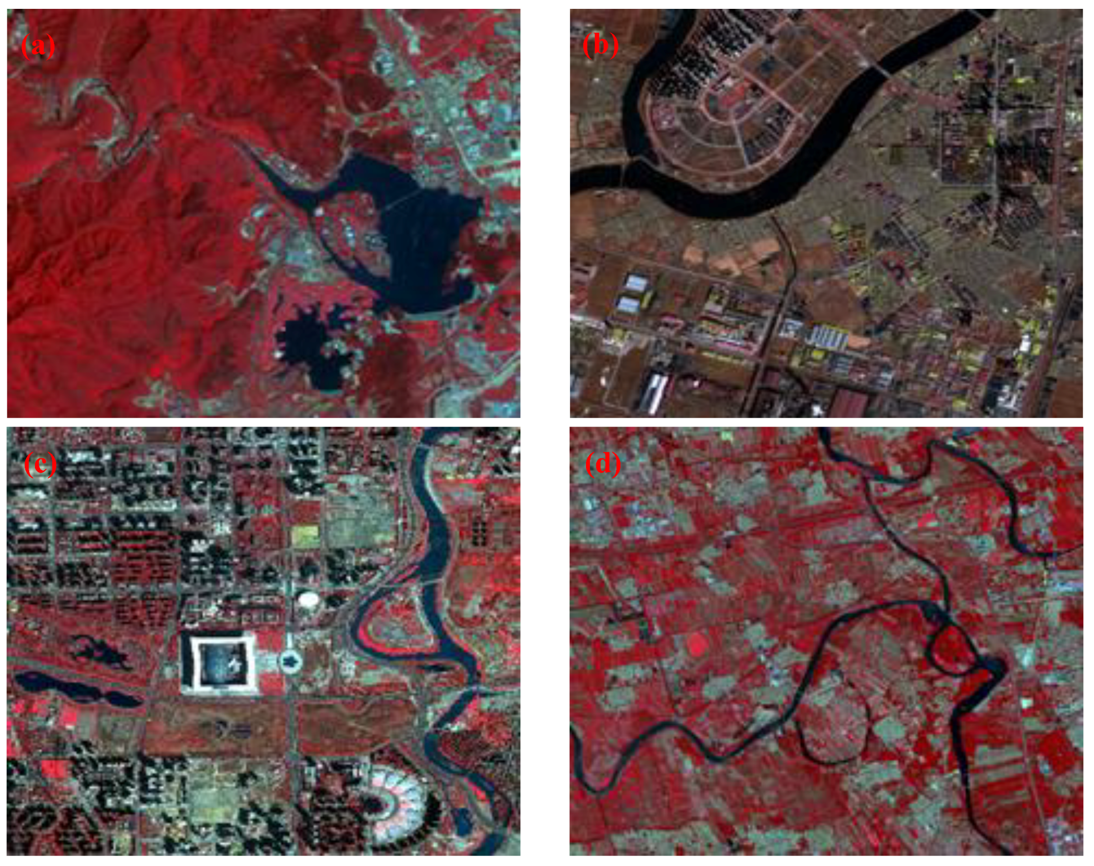
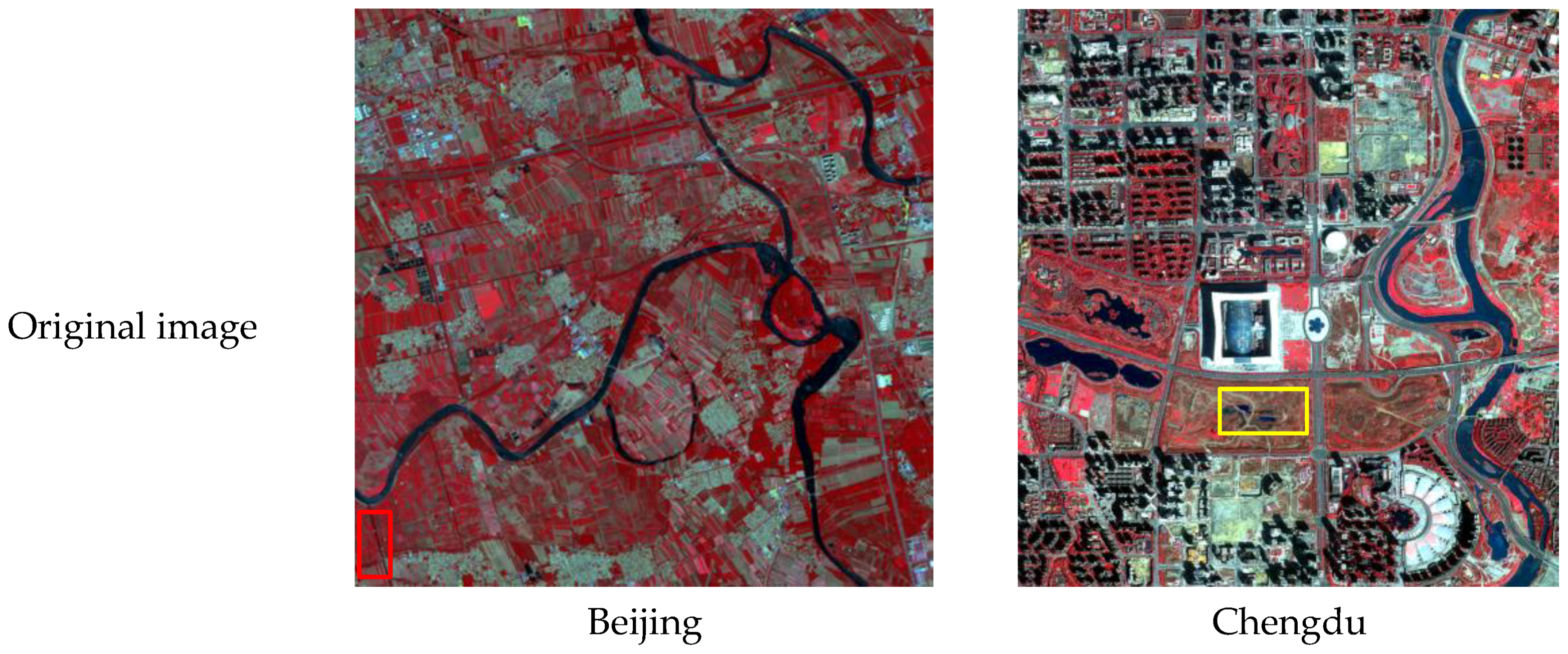
2.1. Study Areas
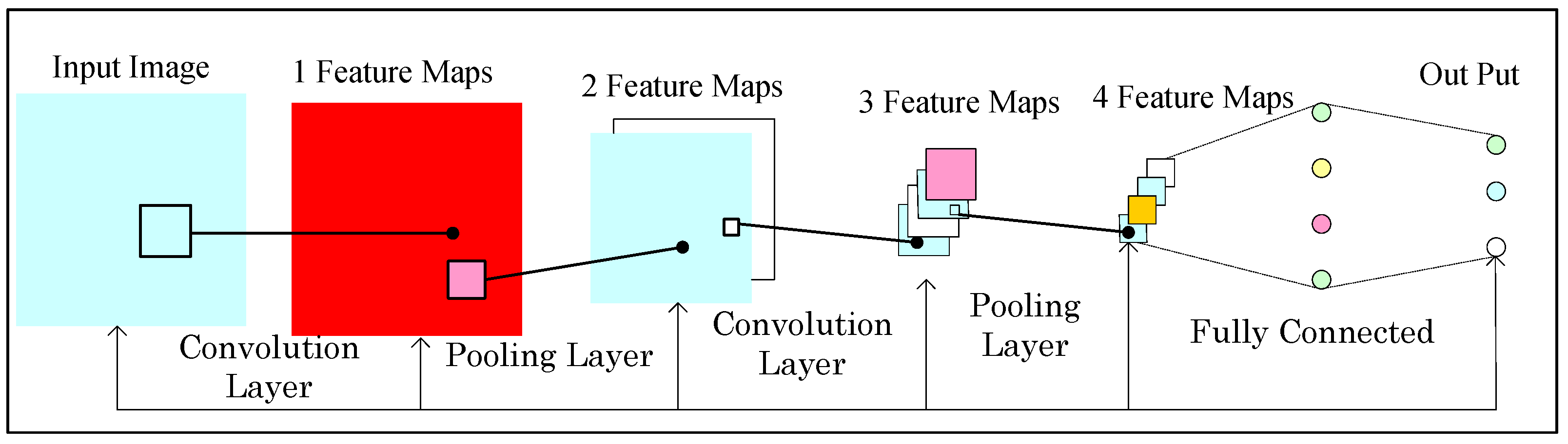
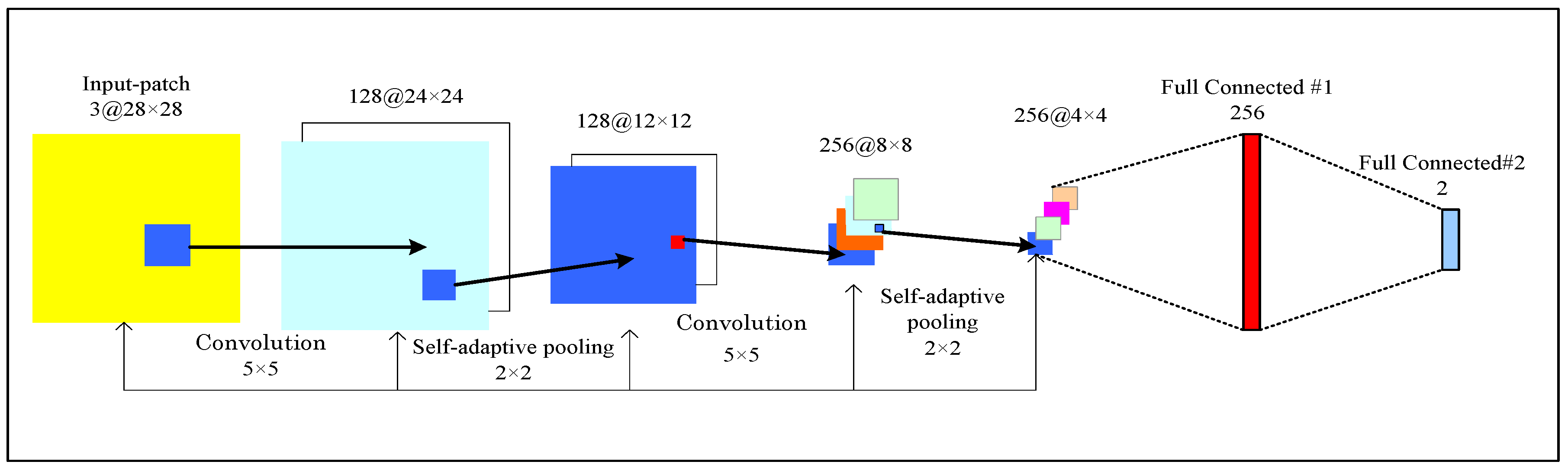
2.2. Self-Adaptive Pooling Convolutional Neural Networks (CNN) Architecture
2.3. Pre-Processing
2.3.1. Color Space Transformation
2.3.2. Adaptive Simple Linear Iterative Clustering (A-SLIC) Algorithm
- Step 1. For an image containing pixels, the size of the pre-divided region in this algorithm is , then the number of regions is . Each pre-divided area is labeled as . In this paper, and are defined zero, and is defined one.
- Step 2. HIS transformation is performed on each pre-divided area. In the th region, according to Equation (10), the similarity between two pixels is calculated in turn.
- Step 3. According to Equations (14) and (16), the sum of and is calculated and the iteration begins.
- Step 4. If and no longer change or reach the maximum number of iterations, the iteration is terminated. The point where the sum of and is max is regarded as the cluster center (, where ).
- Step 5. Repeat steps 3 to 4 until the entire image is traversed, and adaptively determine the number of superpixels (). In this paper, the HSI value are the center of the pixel. Finally, complete the superpixel segmentation.
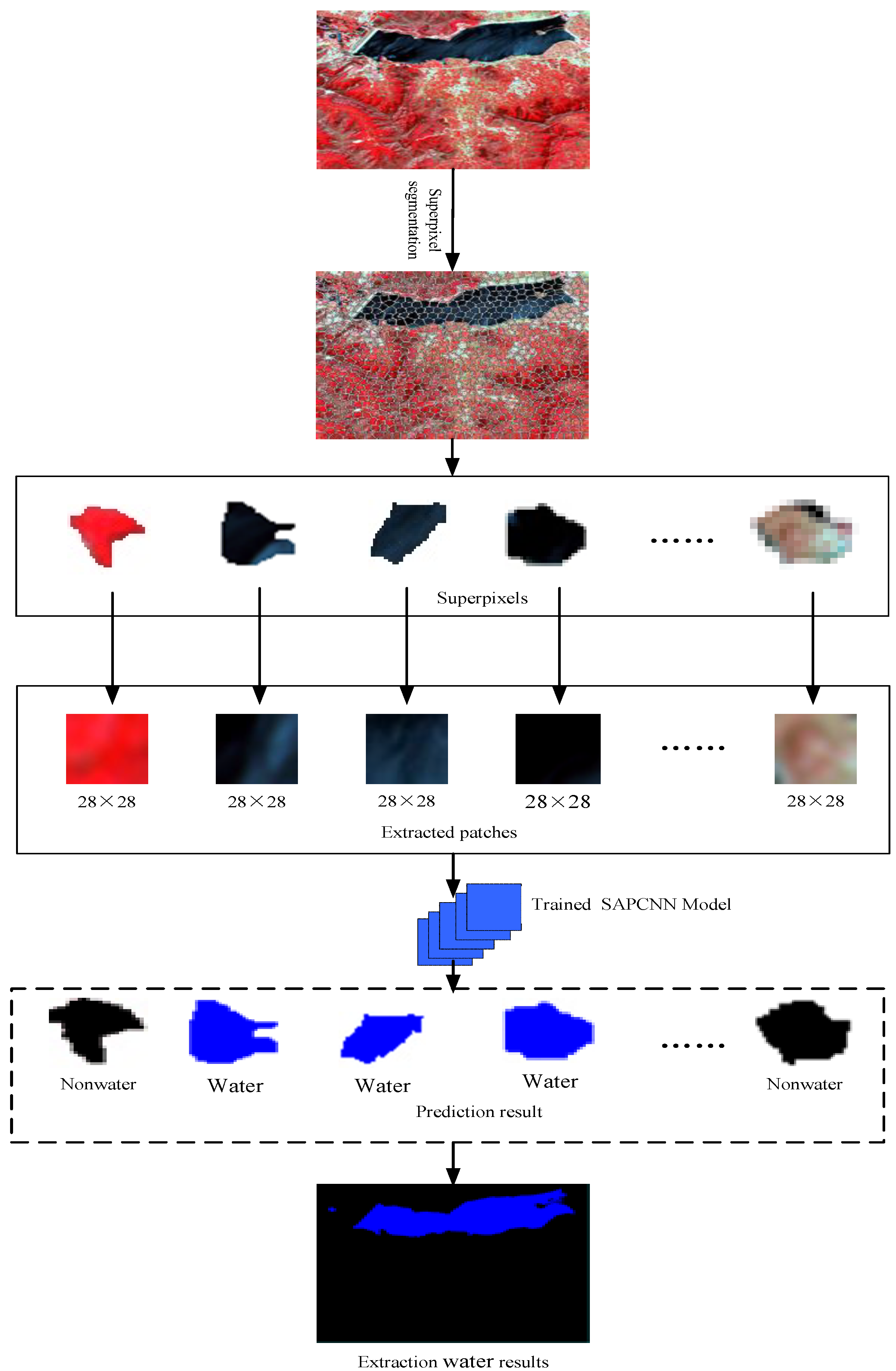
2.4. Network Semi-Supervised Training and Extraction Waters
2.5. Accuracy Assessment Method
- : true positives, i.e., the number of correct extraction pixels;
- : false negatives, i.e., the number of the water pixels not extracted;
- : false positives, i.e., the number of incorrect extraction pixels;
- : true negatives, i.e., the number of no-water bodies pixels that were correctly rejected.
3. Experiments and Discussion
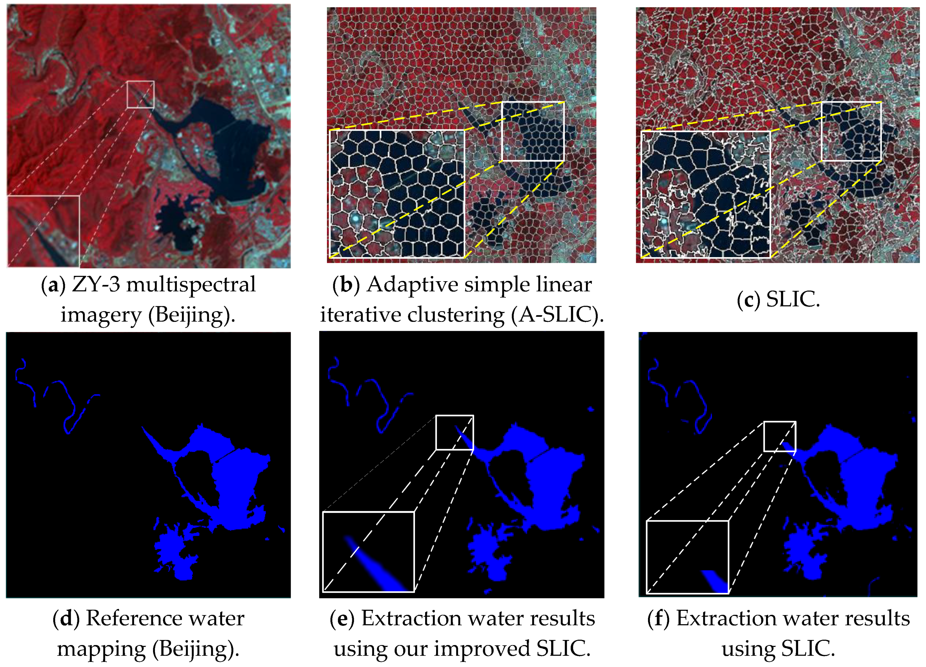
3.1. Impact of the Superpixel Segmentation on the Performance of Water Mapping
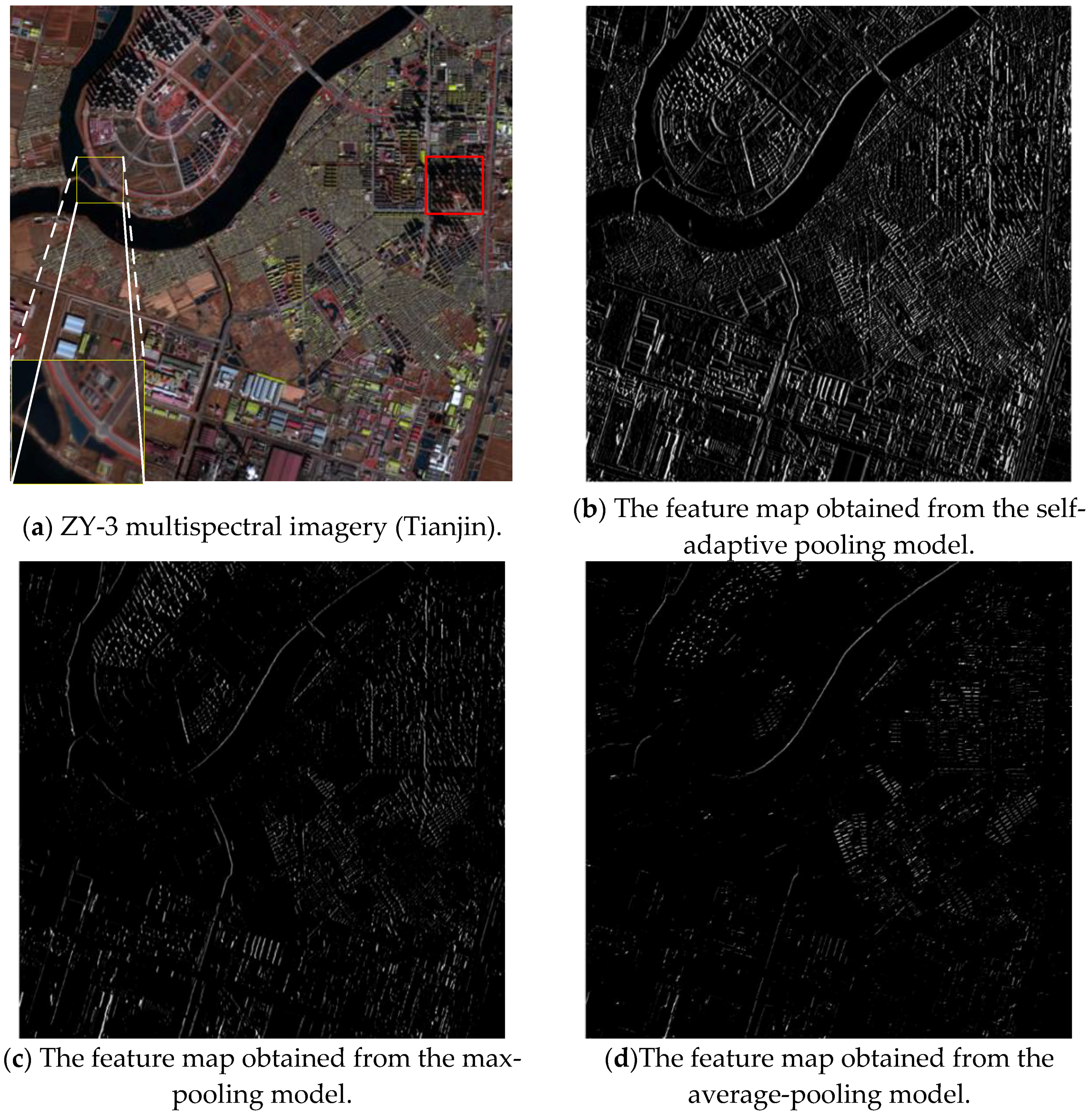
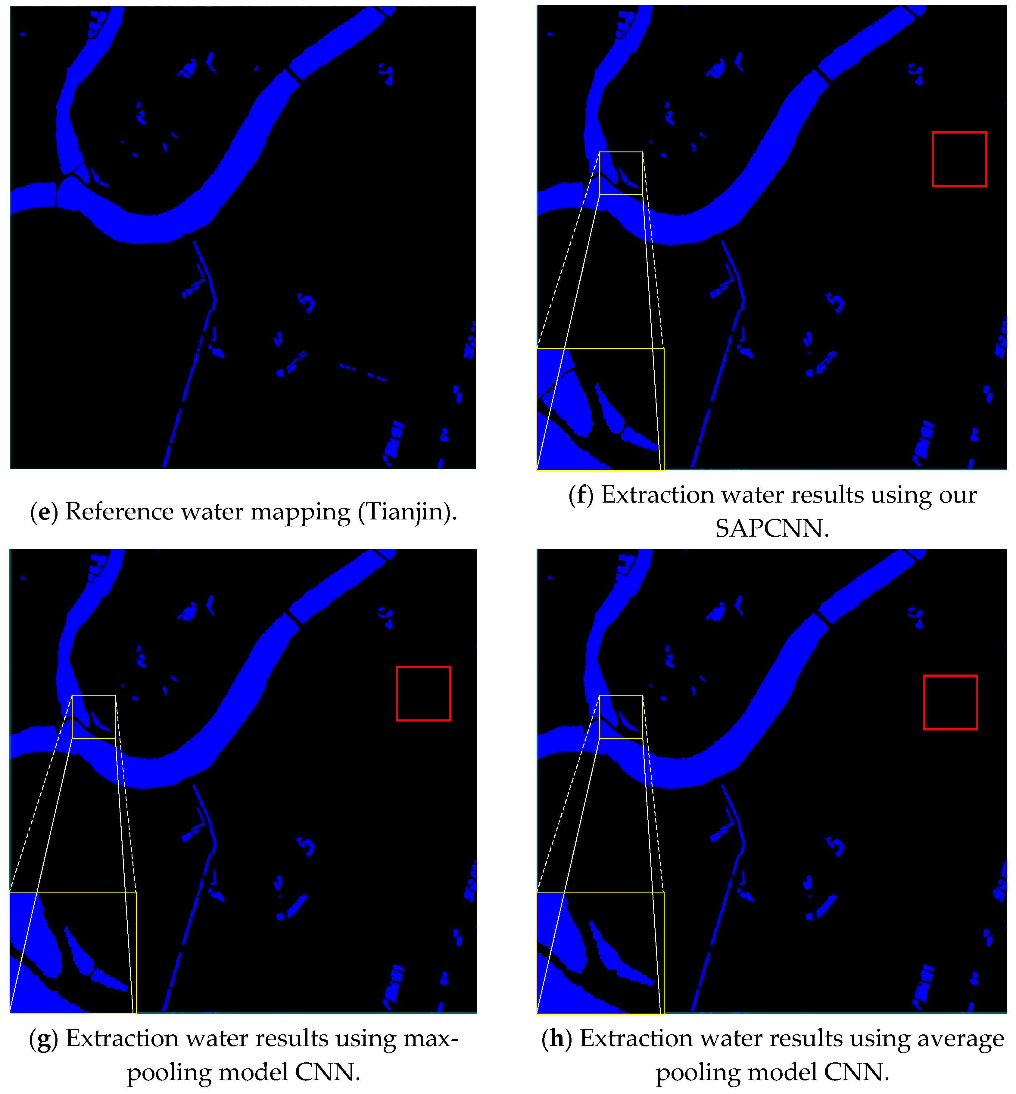
3.2. Comparison between Different Model CNN Architectures
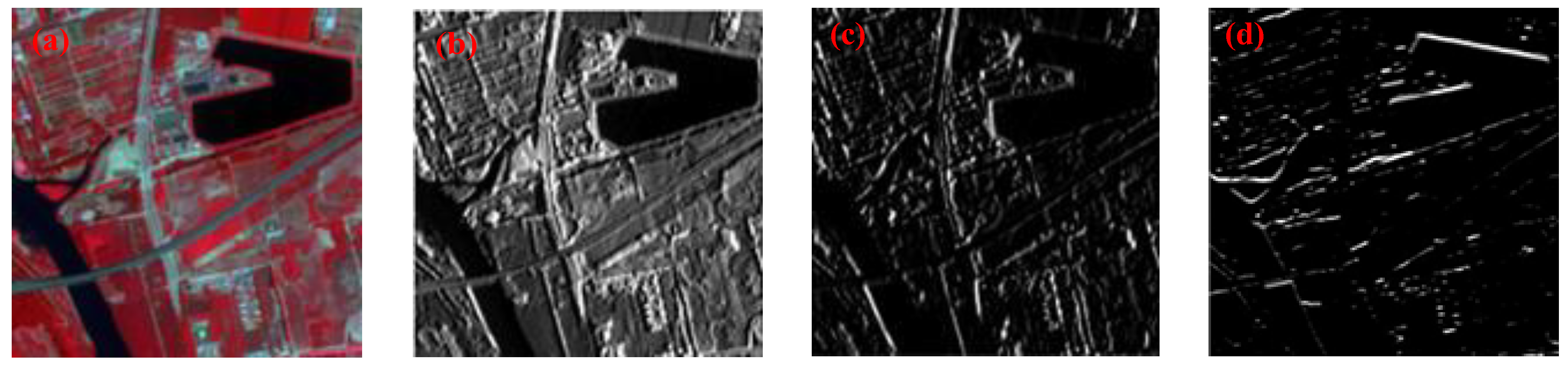
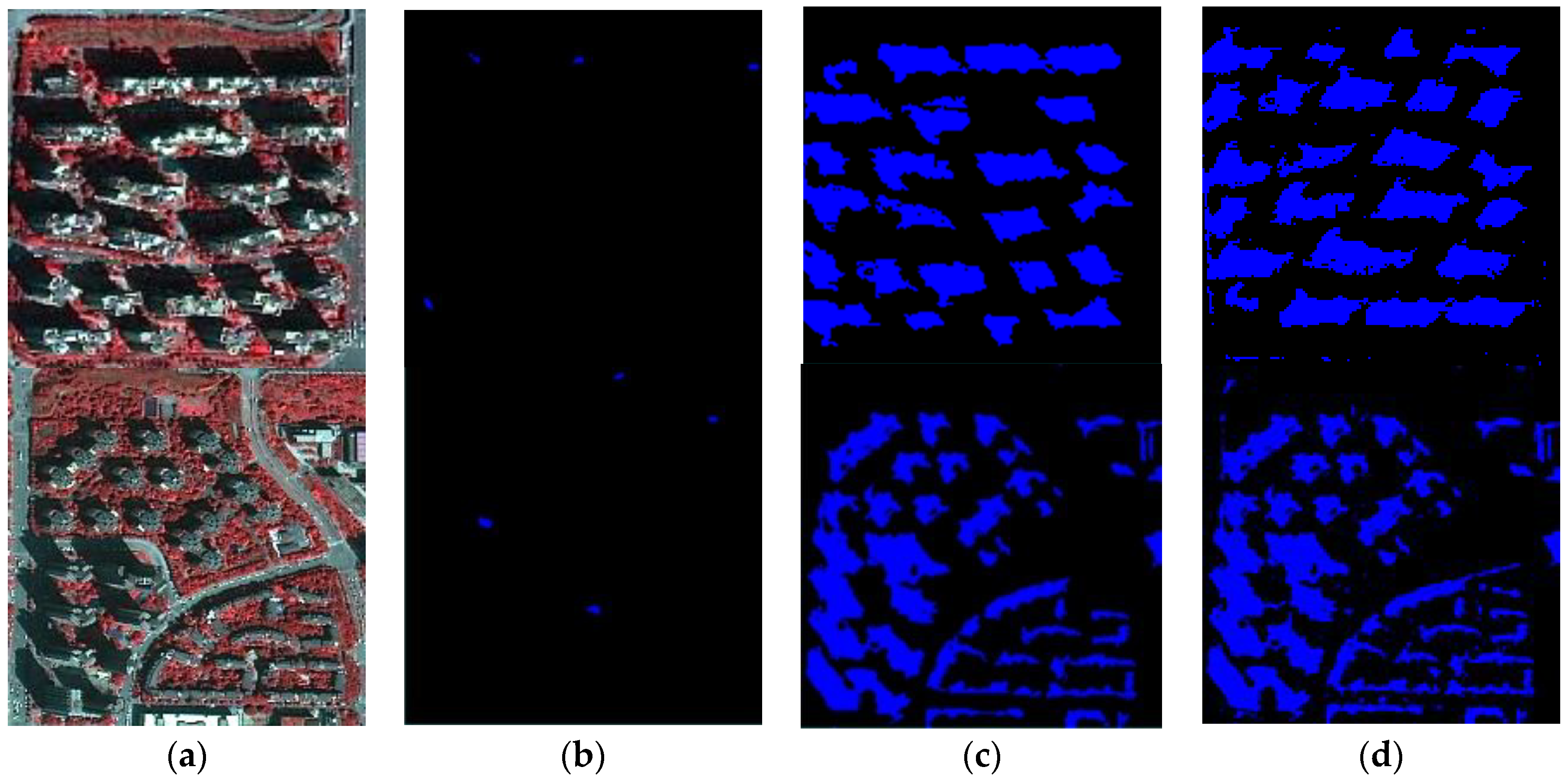
3.3. Distinguishing Shadow Ability of Different Methods
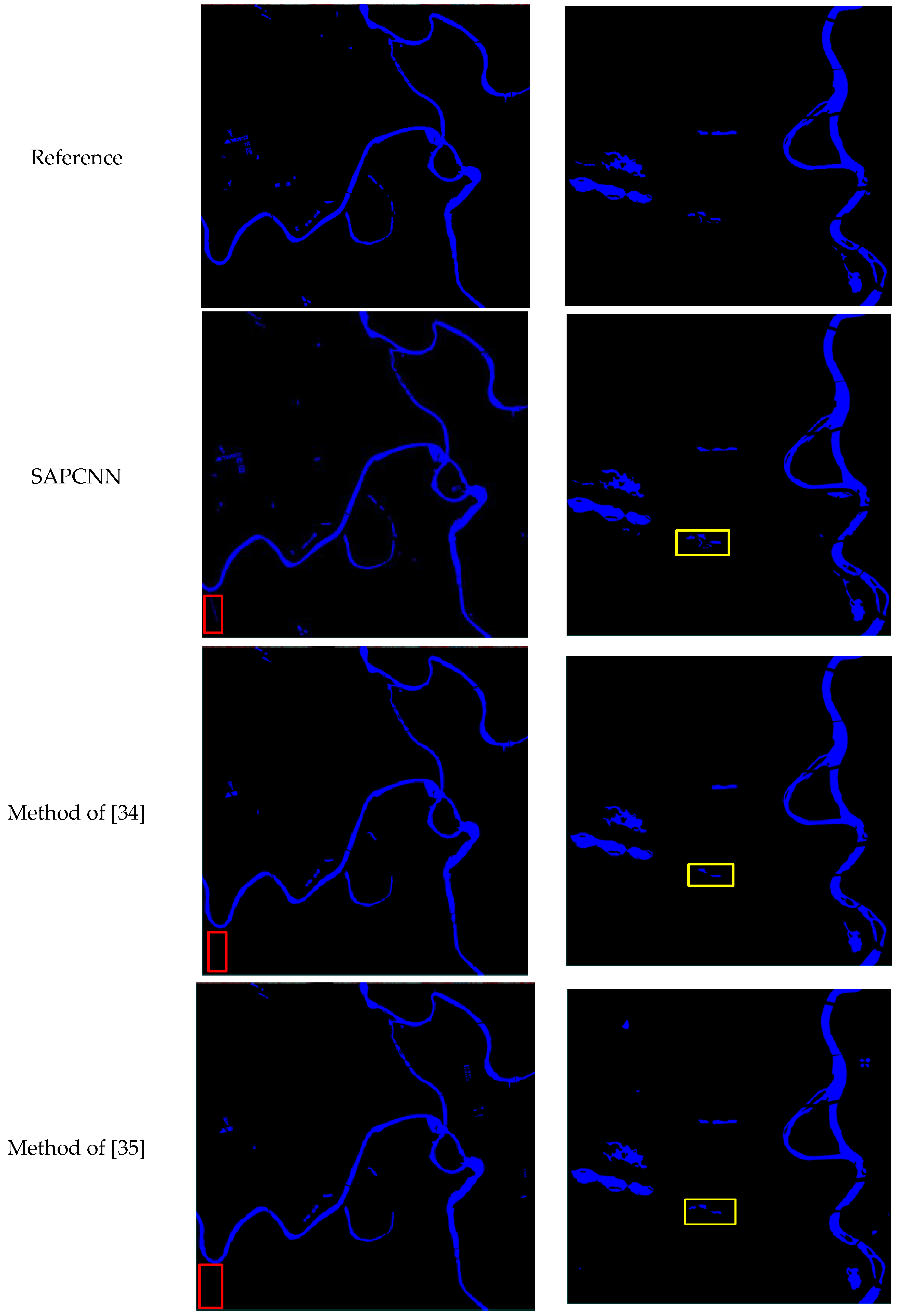
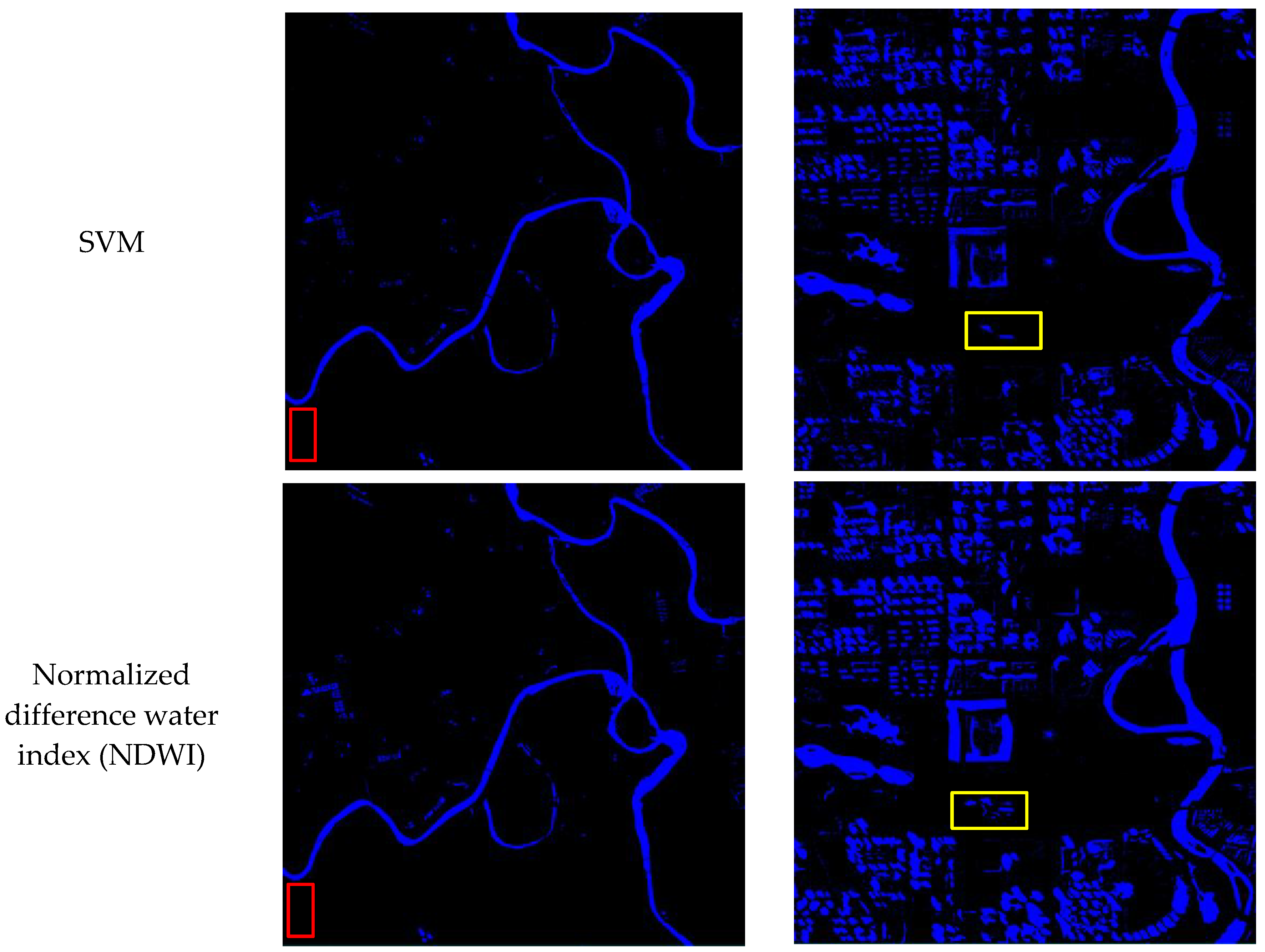
3.4. Comparison with Other Water Bodies Extraction Methods
4. Conclusions
Author Contributions
Acknowledgments
Conflicts of Interest
References
- Fletcher, T.D.; Andrieu, H.; Hamel, P. Understanding, management and modelling of urban hydrology and its consequences for receiving waters: A state of the art. Adv. Water Res. 2013, 51, 261–279. [Google Scholar] [CrossRef]
- Rizzo, P. Water and Wastewater Pipe Nondestructive Evaluation and Health Monitoring: A Review. Adv. Civ. Eng. 2010, 2010, 818597. [Google Scholar] [CrossRef]
- Byun, Y.; Han, Y.; Chae, T. Image fusion-based change detection for flood extent extraction using bi-temporal very high-resolution satellite images. Remote Sens. 2015, 7, 10347–10363. [Google Scholar] [CrossRef]
- Yang, X.; Zhao, S.; Qin, X.; Zhao, N.; Liang, L. Mapping of Urban Surface Water Bodies from Sentinel-2 MSI Imagery at 10 m Resolution via NDWI-Based Image Sharpening. Remote Sens. 2017, 9, 596. [Google Scholar] [CrossRef]
- Du, Y.; Zhang, Y.; Ling, F.; Wang, Q.; Li, W.; Li, X. Water bodies’ mapping from Sentinel-2 imagery with Modified Normalized Difference Water Index at 10-m spatial resolution produced by sharpening the SWIR band. Remote Sens. 2016, 8, 354. [Google Scholar] [CrossRef]
- Zhou, Y.; Luo, J.; Shen, Z.; Hu, X.; Yang, H. Multiscale water body extraction in urban environments from satellite images. IEEE J. Sel. Top. Appl. Earth Obs. Remote Sens. 2014, 7, 4301–4312. [Google Scholar] [CrossRef]
- Zeng, C.; Bird, S.; Luce, J.J.; Wang, J. A natural-rule-based-connection (NRBC) method for river network extraction from high-resolution imagery. Remote Sens. 2015, 7, 14055–14078. [Google Scholar] [CrossRef]
- Zhang, Y.; Gao, J.; Wang, J. Detailed mapping of a salt farm from Landsat TM imagery using neural network and maxi-mum likelihood classifiers: A comparison. Int. J. Remote Sens. 2007, 28, 2077–2089. [Google Scholar] [CrossRef]
- Yan, Y.; Zhao, H.; Chen, C.; Zou, L.; Liu, X.; Chai, C.; Wang, C.; Shi, J.; Chen, S. Comparison of Multiple Bioactive Constituents in Different Parts of Eucommia ulmoides Based on UFLC-QTRAP-MS/MS Combined with PCA. Molecules 2018, 23, 643. [Google Scholar] [CrossRef]
- Li, L.; Chen, Y.; Xu, T.; Liu, R.; Shi, K.; Huang, C. Super-Resolution Mapping of Wetland Inundation from Remote Sensing Imagery Based on Integration of Back-Propagation Neural Network and Genetic Algorithm. Remote Sens. Environ. 2015, 164, 142–154. [Google Scholar] [CrossRef]
- McFeeters, S.K. The use of the Normalized Difference Water Index (NDWI) in the delineation of open water features. Int. J. Remote Sens. 1996, 17, 1425–1432. [Google Scholar] [CrossRef]
- Huang, C.; Chen, Y.; Wu, J.; Li, L.; Liu, R. An evaluation of Suomi NPP-VIIRS data for surface water detection. Remote Sens. Lett. 2015, 6, 155–164. [Google Scholar] [CrossRef]
- Xu, H. Modification of normalised difference water index (NDWI) to enhance open water features in remotely sensed imagery. Int. J. Remote Sens. 2006, 27, 3025–3033. [Google Scholar] [CrossRef]
- Feyisa, G.L.; Meilby, H.; Fensholt, R.; Proud, S.R. Automated Water Extraction Index: A new technique forsurface water mapping using Landsat imagery. Remote Sens. Environ. 2013, 140, 23–35. [Google Scholar] [CrossRef]
- Katz, D. Undermining demand management with supply management: Moral hazard in Israeli water policies. Water 2016, 8, 159. [Google Scholar] [CrossRef]
- Kang, L.; Zhang, S.; Ding, Y.; He, X. Extraction and preference ordering of multireservoir water supply rules in dry years. Water 2016, 8, 28. [Google Scholar] [CrossRef]
- Niroumand-Jadidi, M.; Vitti, A. Reconstruction of river boundaries at sub-pixel resolution: Estimation and spatial allocation of water fractions. ISPRS Int. J. Geo-Inf. 2017, 6, 383. [Google Scholar] [CrossRef]
- Vieira, S.; Pinaya, W.H.L.; Mechelli, A. Using deep learning to investigate the neuroimaging correlates of psychiatric and neurological disorders: Methods and applications. Neurosci. Biobehav. Rev. 2017, 74, 58–75. [Google Scholar] [CrossRef] [PubMed]
- Singh, P.; Verma, A.; Chaudhari, N.S. Deep Convolutional Neural Network Classifier for Handwritten Devanagari Character Recognition. In Information Systems Design and Intelligent Applications; Springer: New Delhi, India, 2016. [Google Scholar]
- Zhou, F.-Y.; Jin, L.-P.; Dong, J. Review of Convolutional Neural Network. Chin. J. Comput. 2017, 40, 1229–1251. [Google Scholar]
- Hu, F.; Xia, G.-S.; Hu, J.; Zhang, L. Transferring Deep Convolutional Neural Networks for the Scene Classification of High-Resolution Remote Sensing Imagery. Remote Sens. 2015, 7, 14680–14707. [Google Scholar] [CrossRef]
- Chen, J.; Wang, C.; Ma, Z.; Chen, J.; He, D.; Ackland, S. Remote Sensing Scene Classification Based on Convolutional Neural Networks Pre-Trained Using Attention-Guided Sparse Filters. Remote Sens. 2018, 10, 290. [Google Scholar] [CrossRef]
- Krizhevsky, A.; Sutskever, I.; Hinton, G. ImageNet classification with deep convolutional neural networks. In Proceedings of the 25th International Conference on Neural Information Processing Systems, Lake Tahoe, NV, USA, 3–6 December 2012. [Google Scholar]
- Vedeldi, A.; Lenc, K. MatConvNet: Convolutional neural networks for MATLAB. In Proceedings of the 23rd ACM International Conference on Multimedia, Brisbane, Australia, 26–30 October 2015. [Google Scholar]
- Yang, L.; Tian, S.; Yu, L.; Ye, F.; Qian, J.; Qian, Y. Deep learning for extracting water body from Landsat imagery. Int. J. Innov. Comput. Inf. Control 2015, 11, 1913–1929. [Google Scholar]
- Yang, J.; Yang, G. Modified Convolutional Neural Network Based on Dropout and the Stochastic Gradient Descent Optimizer. Algorithms 2018, 11, 28. [Google Scholar] [CrossRef]
- Pouliot, D.; Latifovic, R.; Pasher, J.; Duffe, J. Landsat Super-Resolution Enhancement Using Convolution Neural Networks and Sentinel-2 for Training. Remote Sens. 2018, 10, 394. [Google Scholar] [CrossRef]
- Csillik, O. Fast Segmentation and Classification of Very High Resolution Remote Sensing Data Using SLIC Superpixels. Remote Sens. 2017, 9, 243. [Google Scholar] [CrossRef]
- Li, Z.; Chen, J. Superpixel segmentation using linear spectral clustering. In Proceedings of the 2015 IEEE Conference on Computer Vision and Pattern Recognition (CVPR), Boston, MA, USA, 7–12 June 2015; pp. 1356–1363. [Google Scholar]
- Achanta, R.; Shaji, A.; Smith, K.; Lucchi, A.; Fua, P.; Süsstrunk, S. Slic superpixels compared to state-of-the-art superpixel methods. IEEE Trans. Pattern Anal. Mach. Intell. 2012, 34, 2274–2282. [Google Scholar] [CrossRef] [PubMed]
- Zollhöfer, M.; Izadi, S.; Rehmann, C.; Zach, C.; Fisher, M.; Wu, C.; Fitzgibbon, A.; Loop, C.; Theobalt, C.; Stamminger, M. Real-time non-rigid reconstruction using an RGB-D camera. ACM Trans. Graph. 2014, 33, 156. [Google Scholar] [CrossRef]
- Li, H.; Liu, J.; Liu, R.W.; Xiong, N.; Wu, K.; Kim, T.-H. A Dimensionality Reduction-Based Multi-Step Clustering Method for Robust Vessel Trajectory Analysis. Sensors 2017, 17, 1792. [Google Scholar] [CrossRef] [PubMed]
- Guangyun, Z.; Xiuping, J.; Jiankun, H. Superpixel-based graphical model for remote sensing image mapping. IEEE Trans. Geosci. Remote Sens. 2015, 53, 5861–5871. [Google Scholar]
- Isikdogan, F.; Bovik, A.C.; Passalacqua, P. Surface water mapping by deep learning. IEEE J. Sel. Top. Appl. Earth Obs. Remote Sensi. 2017, 10, 4909–4918. [Google Scholar] [CrossRef]
- Yu, L.; Wang, Z.; Tian, S.; Ye, F.; Ding, J.; Kong, J. Convolutional neural networks for water body extraction from landsat imagery. Int. J. Comput. Intell. Appl. 2017, 16, 1750001. [Google Scholar] [CrossRef]


| Satellite Parameters | ZY-3 Multispectral Imagery | GF-2 Multispectral Imagery |
|---|---|---|
| Product Level | 1A | 1A |
| Number of bands | 4 | 4 |
| Wavelength (nm) | Blue: 450–520; Green: 520–590 | Red: 630–690; NIR: 770–890 |
| Spatial resolution (m) | 5.8 | 4 |
| Radiometric resolution (bit) | 1024 | 1024 |
| Image Name | Parameter | Our Method | SLIC |
|---|---|---|---|
| Overall accuracy (OA) (%) | 99.29 | 97.29 | |
| User’s accuracy (UA) (%) | 92.16 | 93.46 | |
| ZY-3 multispectral imagery(Beijing) | Producer’s accuracy (PA) (%) | 87.19 | 82.06 |
| Edge overall accuracy (EOA) (%) | 98.82 | 96.49 | |
| Edge omission error (EOE) (%) | 0.42 | 1.39 | |
| Edge commission error (ECE) (%) | 0.76 | 2.12 |
| Image Name | Parameter | Self-Adaptive Pooling + CNN | Max Pooling + CNN | Average Pooling + CNN |
|---|---|---|---|---|
| EOA (%) | 97.82 | 94.21 | 91.27 | |
| ZY-3 multispectral imagery(Tianjin) | EOE (%) | 0.94 | 2.63 | 6.24 |
| ECE (%) | 1.24 | 3.16 | 2.49 |
| Study Area | Approach | OA | PA | UA | ECE | EOE | EOA |
|---|---|---|---|---|---|---|---|
| Beijing | SAPCNN | 99.81% | 90.24% | 94.18% | 1.13% | 0.72% | 98.15% |
| Method of [34] | 98.27% | 89.21% | 92.37% | 2.61% | 1.02% | 96.37% | |
| Method of [35] | 97.38% | 91.32% | 88.91% | 2.10% | 0.83% | 97.07% | |
| SVM | 88.21% | 79.23% | 81.54% | 5.17% | 1.34% | 93.49% | |
| NDWI | 89.36% | 83.54% | 80.09% | 4.14% | 1.27% | 94.59% | |
| Chengdu | SAPCNN | 98.31% | 92.33% | 91.87% | 1.64% | 1.04% | 97.32% |
| Method of [34] | 97.04% | 91.79% | 89.37% | 3.03% | 0.93% | 96.04% | |
| Method of [35] | 96.21% | 90.37% | 88.26% | 2.95% | 1.04% | 96.01% | |
| SVM | 71.23% | 59.34% | 63.54% | 7.39% | 2.17% | 90.44% | |
| NDWI | 69.17% | 58.63% | 65.27% | 5.21% | 3.57% | 91.22% |
© 2018 by the authors. Licensee MDPI, Basel, Switzerland. This article is an open access article distributed under the terms and conditions of the Creative Commons Attribution (CC BY) license (http://creativecommons.org/licenses/by/4.0/).
Share and Cite
Chen, Y.; Fan, R.; Yang, X.; Wang, J.; Latif, A. Extraction of Urban Water Bodies from High-Resolution Remote-Sensing Imagery Using Deep Learning. Water 2018, 10, 585. https://doi.org/10.3390/w10050585
Chen Y, Fan R, Yang X, Wang J, Latif A. Extraction of Urban Water Bodies from High-Resolution Remote-Sensing Imagery Using Deep Learning. Water. 2018; 10(5):585. https://doi.org/10.3390/w10050585
Chicago/Turabian StyleChen, Yang, Rongshuang Fan, Xiucheng Yang, Jingxue Wang, and Aamir Latif. 2018. "Extraction of Urban Water Bodies from High-Resolution Remote-Sensing Imagery Using Deep Learning" Water 10, no. 5: 585. https://doi.org/10.3390/w10050585
APA StyleChen, Y., Fan, R., Yang, X., Wang, J., & Latif, A. (2018). Extraction of Urban Water Bodies from High-Resolution Remote-Sensing Imagery Using Deep Learning. Water, 10(5), 585. https://doi.org/10.3390/w10050585